Measuring mass loss rates from Galactic satellites

Abstract

We present the results of a study that uses numerical simulations to interpret observations of tidally disturbed satellites around the Milky Way. When analysing the simulations from the viewpoint of an observer, we find a break in the slope of the star count and velocity dispersion profiles in our models at the location where unbound stars dominate. We conclude that ‘extra-tidal’ stars and enhanced velocity dispersions observed in the outskirts of Galactic satellites are due to contamination by stellar debris from the tidal interaction with the Milky Way. However, a significant bound population can exist beyond the break radius and we argue that it should not be identified with the tidal radius of the satellite.

We also develop and test a method for determining the mass loss rate from a Galactic satellite using its extra-tidal population. We apply this method to observations of globular clusters and dwarf spheroidal satellites of the Milky Way, and conclude that a significant fraction of both satellite systems are likely be destroyed within the next Hubble time.

Finally, we demonstrate that this mass loss estimate allows us to place some limits on the initial mass function (IMF) of stars in a cluster from the radial dependence of its present day mass function (PDMF).

1 INTRODUCTION

Accurate estimates of mass loss rates from the satellite galaxies and globular clusters in orbit around the Milky Way offer the possibility of better understanding the dynamical history of the Galaxy. When integrated over the entire population, such measurements would tell us about the current accretion rate onto the Galaxy. This in turn would indicate whether the Galaxy has grown significantly through the gradual process of tidal stripping and disruption of its satellites. The direct inference of mass loss rates from individual objects would place new constraints on detailed analytic or numerical dynamical models of these systems. In addition, the measurements could be used to identify satellites which are likely to have well-populated streams of tidal debris associated with them.

In particular, the formation, evolution and ultimate fate of the Galactic globular clusters is a long standing puzzle in astrophysics. Dynamically, globular clusters are clean and relatively simple systems, yet on close inspection they reveal a wealth of complex behaviour, including relaxation and evaporation from internal dynamical interactions and mass loss in response to the tidal field of the Milky Way [Meylan & Heggie 1997, Elson, Hut & Inagaki 1987]. Ideally we would like to be able to assess the importance of each of these processes for the evolution of individual globular clusters from observations.

Of particular interest for mass-segregated, relaxed clusters is the differential mass loss of stars due to the different relative densities of low and high mass stars at various radii, and the consequence of this loss for the evolution of the present day mass function (PDMF) away from the initial mass function (IMF). Understanding the form of the IMF of the current globulars is relevant for theories of star formation and globular cluster formation [Fall & Rees 1977], and the related issue of how the Galaxy was assembled. The mass function of a stellar system $dN/dM$ is defined as the number of stars $dN$ in the mass interval $(M,M+dM)$. A common functional form chosen to approximate this distribution is

$${dN\over dM}\propto M^{-(x+1)}$$ (1)

where $x$ is called the mass function index. The PDMF $x$ of a cluster has been found to be related to the Galactocentric radius $R_{\rm GC}$ and height above the Galactic plane $Z$ of the cluster (Capaccioli, Ortolani & Piotto 1991). Using simple semi-analytic models Capaccioli, Piotto & Stiavelli (1993) showed that these correlations could be reproduced by evolving a population of globular clusters which all have the same initial IMF in the tidal field of the Milky Way. Similarly, in a comparison of several globular clusters Piotto, Cool & King (1997) found the luminosity function of NGC 6397 to be much flatter than M15, M30 and M92, and concluded that this could be due to the extreme dynamical evolution implied by its orbit calculated from its proper motion [Dauphole et al. 1996]. In addition McClure et al. (1986) reported a dependence of the PDMF on metallicity, and Djorgovski, Piotto & Capaccioli (1993) successfully incorporated this together with the trends in $R_{\rm GC}$ and $Z$ into a trivariate analysis. In contrast, in a recent study of Pal 1, Rosenberg et al. (1997) found its mass function to be inconsistent with the trends in $R_{\rm GC}$, $Z$, and metallicity and concluded that this could either be due to evaporation of low mass stars, or an intrinsically different IMF.

One step towards solving the puzzle of just how far the PDMF of a cluster differs from its IMF is determining how to interpret the signatures of tidal effects in observations of globular clusters and other satellites. In the past, the limiting radii of Galactic satellites (which are assumed to correspond to the tidal radii $r_{\rm tide}$ imposed by the Milky Way) have been interpreted using King’s (1962) tidal radius formula

$$r_{\rm tide}=R_{\rm GC}\left({m_{\rm sat}\over 3M_{\rm GC}}\right)^{1\over 3},$$ (2)

where $R_{\rm GC}$ is the distance of the satellite from the Galactic centre, $m_{\rm sat}$ is the mass of the satellite, and $M_{\rm GC}$ is the mass of the Galaxy enclosed within $R_{\rm GC}$. For the observed $r_{\rm tide}$ this formula has been used to: (i) find $m_{\rm sat}$ from the current $R_{\rm GC}$ [Faber & Lin 1983]; (ii) estimate the pericentre of the satellite’s orbit given the value for $m_{\rm sat}$ implied by its internal dynamics (Oh, Lin & Aarseth 1995; Irwin & Hatzidimitriou 1995 – hereafter IH85); and (iii) compare the Galaxy’s tidal field with the satellite’s internal field [IH95]. Such analyses have been complicated by the detection of ‘extra-tidal’ stars around both dwarf spheroidal galaxies (IH95; Kuhn, Smith & Hawley 1996) and globular clusters (Grillmair et al. 1995 – hereafter G95; for a summary of current observations of both Galactic and extra-galactic globular clusters, see Grillmair 1998), and these morphological features have been shown to be consistent with those seen in simulations of tidally disrupting systems [Oh, Lin & Aarseth 1995, G95].

Hut & Djorgovski (1992) also estimated destruction rates of globular clusters by finding the extent to which their distribution of half-mass relaxation times deviates from a power law and interpreting this difference in terms of evolution of the system.

An alternative to these very direct interpretations of observations is to build models that include some representation of all the expected dynamical effects on globular clusters and integrate the cluster’s evolution over the lifetime of the Galaxy [Aguilar et al. 1988, Capriotti & Hawley 1996, Gnedin & Ostriker 1997, Murali & Weinberg 1997, Vesperini 1997]. The success of these semi-analytic methods (as with those in the previous paragraphs) rests upon the representation of the physics involved, and there is some disagreement about the level of sophistication required for accurate predictions – one example is the theory of tidal shocking which has received renewed attention [Weinberg 1994, Kundic & Ostriker 1995, Johnston et al. 1998, Gnedin, Hernquist & Ostriker 1998]. However, all these studies predict that the Milky Way’s globular cluster system is currently undergoing significant evolution.

In this paper, we return to the earlier philosophy of trying to understand how much we can learn directly from observations of tidal signatures. We approach the problem by using numerical simulations to assess how successfully such features can be interpreted. Our study differs from earlier ones in several ways: (i) we include a mass spectrum, and begin with mass segregated models; (ii) there is a one-one representation of stars in e.g. globular clusters; and (iii) the tidal field of a full Milky Way model is included rather than idealised as giving rise to a spherical tidal boundary or being represented by a one-component potential. In our analysis, we explicitly distinguish between the bound and unbound stars in a satellite, which allows us to identify the characteristics of the extra-tidal population. We use this analysis to develop and test methods for quantifying the mass loss rate and evolution of the mass function of clusters and satellites directly from current observations.

We present the simulation and analysis methods used throughout the paper in §2. The simulations are used to provide an overview of the characteristics of evolution in a tidal field in §3. We analyse our models from the viewpoint of an observer §4. In §5, the interpretations developed in §4 are applied to observations and used to measure the rate of destruction of the Milky Way’s satellite system. We summarise our results in §6.

2 METHODS

2.1 General approach

In our calculations, the satellite is represented as a discrete set of particles of different masses, one for each star expected in a cluster of the chosen mass and mass function. The particular choice of cluster models in this paper follows the parameters adopted by Chernoff & Weinberg (1990) (see also Sigurdsson & Phinney 1995). The initial particle masses, positions and velocities are taken from an explicit, maximal $N$ realisation of an isotropic Michie–King model of a cluster [King 1962, Da Costa & Freeman 1976, Gunn & Griffin 1979], as described in §2.2. The cluster’s evolution along an orbit in a three component rigid model of the Galaxy (described in §2.3) is followed using a self-consistent field (SCF) code to calculate the mutual interactions of stars in the cluster (see §2.4.1). The SCF approach cannot follow evolution due to close encounters of individual stars in the system, so we repeat one case with the effects of two-body encounters included via diffusion coefficients to illustrate their importance (see §2.4.2).

This study is intended to isolate the response of a cluster to tidal effects with the dual purposes of identifying observable signatures of tidal interactions and providing a set of control models to compare to future studies which will include more of the physics that might influence the cluster’s evolution. In particular, we make the following simplifications:

1. The distribution of particle masses is chosen to represent an evolved stellar population with a turnoff at $\sim 0.8M_{\odot}$. We assume that continued stellar evolution is slow compared to the dynamical timescales involved. This assumption will be relaxed in subsequent papers, with explicit stellar evolution done in tandem with the dynamical evolution.

2. The initial cluster models are truncated at some finite radius, $r_{T}$, corresponding to the ‘tidal radius’ of the King model. However, $r_{T}$ is not set to the limiting radius expected along each orbit, as a key purpose of the study is to investigate observable effects of tidal shocks and stripping of a cluster that is not in exact equilibrium with the tidal field. The chosen models and orbits cover a range of interaction strengths – from those that only survive a few orbits to those that could last for the lifetime of the Galaxy. The scenario implicit in these initial conditions is that a cluster is formed very compact, with most of its mass well inside its actual tidal radius. Mass loss during stellar evolution subsequent to the cluster’s formation leads to expansion of the cluster, until the tidal radius is reached. Here we assume that there is negligible loss of stars due to tidal effects until late in the cluster’s evolution, and that we can start with a relaxed, mass segregated cluster with an exact King model profile, and follow subsequent mass loss due to tidal effects. Clearly this is an approximation to the real physics, but in order to isolate the tidal effects we are exploring, the initial conditions of the cluster must be close to equilibrium or internal dynamical evolution will instead dominate.

3. As noted above, the effects of two body encounters on the internal dynamical evolution have not been included in the majority of our models.

In this paper we restrict detailed discussions to effects that are insensitive to these simplifications. For example, in §4 we use our models to test how a cluster’s extra-tidal population can be used to determine its mass loss rate – we expect this to be valid because although the mass loss rate itself will depend on the internal dynamics of the system (which we do not model exactly), the characteristics of the extra-tidal population are determined only by the tidal potential (which we do model exactly). Conversely, we do not attempt to arrive at quantitative conclusions in our discussion of the evolution of clusters along different orbits (§3) since these would be influenced by all three of the above simplifications.

2.2 Initial cluster models

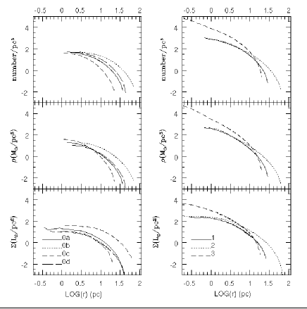
Figure 1: Initial number density (top panels), mass density (middle panels), and surface density (bottom panels) for each of the initial models.

Figure 2: Cumulative distribution of stars for each mass group in the labelled models. The highest/lowest curves correspond to the largest/smallest mass group (i.e. bin number $\alpha$ increasing upwards). The mass range encompassed by a curve representing mass bin $\alpha$ can be found by multiplying the mass of the model (column 2 of Table 1) by the mass fraction $dm_{\alpha}$ in bin $\alpha$ for the appropriate mass function index $x$ (see Table 2).

Table 1: Description of Models.

Model	mass	$r_{\rm half}$	$N$	$W_{0}$	# density	$x$	$T_{\rm dyn}$	$T_{\rm relax}$	orbits
	$10^{5}M_{\odot}$	pc			#$/pc^{3}$		$10^{6}$ years	$10^{9}$ years
0a	0.34284	10.6	142365	4	50	1.35	6.19	2.68	p1-3,d1-2
0b	2.73969	21.2	1136640	4	50	1.35	6.19	17.66	p1
0c	0.20614	6.24	29904	4	50	0.00	3.61	0.383	p1
0d	0.43807	13.4	269366	4	50	2.50	7.74	6.00	p1
1	1.22626	7.36	508669	6	1000	1.35	1.89	2.62	p1,p2,d1
2	2.86636	14.1	1186585	9	1000	1.35	3.28	9.92	p1
3	3.30330	4.62	1368230	12	1.0 $\times 10^{5}$	1.35	0.573	1.98	p1,p2

Columns: (1) Model number; (2) mass; (3) half mass radius; (4) number of stars; (5) King model; (6) central number density; (7) mass function index; (8) internal dynamical time (see equation [9]); (9) half-mass relaxation time; (10) orbits simulated.

Four representative cluster models (labelled 0-3) are considered, with properties summarised in Table 1. Model 0a was repeated with the same number density profile, but larger mass (Model 0b), and with different mass function indices (Models 0c and 0d). Figure 1 shows the number density and mass density as a function of spherical radius, and surface brightness as a function of projected radius for each initial distribution. Masses are converted to visual magnitudes and luminosities in this and subsequent plots using Bergbusch & VandenBerg’s (1992) isochrone for a 14 Gyr, [Fe/H]=-1.66 cluster. Figure 2 illustrates the level of mass-segregation by showing the cumulative fraction of stars within a given radius for each mass group in the models.

The cluster is generated as a Monte Carlo realisation of the Michie–King distribution function, using 8 discrete mass groups and a truncated, evolved power law initial mass function as described in Sigurdsson & Phinney (1995). The structure of each cluster is determined from a set of input parameters: the depth of the central potential, $W_{0}$, the central number density, $n_{0}$, and the mean central dispersion, $\sigma$. Some of the observable structure parameters, such as the concentration, core radius and light profile, are derived quantities and depend on the mass function and mass–luminosity relation chosen.

The particles representing the stars in mass group $\alpha(=1\ldots 8)$, of mass $m_{\alpha}$, are assumed to have some initial distribution function, $g_{\alpha}(\varepsilon)$, where $\varepsilon=-\Phi-{1\over 2}{\bf v}^{2}$ is the energy and ${\bf v}$ is the velocity of the particle (both in the cluster centre–of–mass frame), and $\Phi$ is the cluster potential. The distribution function is then given by

$$g_{\alpha}(\varepsilon)={{n_{0_{\alpha}}}\over{(2\pi\sigma_{\alpha})^{3/2}}}\Bigl{[}e^{{{\varepsilon}/{\sigma_{\alpha}}}}-1\Bigr{]},$$ (3)

where $\sigma_{\alpha}$ is the core dispersion of mass group $\alpha$ and the $n_{0_{\alpha}}$ are the normalised densities of each mass group. The $n_{0_{\alpha}}$ are solved iteratively given the cluster structure parameters, according to the scheme described in Sigurdsson & Phinney (1995).

Table 2: Adopted Mass Functions with Index $x$

$\alpha$		$x=0.0$			$x=1.35$			$x=2.50$
	$m_{\alpha}$	$dm_{\alpha}$	$f_{\alpha}$	$m_{\alpha}$	$dm_{\alpha}$	$f_{\alpha}$	$m_{\alpha}$	$dm_{\alpha}$	$f_{\alpha}$
1	0.12629	0.01847	1.00000	0.12346	0.23393	1.00000	0.12114	0.50252	1.00000
2	0.22461	0.04963	1.00000	0.21330	0.29045	1.00000	0.20449	0.33330	1.00000
3	0.34806	0.02601	1.00000	0.34600	0.08360	1.00000	0.34427	0.05484	1.00000
4	0.44265	0.03596	1.00000	0.43956	0.08355	1.00000	0.43695	0.04163	1.00000
5	0.57392	0.12309	0.34155	0.56679	0.13430	0.52623	0.56126	0.03946	0.67655
6	0.71009	0.16844	0.32948	0.70416	0.11552	0.58798	0.70078	0.02525	0.77595
7	0.99995	0.22745	0.00000	0.96585	0.04281	0.00000	0.93946	0.00264	0.00000
8	1.38462	0.35095	0.00000	1.36336	0.01583	0.00000	1.34231	0.00036	0.00000

Columns: (1) – mass group; (2), (5) and (8) – average mass $m_{\alpha}$; (3), (6) and (9) – mass fraction $dm_{\alpha}$; (4), (7) and (10) – fraction of luminous stars assigned to bin $\alpha$.

For each mass function index $x$ considered in this paper, Table 2 gives the average mass $m_{\alpha}$ of stars and total mass fraction $dm_{\alpha}$ assigned to bin $\alpha$, along with the fraction $f_{\rm\alpha}$ of stars in each bin that are luminous. Stars that have evolved beyond the main–sequence turnoff are assigned to remnant stellar classes. In particular, stars with initial masses between the turnoff and $4.7M_{\odot}$ are assumed to have evolved to white dwarfs, and stars with initial masses between $8$ and $15M_{\odot}$ are assumed to have formed $1.4M_{\odot}$ neutron stars. This follows the prescription in Chernoff & Weinberg (1990). Future work will consider other prescriptions for assigning remnant masses as a function of initial stellar mass. The presence of a substantial population of intermediate mass white dwarfs changes the present day mass function from the simple power law of the initial mass function. In particular, there is a pronounced ‘bump’, an excess of stars with masses $\sim 0.5M_{\odot}$ in the distribution function, which complicates interpretation of the local luminosity function in terms of the mass function, for intermediate mass stars.

Each cluster is generated by a simple acceptance–rejection algorithm, selecting particle masses, positions and velocities from the distribution function. The masses are assigned in discrete mass bins, with the value of the mass in each bin being the mean mass of that interval, weighted by the evolved mass function. That is, the mean mass in each bin allows for the presence of stellar remnants in that bin. Future models may incorporate a continuous distribution of stellar masses. The positions are drawn from a radial grid (typically of about 200 points, spaced to sample the density profile efficiently). A particle selected to be at radius $r_{i}$ is assigned to some radius $r_{i}\pm\epsilon$ where $\epsilon$ is a uniform random variable on the grid space interval. The initial distribution is thus a set of thin stepped radial shells, with local density that deviates slightly from the true density profile. Phase mixing ensures that the model settles down to a smooth representation of the cluster on a dynamical timescale. The initial model has a virial ratio $\sim 1\pm 1/\sqrt{N}$, and is stationary and stable. Cluster models were run in isolation using the SCF code (see §2.4.1 and Hernquist & Ostriker 1992): the initial mass segregation is robust and there is no spurious evolution. The mass segregation corresponds to thermal equilibrium for the cluster structure parameters (central potential and initial mass function) chosen. This is the equilibrium state expected for the internal distribution of masses within the cluster once the time scale for mass loss due to stellar evolution becomes longer than the core relaxation time, and provided that tidal effects have not yet had a strong effect on the cluster. There is also some evidence for primordial mass segregation in young clusters [Fischer et al. 1998, Elson et al. 1998], possibly due to bias in the formation of massive stars towards high density regions, or due to rapid relaxation in the young cluster. Mass segregation continues on a relaxation time scale, and would lead to core collapse in the absence of other effects.

2.3 Cluster orbits in the Galactic potential

A three-component model is used to represent the Galactic potential: $\Psi=\Psi_{\rm disk}+\Psi_{\rm spher}+\Psi_{\rm halo}$, in which the disk is represented by a Miyamoto-Nagai potential [Miyamoto & Nagai 1975], the spheroid by a Hernquist potential [Hernquist 1990], and the halo by a logarithmic potential:

$$\Psi_{disk}=-{GM_{\rm disk}\over\sqrt{R^{2}+(a+\sqrt{z^{2}+b^{2}})^{2}}},$$ (4)

$$\Psi_{\rm spher}=-{GM_{\rm spher}\over r+c},$$ (5)

$$\Psi_{\rm halo}=v_{\rm halo}^{2}\ln(r^{2}+d^{2}).$$ (6)

Here, $M_{\rm disk}=1.0\times 10^{11},M_{\rm spher}=3.4\times 10^{10},v_{\rm halo}=128,a=6.5,b=0.26,c=0.7$, and $d=12.0$, where masses are in $M_{\odot}$, velocities are in km s^-1 and lengths are in kpc. This choice of parameters provides a nearly flat rotation curve between 1 and 30 kpc and a disk scale height of $0.2$ kpc. The radial dependence of the z epicyclic frequency ($\kappa_{z}$) in the disk between radii at 3 and 20 kpc is similar to that of an exponential disk with a 4 kpc scale length.

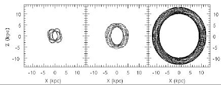
Figure 3: Locus of polar orbits p1 (left hand panel), p2 (middle panel) and p3 (right hand panel). The Galactic plane is at $Z=0$.

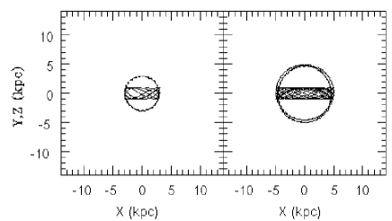
Figure 4: Locus of disk orbits d1 (left hand panel) and d2 (right hand panel). The solid line is for motion perpendicular to the Galactic plane (i.e. $Z-X$ motion) and the dotted line is for motion in the Galactic plane (i.e. $Y-X$ motion).

Table 3: Description of Orbits.

Orbit	$r_{\rm peri}$	$r_{\rm apo}$	$T_{\rm orb}$	$A_{\rm disk}$	$T_{\rm disk}$	$A_{\rm bulge}$	$T_{\rm bulge}$
	kpc	kpc	$10^{7}years$	(km s-1)/kpc/Myear	$10^{6}years$	(km s-1)/kpc/Myear	$10^{6}years$
p1	1.1	3.5	8.0	30	1.0	20-30	3.
p2	3.0	5.8	14.5	20	1.0	2-3	10.
p3	9.5	12.5	32.0	5-10	1.0	0.5	20.
d1	2.9	3.15	8.5	30	2.0	3-4	12.
d2	4.6	5.4	14.5	30	2.2	1	20.

Columns: (1) orbit; (2) closest approach; (3) apocentre; (4) azimuthal orbital time period; (5) defined in equation (14); (6) timescale for disk passage (see equation [8]); (7) and (8) as columns (5) and (6) but for bulge passages.

To contrast the evolution of the models in different tidal fields we choose orbits roughly 3kpc, 5kpc and 10kpc from the Galactic centre, three with polar orientations (p1, p2 and p3) and two near the Galactic disk (d1 and d2). Figures 3 and 4 show the paths of these orbits and Table 3 gives their peri- and apo-galacticon and radial time periods.

Hereafter we refer to the simulation representing the evolution of cluster Model $m$ along orbit $o$ as Model $(m,o)$.

2.4 Integration methods

Individual particle trajectories are integrated using a leapfrog integration scheme, with accelerations calculated from

$${\bf\ddot{r}}=\nabla(\Psi({\bf r})+\Phi({\bf r}))+{\bf a_{dyf}}+{\bf a_{kick}},$$ (7)

where the Milky Way is represented by the rigid potential $\Psi$ given in §2.2, and the cluster’s internal potential $\Phi$ is calculated from the particles’ masses and positions using the SCF code described in §2.4.1. The effect of accelerations due to two-body effects (i.e. terms ${\bf a_{dyf}}+{\bf a_{kick}}$) were included in only one simulation using the method described in §2.4.2. Dynamical friction of the cluster’s orbit was ignored. In all cases, the time step was smoothly varied along the orbit between $T_{\rm disk}/100$ and $T_{\rm dyn}/100$ to ensure that energy was conserved to better than 1 percent of the initial internal potential energy of the cluster. Here

$$T_{\rm disk}=b/v_{z}$$ (8)

is the timescale for a disk passage, where $b$ is the vertical scale of the Galactic disk (see equation [4]), and $v_{z}$ is the z-component of the satellite’s velocity as it crosses the disk plane at $Z=0$, and

$$T_{\rm dyn}=\pi\sqrt{r_{\rm half}^{3}\over 2Gm_{\rm sat}},$$ (9)

is the internal dynamical timescale for a system of total mass $m_{\rm sat}$ and half-mass radius $r_{\rm half}$ [Binney & Tremaine 1987]. The timescales for the orbits and models are given in Tables 3 and 1 respectively.

2.4.1 Self-consistent field code

The SCF code uses a bi-orthogonal basis function expansion to calculate the internal potential of the cluster from the individual particle positions and masses [Hernquist & Ostriker 1992]. The expansion is sensitive to large-scale fluctuations in the cluster’s potential but smooths local potential fluctuations arising from the discrete particles. Hence the SCF approach will underestimate relaxation when (as in our case) the number of particles in the simulation is equivalent to the number of stars in the system represented. The computations using this scheme (i.e. not including two-body encounters) were performed at the National Center for Supercomputing Applications (NCSA) with a version of the SCF code which had been parallelised to run on the Connection Machine 5 [Hernquist et al. 1995]. On average, each step required $4\times 10^{-4}$cpusec/particle/processor.

2.4.2 Two-body relaxation calculation

In order to explore the consequences of continuing mass segregation and two–body relaxation on the structure of the cluster, we incorporated a Fokker–Planck diffusion scheme into a version of the SCF code parallelised to run on the T3E [Sigurdsson et al. 1997] at the Pittsburgh Supercomputing Center. The results of Model (0a,p3), run with and without diffusion are compared in in §3.3.

The Fokker–Planck scheme calculates the first and second order velocity diffusion coefficients, $D(\Delta v_{i}),D(\Delta v_{i}\Delta v_{j})$ [Binney & Tremaine 1987]. The diffusion is directly incorporated into the explicit time evolution of the particles by including the last two terms in equation (7), where ${\bf a_{dyf}}$ is the dynamical friction experienced by the star, and ${\bf a_{kick}}$ is the effective acceleration due to scattering by individual stars in the cluster (see Sigurdsson & Phinney 1995 for discussion).

To calculate ${\bf a_{dyf}}$ and ${\bf a_{kick}}$, we choose an orthonormal basis local to each particle defined by the particle’s velocity ${\bf v}$ and position ${\bf x}$ in the cluster frame. This gives us three independent diffusion coefficients, $D(\Delta v_{\parallel})$, $D(\Delta v^{2}_{\parallel})$, and $D(\Delta v^{2}_{\perp})$. To calculate those we need the local density, which is obtained directly from the SCF expansion [Hernquist & Ostriker 1992], and a local velocity distribution. We approximate the velocity distribution as a Gaussian, and calculate it every $N_{v}\sim 100$ integration steps, by sampling the velocity distribution in radial bins, calculating the local dispersion, and using spline interpolation to obtain the dispersion as a function of radius. Provided the dynamical evolution of the cluster is slow compared to the dynamical time scale, the sparse updating of the dispersion profile is adequate, and provided the cluster is close to being relaxed, the approximation of taking the velocity distribution as an isotropic Gaussian is acceptable. The diffusion approximation incorporates a Coulomb logarithm term whose magnitude is uncertain to a magnitude comparable to other errors incurred by the approximations we make. Near the truncation radius, the interpolation of the dispersion must be positive definite or negative dispersion may be inferred. Outside the truncation radius the diffusion coefficients may be set to zero, or the local dispersion approximated by the Keplerian velocity due to the total enclosed mass.

Given the diffusion coefficients, then ${\bf a_{dyf}}=D(\Delta v_{\parallel})$ and we model ${\bf a_{kick}}$ by random fluctuations in velocity, $\Delta{\bf v}$, where ${\bf a_{kick}}={{\Delta{\bf v}}\over{\Delta t}}$, with

$$\Delta v^{2}_{\parallel} =\varsigma_{i}^{2}(D(\Delta v^{2}_{\parallel})\Delta t)$$ (10)

$$\Delta v^{2}_{\perp} =\varsigma_{i}^{2}(D(\Delta v^{2}_{\perp})\Delta t),$$ (11)

where $\varsigma_{i}$ is a random number with zero mean and unit standard deviation, chosen here from a normal distribution.

This choice of diffusion coefficients provides a fast and surprisingly good approximation to two–body relaxation in clusters, and allows a fair representation of the effects of two–body relaxation on the structure of the cluster in the presence of other perturbing dynamical processes. For isolated clusters, this scheme provides a realisation of evolution towards core collapse on relaxation time scales, and can follow the evolution of the cluster over several orders of magnitude in central density. Ultimately though, with a finite number of expansion terms, the SCF code fails to resolve the resulting density cusp and core collapse to infinite density is not observed. Details of the scheme will be discussed in another paper.

2.5 Analysis methods

2.5.1 Isolating the bound population of the cluster

In parts of this study, identical analyses are performed on the particle data from the simulations both with and without the unbound particles, and the results are compared. Much of the discussion of the interpretation of observations rests upon the identification of stars that are cluster members. We define members of the cluster to be the maximum set of mutually bound particles. This set is found iteratively, starting from the set of all particles, by: (i) calculating the internal potential field of the particles in the set considered; (ii) finding the velocity of each particle with respect to the velocity of the minimum of this potential field; (iii) defining each particle’s internal kinetic energy to be the kinetic energy of this relative motion; (iv) labeling those particles whose internal kinetic energy is greater than their internal potential energy as ‘unbound’, removing them from the set considered and returning to step (i). Steps (i)-(iv) are repeated until no new particles in an iteration are labelled ‘unbound’. Using this method we find that the instantaneous mass bound to the cluster is a monotonically decreasing function of time, and the number of stars that later become bound again to the cluster once they have first been classified as unbound is negligible.

2.5.2 Extrapolating mass functions

Each particle in our simulations is assigned the average mass $m_{\alpha}$ of the mass bin $\alpha$ that it occupies. The first four mass bins contain only luminous matter, the next two contain a fraction $f_{\alpha}$ of luminous stars and the two most massive bins contain only stellar remnants (see Table 2). Hence, we can trivially find the mass function of observable stars in any sample at these average points by calculating

$$\left({dN\over dm}\right)_{\alpha}={f_{\alpha}N_{\alpha}\over\Delta m_{\alpha}},$$ (12)

where $\Delta m_{\alpha}$ is the width of the mass bin and $N_{\alpha}$ is the number of stars in the bin. Since mass functions are typically calculated from stars near the turnoff in a globular cluster, we estimate $x$ using only the two heaviest luminous mass bins to be

$$x={LOG(N_{6}f_{6}\Delta m_{5})-LOG(N_{5}f_{5}\Delta m_{6})\over LOG(m_{6})-LOG(m_{5})}-1.$$ (13)

3 GENERAL EVOLUTION IN A TIDAL FIELD

3.1 Cluster heating

We expect mass loss to occur predominantly where the tidal field of the Milky Way is strongest – i.e. at pericentric points along the orbit and during disk passages. In column 5 of Table 3 we give values for

$$A_{\rm disk}=d^{2}\Phi_{\rm disk}/dz^{2}.$$ (14)

For a globular cluster whose physical scale is given by its half mass radius $r_{\rm half}$, this can be used to estimate the specific energy change due to the disk passage in the impulsive regime,

$$\Delta E_{\rm imp}={1\over 2}\left(A_{\rm disk}T_{\rm disk}r_{\rm half}\right)^{2},$$ (15)

[Spitzer 1958] which we shall subsequently refer to as the shock strength, where $T_{\rm disk}$ is the timescale for the disk passage (see equation [8]). We expect this estimate to be appropriate when $T_{\rm dyn}\gg T_{\rm disk}$, and can otherwise use it as an upper limit on the average energy change. Columns 7 and 8 in Table 3 give similar estimates for the importance of bulge shocking for these orbits (with $A_{\rm bulge}=d^{2}\Phi_{\rm bulge}/dR^{2}$), which is clearly competitive with disk shocking for orbit p1 (see Aguilar, Hut & Ostriker 1988 for a discussion of this effect). In our chosen Galactic potential, all these orbits lie within the core radius $d=12$kpc of the halo component (see equation [6]), so its tidal field is roughly constant along the orbit and halo shocking is unimportant (in contrast, this is likely to be an important factor in the evolution of the Sagittarius dwarf spheroidal galaxy – see Johnston, Spergel & Hernquist 1995).

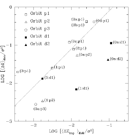
Figure 5: Average potential change per disk shock for each model as a function of shock strength, in units of the clusters’ internal velocity dispersion $\sigma$. Each point is labelled with the model and orbit. The dotted line indicates the trend expected when the impulse approximation is valid.

To test the accuracy of the impulse approximation, we calculated the change in the cluster’s internal potential energy per unit mass ($\Delta\Phi$) and the impulsive estimate for this change ($\Delta E_{\rm imp}$ – from equations [8], [14] and [15]) for each of the $N_{\rm disk}$ disk passages in each simulation. The points in Figure 5 show the average values of these quantities in the simulations, in units of the cluster’s velocity dispersion, $\sigma^{2}$. The models in the bottom left hand corner of the plot are expected to be the most resilient to the Milky Way’s influence.

There is a large spread in the response of the clusters’ potential energy for a given shock strength, $\Delta E_{\rm imp}$. The clusters on disk orbits (filled symbols) are shocked less noticeably than those on polar orbits (open symbols), because the timescales for the disk passages in the former case are longer, and the impulse approximation will only be valid in the outer region of the cluster. In general, Figure 5 shows that while this crude estimate serves as a useful guide to the importance of shock heating for a cluster in a given orbit a much more detailed calculation of the interaction of the internal and external dynamics is needed for an accurate assessment of cluster evolution in general. More rigorous analytic estimates for tidal heating have been discussed extensively elsewhere in the literature [Weinberg 1994, Kundic & Ostriker 1995, Gnedin & Ostriker 1997, Johnston et al. 1998].

3.2 Differential mass loss

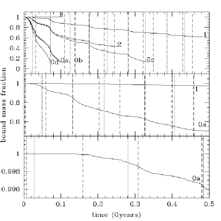
Figure 6: Bound mass fraction as a function of time for the models along the polar orbits p1 (top panel), p2 (middle panel) and p3 (lower panel). The dashed lines label the time of disk passages and the dotted lines label the time of pericentric passages.

Figure 7: Bound mass fraction as a function of time for the models along the disk orbits d1 (top panel) and d2 (bottom panel). The dashed lines label the time of disk passages.

Figures 6 and 7 follow the bound mass fraction remaining as a function of time for the first 0.5 Gyrs of evolution along the polar and disk orbits. On each of these figures we show the time of disk passages as vertical dashed lines, and the pericentric points along the orbits as vertical dotted lines. As noted in the previous section, the mass loss rate is greatest at these locations along the orbit. A comparison of these plots with Figure 5 confirms the loose correlation between mass loss rate and shock strength.

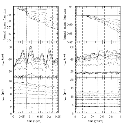
Figure 8: Bound mass fraction, limiting and half mass radii for each mass group as a function of time for Model (1,p1) (left hand panels) and Model (0a,p3). The vertical dashed and dotted lines give the time of disk and pericentric passages respectively. The outer solid lines in each panel are for the least and most massive stars and the dotted lines are for the intermediate mass stars.

Figure 8 compares the effect of the tidal field on each individual mass group in Model (1,p1) (left hand panels) with those in Model (0a,p3) (right hand panels). The solid lines are for the smallest and largest masses and the dotted lines are for the intermediate ones. The top panels illustrate differential mass loss due to mass segregation, as the most weakly bound (and therefore lower mass) stars are preferentially stripped. The lower two panels give a measure of the response in the spatial distributions - $r_{\rm lim}$ is calculated as the average radius of the outermost 1 percent of bound particles in each group, and $r_{\rm half}$ is calculated as the radius containing half the mass of each group. Again, the compressive disk shocks (and subsequent expansion due to the energy input) are clearly seen. The effect is more dramatic in the left hand panels since this model is more susceptible to the influence of tides (as demonstrated by its position in Figure 5, and large mass loss rate). Similar characteristics are seen in all the models.

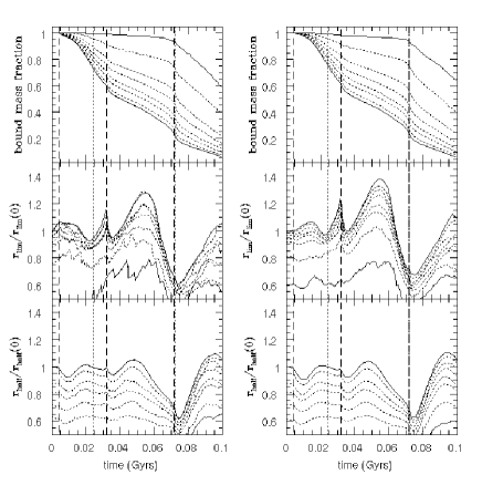
Figure 9: As Figure 8 but for Models (0a,p1) and (0b,p1).

Figure 9 repeats Figure 8 for Models (0a,p1) (left hand panels) and (0b,p1) (right hand panels). These models had identical mass density profiles, but with different radial scales (and hence total masses). The comparison of the two demonstrates that the general characteristics of the response for models with the same density profiles subjected to the same tidal field are identical.

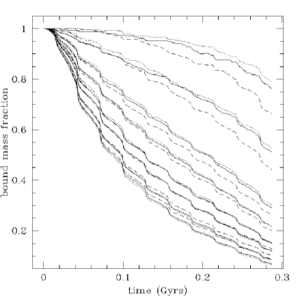
Figure 10: The solid lines show the evolution of the bound mass fraction for each mass group in Model (0a,d1). The dashed lines show the fraction of each mass group within a spherical surface in the initial model which contains the same total mass as is instantaneously bound to the satellite. The dotted lines show the fraction of each mass group within an energy surface in each initial model which contains the same total mass as is instantaneously bound to the satellite.

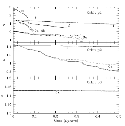
Figure 11: The solid lines show the evolution of the mass function index $x$ along each of the polar orbits. The dashed lines give $x$ for the mass within a spherical surface in each initial model equivalent to the bound mass remaining in the simulations at that time. The dotted lines show $x$ within an equivalent energy surface in each initial model.

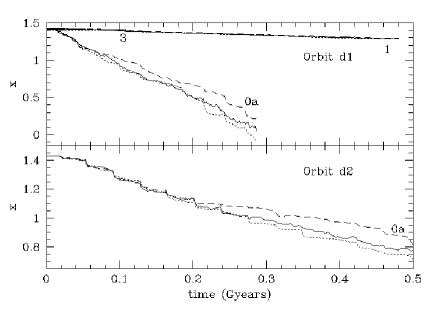
Figure 12: As Figure 11 but for the disk orbits.

Figures 10 – 12 illustrate our intuitive understanding of tidal mass loss in a mass-segregated system. As an example, the solid lines in Figure 10 show the bound mass fraction for each mass group as a function of time for Model (0a,d1). The dashed lines show the prediction if the initial model were simply truncated in radius at the surface enclosing the same mass as is instantaneously bound to the system in the simulation. The dotted lines show the prediction if the initial model is instead truncated in binding energy. As might be anticipated, initial binding energy provides the more accurate of these simple guides to which stars are lost first from the system. This behaviour is seen in all our simulations, as shown in Figures 11 and 12. The solid lines show the global mass function index $x$ as a function of time for each simulation, the dashed lines show the result of estimating $x$ by truncating the initial model in radius and the dotted lines show $x$ for truncation in energy. Note in general that the agreement is good, except when there has been substantial evolution of the system (e.g Models (0a,p1), (0c,p1)).

In summary, the results in this section demonstrate that: (i) the impulse approximation provides a rough guide to the mass loss rate from a system; (ii) tidal mass loss along a given orbit is determined by the density profile of the cluster; and (iii) tidal shocking of a mass-segregated system leads to evolution of the mass function, which can approximately be predicted for a given mass lost by simply truncating the initial distribution in energy. Clearly these general trends fit in with theoretical interpretations of observed correlations of cluster properties with $R_{\rm GC}$ and $Z$ [Capaccioli et al. 1991, Capaccioli, Piotto & Stiavelli 1993, Djorgovski, Piotto & Capaccioli 1993]. However, a quantitative comparison of our simulations with observations would require more detailed analytic models both of the tidal effects seen in the simulations and of other physical processes not included (one example is given in the next section) and is beyond the scope of the current study.

3.3 Competition of tides and relaxation

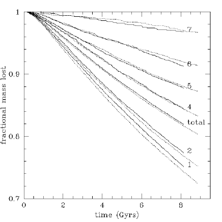
Figure 13: Bound mass fraction as a function of time for the labelled mass groups in Model (0a,p3) run with (dotted lines) and without (solid lines) diffusion.

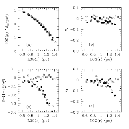
Figure 14: Comparison of initial (stars) and final properties of Model (0a,p3) run with (open squares) and without (closed squares) diffusion.

Figure 13 compares the mass loss rate for each group in Model (0a,p3) evolving over 8 Gyrs both with (dotted lines) and without (solid lines) diffusion included. The half-mass relaxation time for this cluster is $T_{relax}\sim 2.68$ Gyrs (see Table 1). The evaporation time for a cluster is $\sim$ 100 $T_{\rm relax}$ [Meylan & Heggie 1997], so we expect only a few percent change in bound mass fraction due to relaxation over the course of the simulation, as is seen in the figure. Relaxation contributes to mass loss by increasing the number of low mass stars lost and decreasing the number of high mass stars lost, with a net increase in mass loss. Hence, the evolution of the mass function will be modified from the purely tidal response described in the previous section. Figure 14 shows that the density and velocity properties of the model evolved with (solid squares) and without relaxation (open squares) are similar (the initial model is shown in stars).

These figures demonstrate that our neglect of relaxation in the models considered in this paper will not substantially affect their evolution since a significant fraction of mass is lost due to tidal influences over a few relaxation times. In contrast, Pal 5 is an example of a cluster whose evolution is thought to be dominated by relaxation [Rosenberg et al. 1998] and a natural extension to our work would be to consider models where the tidal and evaporation mass loss rates are comparable [Vesperini & Heggie 1997].

4 INTERPRETING OBSERVATIONS OF TIDALLY DISRUPTING, MASS-SEGREGATED SYSTEMS

4.1 ‘Observing’ the simulations

Observed properties of globular clusters are often interpreted as resulting from the tidal influence of the Milky Way. In this section, we ‘observe’ our models to confirm the validity of some common interpretations and explore other signatures of tidal disruption that future studies might be sensitive to. We focus our analysis on Model (0a,p3) as an example of a cluster with a steady mass loss rate that could survive for the lifetime of the Galaxy. We examine the observable properties of this model at the end of the simulation (after 8 Gyrs of evolution), and compare and contrast it with the same model at earlier times and with the other models in our sample.

Since the Sun’s position along the Solar Circle in the simulations is arbitrary, rather than assuming a single viewpoint we examine each set of particle data along three perpendicular axes defined by the cluster’s instantaneous position and velocity: the $x$ axis lies along the vector joining the cluster to the Galactic centre; the $z$ axis is perpendicular to the cluster’s position and velocity vector (i.e. looking down on the orbital plane); and the $y$ axis is perpendicular to these two, along the orbit of the satellite (i.e. it coincides with the velocity vector when the Galactocentric radial velocity is zero). We also make the simplification that the lines of sight across the face of the cluster are perfectly parallel (i.e. the observer is at infinite distance from the cluster) and state distances in our projected coordinates in $pc$ rather than $arcmin$. This will not significantly affect our analysis of density profiles in §4.2, but can alter the measurement of cluster rotation, and we discuss this simplification further in §4.3.

4.2 Star count profiles

4.2.1 Qualitative interpretation

Figure 15: Number count surface density profiles along labelled views (see §4.1) and down to various limiting magnitudes ($M_{\rm to}$ is the magnitude of the turnoff) for the final bound population (filled squares) and all stars (open squares) for Model (0a,p3).

Figure 15 shows the number surface density for all stars (top panels), stars brighter than 4 magnitudes below the turnoff (middle panels) and stars down to the turnoff (bottom panels) at the end of the simulation of Model (0a,p3) with the three labelled viewpoints along the axes defined in §4.1. The closed symbols are for stars still bound to the satellite and the open symbols include unbound stars in the calculation (where the ‘bound’ and ‘unbound’ populations are separated following the method described in §2.5.1).

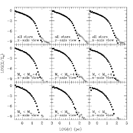
Figure 16: Number count surface density profiles along the $x$-axis for the bound population (filled squares) and all stars (open squares) at random points along the orbit for labelled models. The dashed lines show the surface density for extra-tidal material from equation (17) and the dotted lines show the adopted $r_{\rm break}$ in each case, for use in the mass loss estimates.

In this Figure, there is a clear break in the slope of the profile defined by the open symbols, approximately corresponding to the point where the closed and open symbols become distinct and the fraction of unbound stars in an annulus becomes significant. Such ‘extra-tidal’ stars have been detected in several studies of dwarf spheroidal galaxies [IH95, Kuhn et al. 1996] and globular clusters [G95, Grillmair 1998]. Our investigation confirms the common interpretation that these can be identified as stars escaping from the satellites. Figure 16 demonstrates that this is a general result by repeating the $x$-axis view for all stars in Model (0a,3p) at earlier times (left hand panels) and at random points for several of the other models (as labelled).

4.2.2 Quantitative interpretation

Tremaine (1993) pointed out that the change in the orbital frequency of a star torn from the satellite at radius $r_{\rm break}$ (the point at which the slope of the surface density profile changes) should approximately be given by $\Delta\Omega\sim r_{\rm break}d\Omega/dR$, where $\Omega(R)$ is the frequency of a circular orbit in the parent galaxy at radius $R$. Equivalently, the orbital energies in tidal debris from a satellite orbiting in a potential $\Phi$ will be spread over a characteristic range $\epsilon=r_{\rm tide}d\Phi/dR$. Johnston (1998) tested this simple physical argument by looking at the spread in energies in streamers seen in numerical simulations of tidal disruption and found that $\epsilon<|\Delta E|<2\epsilon$. Hence, debris will spread over an angular distance comparable to the size of the cluster ($r_{\rm break}/R$) in a time $(r_{\rm break}/R)/2\Delta\Omega\sim T_{orb}/\pi$, where $T_{\rm orb}$ is the azimuthal time period of the orbit. This suggests that we can estimate the average surface density of stars in an annulus between $r_{\rm break}$ and $r$ from the centre of the cluster to be

$$\langle\Sigma_{\rm xt}(r)\rangle={1\over g(\theta)}\left[{dm\over dt}{(r-r_{\rm break})\over r_{\rm break}}{T_{\rm orb}\over\pi}\right]$$ (16)

$$\left/\left[\pi(r^{2}-r_{\rm break}^{2})\right]\right.,$$

where $dm/dt$ is the mass loss rate from the cluster. The function $g$ depends on the angle $\theta$ of our line of sight with the plane perpendicular to the direction of motion of the satellite. Eventually, the debris spreads out along the satellite’s orbit so we can take $g(\theta)=\cos\theta$ as a crude approximation. In fact, mass tends to leave the satellite at the inner and outer Lagrange points along the vector joining the satellite to the centre of the galaxy, so the geometry of the streamers close to the satellite is rather more complicated than this.

We can differentiate equation (16) to find an approximate expression for the absolute surface density

$$\Sigma_{\rm xt}(r)={1\over g(\theta)}{dm\over dt}{T_{\rm orb}\over\pi}{1\over 2\pi r_{\rm break}r}.$$ (17)

This estimate is overlaid in dashed lines on the profiles shown in Figure 16 using $dm/dt$ averaged over each simulation, $T_{\rm orb}$ from Table 3 and $r_{\rm break}$ indicated by the vertical dotted lines in each panel. The open squares and dashed line agree well in all cases except for Model (3,p1). In this model, the simulation was run for only a few orbital periods so the debris only had time to disperse a few $r_{\rm break}$ from the satellite and the streamers were not well populated.

Equation (17) and Figure 16 demonstrate that we expect the extra-tidal population around a cluster to have $\Sigma_{\rm xt}(r)\propto r^{-1}$. In observations of real globulars, the surface density of extra-tidal stars has been found to fall as $\Sigma_{\rm xt}(r)\sim r^{-\gamma}$ with $-5<\gamma<-0.7$ (G95; Zaggia, Piotto & Capaccioli 1997). This suggests that the measured $\gamma$ might be used as a test of whether the globular is sufficiently obscured, either by tidal debris further along its own tidal tail or by the Galactic field, that the above interpretation is invalid.

Note that these estimates are independent of the method of mass loss from the cluster since the dynamics once the star is lost is determined only by the external field, and hence should apply equally to mass lost by tidal stripping, shocking, or evaporation due to relaxation.

4.2.3 Estimating mass loss rates using extra-tidal stars

Equations (16) and (17) suggest two ways of estimating the fractional mass loss rate $(df/dt)$ from a cluster using observations of extra-tidal stars.

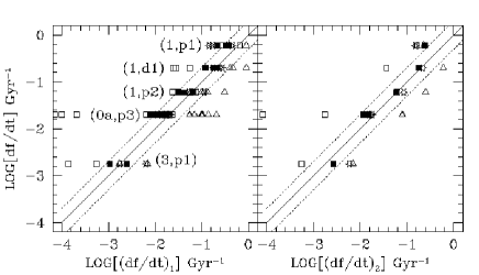
Figure 17: Known mass loss rate $df/dt$ (from Figures 6 and 7) for the labelled models plotted against the estimates $(df/dt)_{1}$ (left hand panel) and $(df/dt)_{2}$ (right hand panel). The solid squares, open squares and stars show the results when viewed from along the $x$, $y$ and $z$-axis respectively. The open triangles repeat the $y$-axis view but with $g(\theta)\equiv 1$. The solid line shows where the estimated and known mass loss rates agree, and the dotted lines are for factor of 2 discrepancies.

If the extra-tidal population is well defined out to a radius $r_{\rm xt}$ with $\Sigma_{\rm xt}\sim r^{-1}$ we can count the number of stars $n_{\rm break}$ within $r_{\rm break}$ (the point where there is a break in the slope of the surface density profile) and the number of extra-tidal stars $n_{\rm xt}$ between $r_{\rm break}$ and $r_{\rm xt}$ and use them to find

$$\left({df\over dt}\right)_{1}=g(\theta){r_{\rm break}\over r_{\rm xt}-r_{\rm break}}{n_{\rm xt}\over n_{\rm break}}{\pi\over T_{\rm orb}}.$$ (18)

Since the timescale for stars to diffuse beyond a few $r_{\rm break}$ is an orbital timescale, so long as $r_{\rm xt}>2r_{\rm break}$ this estimate should be sensitive to the average mass loss rate rather than the instantaneous one. The left hand panel of Figure 17 plots the known fractional mass loss rate, $df/dt$, for each of the models with fractional mass loss rates less than 1Gyr^-1 (see Figures 6 and 7) against $(df/dt)_{1}$ calculated from equation (18). To find $(df/dt)_{1}$, we evaluated the ratio $n_{\rm xt}/n_{\rm break}$ for $r_{\rm xt}=2r_{\rm break}$, $r_{\rm xt}=5r_{\rm break}$ and $r_{\rm xt}=10r_{\rm break}$. This process was repeated looking along the $x$-axis (solid squares), $y$-axis (open squares) and $z$-axis (stars). The open triangles show the estimate made along $y$-axis if the viewing angle is not taken into account (i.e. $g(\theta)\equiv 1$). The solid line in the figure shows where the estimated and known mass loss rates agree, and the dotted lines are for factor of 2 discrepancies. The figure suggests that we can use this technique to estimate the mass loss rate from a Galactic satellite provided our viewpoint lies close to the plane perpendicular to the satellite’s velocity vector (equivalent to the $xz$-plane in our projection). Otherwise, we are likely to poorly estimate the rate of mass loss as the debris along the satellite’s orbit confuses the calculation.

If the extra-tidal population is either not well defined or non-existent we can estimate $(df/dt)_{2}$ as an upper limit for the mass loss rate from $\Sigma_{\rm xt}(r_{\rm break})$, where $r_{\rm break}$ is taken to be the point either where the slope of the profile changes or the last point where the surface density is separable from the background. Then, from equation (17),

$$\left({df\over dt}\right)_{2}=g(\theta){\Sigma_{\rm xt}(r_{\rm break})\over n_{\rm break}}{\pi\over T_{\rm orb}}2\pi r^{2}_{\rm break},$$ (19)

which is shown in the right hand panel of Figure 17. As with the first case, the view perpendicular to the velocity vector provides the best estimate.

4.3 Line of sight velocity distributions

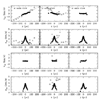
Figure 18: Line-of-sight velocity $v_{\rm los}$ and dispersion $\sigma_{\rm los}$ for bound (filled squares) and all stars (open squares) in Model (0a,p3). The line of sight for each column of panels is labelled in the top row (see §4.1 for axis definitions).

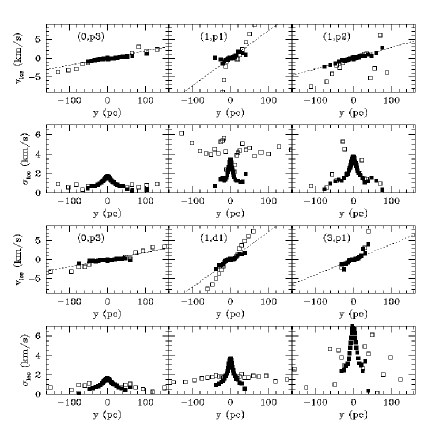
Figure 19: Repetition of panels $x$-axis view of Figure 18 for the labelled models at random points along the orbit.

Figure 18 summarises the line-of-sight velocity analysis at the end of the simulation for Model (0a,p3) from the stated viewpoints and with the observer assumed to be at infinite distance from the cluster (i.e with the individual lines of sight across the cluster assumed to be parallel to the one to the cluster centre – the effect of this simplification is discussed in §4.3.1). For each viewpoint the average $v_{\rm los}$ and dispersion $\sigma_{\rm los}$ in the velocities of stars are calculated in bins lying in strips along the two perpendicular axes across the cluster. Figure 19 demonstrates the general nature of these plots, repeating the $x$-axis view of Figure 18 at different orbital phases of this model and for several different models. The solid symbols show the analysis for the bound stars, and the open symbols shows the results for all stars.

4.3.1 Average velocities and cluster rotation

The average velocities are zero except for the viewpoints which are sensitive to the cluster’s orbital motion. In the panels corresponding to the $x$-axis view of Figures 18 and 19, the dotted lines indicate the expected velocity gradient if the cluster were rigidly co-rotating with its orbit. The bound stars follow this line fairly closely, with some indication of a smaller gradient in velocities towards the centres of the clusters. The unbound stars appear to be rotating faster than this as they move to orbits with higher/lower angular velocities to form the leading/trailing streamers.

In our analysis, two effects are clearly contributing to the measured rotation of the cluster – the intrinsic rotation of the cluster (in our simulations, roughly corresponding to co-rotation with the tidal field), and the velocity gradient in stripped material. Observers also have to contend with ‘perspective rotation’ [Feast, Thackeray & Wesselink, 1961, Merritt, Meylan & Mayor 1997, Drukier et al. 1997] from the projection of the tangential velocity onto the non-parallel lines of sight across the cluster. If we were indeed viewing a rigidly co-rotating cluster from the centre of the Galaxy, the intrinsic and perspective rotation would cancel each other out and we would be sensitive only to tidal stripping, but if we were closer to/farther from the cluster than the centre of the Galaxy, we would be dominated by the perspective/intrinsic rotation.

Unfortunately, we cannot assume that tidal torquing of a real satellite necessarily results in co-rotation. The rotation seen in our simulations is likely to be an artifact of the near-circular orbits we have chosen. In models, run along eccentric orbits, of the disruption of the Sagittarius dwarf galaxy, Johnston, Spergel & Hernquist (1995) found that the line of sight velocity gradient is dominated by perspective rotation, despite the fact that our viewpoint is farther from the satellite than the centre of the Galaxy, presumably because the satellite is not co-rotating. Velázquez & White (1995) made an estimate of 225km s^-1 for the tangential velocity of the Sagittarius dwarf galaxy by considering only the effect of perspective rotation and this roughly agrees with the observed proper motion of 250km s^-1 [Ibata et al. 1997].

Rotation has been detected in several observational surveys of Galactic globular clusters. Merritt, Meylan & Mayor (1997) analysed the phase-space distribution of 469 stars in $\omega$Cen and found, after taking perspective rotation into account, it to be consistent with solid body rotation out to 11pc from the centre of the cluster, and decreasing beyond. Drukier et al. (1997), in an analysis of the velocities of 230 stars in the outskirts of M15, found some evidence for rotation. In both these studies, rotation was found to be less important towards the edge of the cluster, suggesting that in these cases it is intrinsic and not due to tidal torquing or stripping of the bound system.

4.3.2 Velocity dispersions and tidal heating

In most panels of Figures 18 and 19 there is good agreement between $\sigma_{\rm los}$ calculated with and without the unbound stars. However, the observed results can be confusing when looking along the orbit ($y$-axis view panels of Figure 18), as there is significant unbound material along the line of sight from the trailing and leading streamers. This problem may not be so severe in reality if the sample can be selected to exclude stars beyond a few tidal radii from the cluster (in the figure, all stars at the projected separation were included).

An observer would also see an apparently enhanced velocity dispersion when looking at the outskirts of the cluster from the centre of the Galaxy. In particular, note that the dispersion in the unbound material roughly corresponds to the dispersion of the bound material within the point where stripping occurs. This suggests that satellites that are being more violently stripped will have larger dispersions in their debris trails, though not in excess of the maximum dispersion of the bound material. The Sagittarius dwarf spheroidal galaxy is an example of a system where it can be plausibly argued that this behaviour is observed: its highly distorted surface density contours suggest that it is likely to be surrounded by a cloud of unbound stars and its velocity dispersion is roughly constant along the entire length of its major axis [Ibata et al. 1997].

In their analysis of the velocities in the outskirts of M15, Drukier et al. (1997) found that the dispersion of the stars decreased to a minimum at 7 arcmin, increasing again beyond this radius. They suggest that this deviation from the behaviour expected for an isolated cluster could be due to tidal heating, and our simulations confirm this interpretation. They comment that the radial position of this minimum is much smaller than the tidal radius found by G95 by fitting King Models to star count profiles. This is also consistent with our analyses – the star counts and velocity analyses become contaminated by unbound stars well within the outermost radius of the bound system. Hence the minimum in the velocity dispersion profile is a good indicator of where this contamination becomes important, but does not necessarily correspond to the edge of the system.

4.4 Mass functions

4.4.1 Measuring present day mass functions

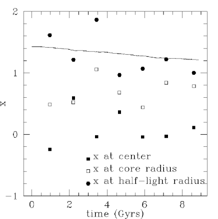
Figure 20: Mass function index $x$ as a function of time for all stars bound to Model (0a,p3) (solid line), and as measured at various points in the cluster.

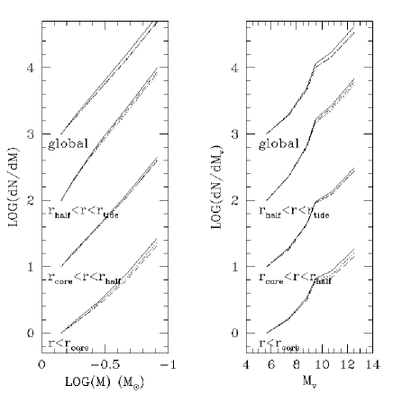
Figure 21: Initial (solid lines) and final mass and luminosity functions for Model (0a:p3) simulated with (dashed lines) and without (dotted lines) diffusion effects.

In Figures 20 and 21 we mimic the observational analyses recently applied to the globular clusters NGC 1261 [Zoccali et al. 1998] and M55 [Zaggia et al. 1997]. The solid line in Figure 20 shows the evolution of the mass function index $x$ for Model (0a,p3). The points indicate what $x$ would be measured to be at different points along the orbit and at different positions in the cluster if viewed from the centre of the Galaxy – within the core radius (filled squares), between the core and half-light radii (open squares) and between the half-light and tidal radii (stars). Each of these points is calculated using several thousand stars. In Figure 21 we plot the mass and luminosity functions at the beginning (solid lines), and the end (dotted lines) of the simulation. The dashed lines show the final analysis for the same Model but for the simulation that included relaxation effects.

4.4.2 Placing limits on the initial mass function of a cluster

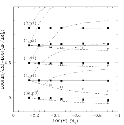
Figure 22: Global PDMF (dashed lines) and local PDMF (dotted lines) for outer 100 stars, for the labelled models. The mass functions have been normalized to the IMF of each model (represented by solid horizontal lines) and multiplied by arbitrary constants. The solid squares show the IMF reconstructed from the estimated mass loss rate, global and local mass functions. The open squares show the result of the same reconstruction, but using the outermost 1000 stars to find the local PDMF.

Suppose we have estimated the fractional mass-loss rate from a cluster using its observed population of extra-tidal stars. If we also know the PDMF, both globally and locally in the outskirts of the cluster, we can place some limits on its IMF. We test this idea with our simulations by using the methods outlined in §4.1 to find $(df/dt)_{1}$. Figure 22 shows the final mass function $(dN/dM)_{\rm final}$ at the end of the five labelled simulations (dashed line) and the mass function for the 100 stars at the projected edge of each system $(dN/dM)_{\rm edge}$ (dotted line), where each mass function has been scaled by the known IMF ($(dN/dM)_{0}$, represented by the horizontal solid line). We then simply estimate the IMF (solid squares) to be,

$$\left({dN\over dM}\right)_{0,\rm est}=\left({dN\over dM}\right)_{\rm final}+T_{\rm sim}\left({df\over dt}\right)_{1}\left({dN\over dM}\right)_{\rm edge}$$ (20)

where $T_{\rm sim}$ is the duration of the simulation. (The open squares show the result if the PDMF of the outermost 1000 stars is used.)

Several assumptions make this estimate uncertain: (i) $(df/dt)_{1}$ is taken from star counts, implicitly assuming that the mass function of the extra-tidal material is the same as the global mass function; (ii) we assume the mass-function of the stripped material to be constant with time; (iii) we neglect relaxation effects; and (iv) we assume that the satellite fills its tidal radius, and hence loses mass at a roughly constant rate due to either evaporation or tidal effects. The first approximation can be addressed if the luminosity function of the cluster is known as a function of radius, as is the case in our simulations – Figure 22 demonstrates that we can make reasonable predictions for the simulations even without this level of refinement; the second two assumptions will both lead to an underestimate of the evolution of IMF; and the last approximation will place some limits on how far back we might be able to ‘integrate’ the differential mass loss.

Despite these uncertainties, this method provides a new approach – more directly based on observations rather than using complex dynamical models – to exploring the question of whether the IMF in globulars was universal, or environment dependent.

5 DISCUSSION: APPLICATIONS TO OBSERVED SYSTEMS

5.1 Destruction rate of galactic satellites

5.1.1 Dwarf spheroidal galaxies

IH95 studied the morphology of eight of the dwarf spheroidal satellites of the Milky Way (all the ones currently known with the exception of Sagittarius) determined from star counts made using the APM facility at Cambridge. Extra-tidal stars are clearly seen in the number count profiles for six of these satellites, but in no case do they clearly follow $\Sigma_{\rm xt}\sim r^{-1}$. Hence, we use equation (19), to find an upper limit for the mass loss rate. Using the data from Table 3 of IH95 (kindly made available to us by M. Irwin), we subtract off the mean background stellar density from each of their bins and take $r_{\rm break}$ to be the smaller of the point at which the slope of the star count profile changes (by visual inspection of their figure 2) and the last measured surface density above the background. The orbital time period $T_{\rm orb}$ is calculated for a circular orbit in a logarithmic potential, with circular velocity $v_{c}=200$km s^-1

$$T_{\rm circ}={2\pi R_{\rm GC}\over v_{c}}=1.5\left({R_{\rm GC}\over 50{\rm kpc}}\right){\rm Gyrs},$$ (21)

with $R_{\rm GC}$ taken to be the current distance of each satellite from the Galactic centre. In fact, if the time period of orbits is assumed to be independent of angular momentum (shown to be approximately true in Johnston 1998), then a satellite at $R_{\rm GC}$ with velocity $v$ in the range $0<v<3v_{\rm c}/2$ will have an orbital time period $T_{\rm orb}$ in the range $T_{\rm circ}(R_{\rm GC})/2<T_{\rm orb}<2T_{\rm circ}(R_{\rm GC})$, so equation (21) is expected to be good to within a factor of 2. Several of the dwarf spheroidal satellites do have proper motion measurements – with large errors. These could in principle be used to determine a specific time period, but since the mass loss estimate itself is expected to be uncertain to within a factor of 2, the approximation in equation (21) is deemed to be sufficiently accurate. For those with proper motions we calculate the angle $\theta$ between our line of sight and the plane perpendicular to the velocity vector of the satellite in the Galactic rest frame. Otherwise, we assume the orbit is circular and calculate $\theta$ as the angle between our line of sight and the Galactocentric radius vector of the satellite.

Table 4: Mass loss rates for dwarf spheroidals.

Name	$R_{\rm GC}$	$T_{\rm orb}$	$\theta$	$(df/dt)_{2}$
	(kpc)	(Gyr)	(degrees)	(Gyr-1)
Carina	8.66E+01	2.60E+00	2.35E+01	$<$ 3.31E-01
Draco	7.20E+01	2.16E+00	4.50E+01	$<$ 2.18E-01
Fornax	1.22E+02	3.66E+00	2.94E+01	$<$ 6.17E-02
LeoI	2.02E+02	6.05E+00	5.61E+01	$<$ 5.92E-02
LeoII	2.10E+02	6.29E+00	3.66E+01	$<$ 1.44E-01
Sculptor	7.22E+01	2.16E+00	1.64E+01	$<$ 2.84E-01
Sextans	8.60E+01	2.58E+00	4.36E+01	$<$ 2.61E-01
Ursa Minor	6.59E+01	1.98E+00	1.30E+01	$<$ 3.22E-01

Columns: (1) name; (2) Galactocentric distance; (3) time period of circular orbit at that distance; (4) angle between line of sight and plane perpendicular to satellite’s velocity, calculated from proper motion measurements for Sculptor [Schweitzer, Cudworth, Majewski & Suntzeff (1995)] and Ursa Minor [Schweitzer, Cudworth & Majewski (1998)]; (5) mass loss rate estimate from equation (19).

All these quantities are shown in Table 4. The estimates $(df/dt)_{2}$ range from a few percent (Fornax and Leo I) up to more than 30 percent in the next Gyr (Ursa Minor and Carina). They do not correlate well with previous calculations that attempted to determine the robustness of each object either from the ratio of the expected to observed tidal radius (where the former was calculated given a dynamical estimate of the satellite’s mass), or of the external tidal field to internal field (see IH95). Nevertheless, these mass loss rates clearly indicate that the satellite system of the Milky Way could easily be diminished by several members in the next 10 Gyrs, which in turn suggests that there may have been several more satellites of the Milky Way in the past.

If these dSph do indeed have such large mass loss rates, why have we not detected tidal streamers? In the cases of Ursa Minor and Sculptor this question was addressed by Johnston (1998), using a semi-analytic technique. She found that if each was losing mass at the rate of 10 percent per Gyr the local number count densities along the streamers (i.e. not averaged over annuli centred in the cluster) would not exceed 1 percent of the background star counts predicted by the Bahcall-Soneira [Bahcall & Soneira 1980] model of the Milky Way. Hence, even increasing these mass loss rates to the tabulated values would not make the streamers striking features in the sky. However, the estimates bolster the notion that these streamers might be discovered and traced over large angular extents using integrated star counts (such as the method of Great Circle Cell Counts proposed by Johnston, Hernquist & Bolte 1996) or with color and velocity information to distinguish them from the background.

5.1.2 Globular clusters

Table 5: Mass loss rates for globular clusters.

NGC	$R_{\rm GC}$	$T_{\rm orb}$	$\theta$	$\gamma$	$(df/dt)_{1}$	$(df/dt)_{2}$	G&O
	(kpc)	(Gyr)	(degrees)		(Gyr-1)	(Gyr-1)	(Gyr-1)
288	1.14E+01	3.43E-01	4.19E+00	-5.21E-01	5.26E-02	1.26E-02	1.10E-01
362	9.04E+00	2.71E-01	1.40E+01	-1.58E-01	6.22E-01	5.77E-01	3.54E-02
1904	1.81E+01	5.44E-01	8.66E+01	–	–	$<$ 8.51E-03	3.54E-02
2808	1.07E+01	3.20E-01	2.33E+01	–	–	$<$ 4.37E-02	1.61E-02
3201	8.85E+00	2.65E-01	4.95E+01	–	–	$<$ 4.50E-01	3.45E-02
4590	9.94E+00	2.98E-01	5.17E-01	–	–	$<$ 1.28E+00	8.22E-03
5824	2.60E+01	7.81E-01	7.94E+01	-1.33E+00	6.46E-02	1.18E-01	3.06E-03
6864	1.17E+01	3.52E-01	8.60E+01	–	–	$<$ 4.91E-02	1.89E-02
6934	1.17E+01	3.52E-01	4.33E+01	–	–	$<$ 4.18E-01	2.89E-02
6981	1.22E+01	3.65E-01	5.84E+01	–	–	$<$ 2.96E-01	1.76E-02
7078	1.01E+01	3.02E-01	5.06E+01	–	–	$<$ 7.00E-02	2.17E-02
7089	1.01E+01	3.02E-01	1.91E+01	-1.62E+00	1.29E-01	3.13E-01	5.76-03

Columns: (1) name; (2) Galactocentric distance; (3) time period of circular orbit at that distance; (4) angle between line of sight and plane perpendicular to satellite’s velocity, calculated from proper motions in Dauphole et al. 1996; (5) slope of extra-tidal star surface density profile; (6) mass loss rate estimate from equation (18); (7) mass loss rate estimate from equation (19) (8) mass loss rate estimate from Gnedin & Ostriker (1997).

Table 5 presents the results of mass loss estimation for the 12 globular clusters analysed by G95 (using their tables 3-14, kindly made available to us by C. Grillmair). Four of these clusters have well-defined tidal tails with slopes $\gamma\approx 1$ (given in column 5), and in these cases both $(df/dt)_{1}$ and $(df/dt)_{2}$ are calculated. In the other cases, only the latter estimate is made as an upper limit on the mass loss rate. The estimated limits for the mass loss rates range from a few to over 100 percent in the next Gyr, again implying that the Galaxy’s globular cluster system will evolve substantially in the next Hubble time. This provides observational support for the many purely theoretical studies that have reached the same conclusion using semi-analytic models [Aguilar et al. 1988, Gnedin & Ostriker 1997, Murali & Weinberg 1997, Vesperini 1997, Capriotti & Hawley 1996].

The last column shows the destruction rates predicted by Gnedin & Ostriker (1997). There is no striking correspondence between our ‘observational’ results and the purely ‘theoretical’ values. However, the upper limit we calculate is only in direct contradiction with the theoretical calculation in the cases of NGC 288 and NGC 1904. In the former case our viewing angle is favourable for making an accurate estimate, but in the latter the value of $\theta$ is sufficiently large that we might expect the result to be confused by the debris geometry. In general, our mass loss rates are higher, but Gnedin & Ostriker (1997) themselves point out that their destruction rates should be taken as a lower limit since the rates could be increased with the inclusion of other effects ignored in their study (such as a mass-spectrum).

5.1.3 Future prospects

The results in Tables 4 and 5 should be treated with some caution as in most cases the observed densities of extra-tidal stars do not follow $\Sigma(r)\propto r^{-1}$ predicted by the simple model which we use to interpret the data. However, the original profiles were made either using star counts directly, or with additional photometry to subtract off some of the background. Since we expect the tidal debris to typically have velocities within $\pm 10{\rm\,km\,s^{-1}}$ of the satellite, a study of radial velocities around a cluster has the potential of refining these measurements considerably. Further in the future, the astrometric satellites SIM (the Space Interferometry Mission) and GAIA (the Galactic Astrometric Imaging Satellite) promise proper motion measurements with a few $\mu arcsec$ accuracy (or tangential velocities to better than 1 km s^-1 out to tens of kpc), and a similar advance in identifying debris.

We have also, for the sake of simplicity, restricted our discussion to annularly averaged surface densities. Clearly, more information is contained in two-dimensional surface density maps [G95]. However, these will be more sensitive to the orbital phase and the mass loss history of the satellite and would require more detailed analytic modeling to interpret.

5.2 Determining the IMF from observations of the PDMF

The method proposed in §4.5 uses observations of a cluster’s PDMF and extra-tidal stars to place some limits on the IMF. This is clearly a powerful tool for making progress towards understanding whether the IMF is in any sense ‘universal’.

Of course it is non-trivial to find the global PDMF, the local mass function in the exterior, and to detect extra-tidal stars around a cluster. However, there are currently two examples in the literature where this has already been done – M15 and M55 (see G95; Piotto, Cool & King 1997; Zaggia et al. 1997). In the case of M15, Piotto, Cool & King (1997) argue that mass-segregation is important only in the centre of the cluster and that their local sample is a fair representation of the global PDMF. Unfortunately, in the absence of mass segregation our method would find no evolution of the IMF since it does not model differential mass-loss due to relaxation effects, but only steady stripping of the most weakly bound stars. (Since Piotto et al. 1997 make the same statement about NGC 6397, which has a very different $x$ from M15, this might imply that the differences can only be due to relaxation effects or an intrinsically different IMF – it is unclear whether this is a robust argument, or whether a low level of mass segregation farther out in the cluster might be sufficient to account for the differences through tidal shocking.) In the case of M55, Zaggia, Piotto & Capaccioli (1997) find some evidence for extra-tidal stars, but do not give the density of this material since there are several other effects that it could be attributed to. Despite these problems, these studies show that it is currently feasible to design future observations that can address these issues.

6 CONCLUSIONS

We summarise our main conclusions as follows:

1. Observations of extra-tidal stars and enhanced velocity dispersions in the outskirts of clusters can be attributed to tidally stripped material. The star counts become dominated by unbound stars at the point where the slope of the surface density profile changes or the dispersion reaches a minimum. This should not be identified with the tidal radius of the cluster since the edge of the bound population can still lie significantly beyond this radius.

2. The mass loss rate from a Galactic satellite can be directly estimated from the population of extra-tidal stars within a few of its tidal radii, the orbital time period and our line of sight.

3. Using current observations we calculated the mass-loss rate from dwarf spheroidal satellites and globular clusters and found that both systems will undergo significant evolution in the next Hubble time. Future observations should be able to place much stronger limits on these destruction rates.

4. Mass-loss estimate together with measurements of the local and global PDMFs of a cluster can place limits on its IMF. Our review of the literature suggests that it is currently observationally feasible to carry out this program.

References

- [Aguilar et al. 1988] Aguilar, L., Hut, P. & Ostriker, J.P., 1988, ApJ, 335, 720
- [Bahcall & Soneira 1980] Bahcall, J. N. & Soneira, R. M., 1980, ApJS, 44, 73
- [Bergbusch & VandenBerg’s (1992] bv92 Bergbusch, P. A. & VandenBerg, D. A., 1992, ApJS, 81, 163
- [Binney & Tremaine 1987] Binney, J. & Tremaine, S., 1987, Galactic Dynamics (Princeton University Press, Princeton)
- [Capaccioli et al. 1991] Capaccioli, M., Ortolani, S. & Piotto, G., 1991, A&A, 244, 298
- [Capaccioli, Piotto & Stiavelli 1993] Capaccioli, M., Piotto, G. & Stiavelli, M., 1993, MNRAS, 261, 819
- [Capriotti & Hawley 1996] Capriotti, E.R. & Hawley, S.L., 1996, ApJ, 464, 765
- [Chernoff & Weinberg 1990] Chernoff, D.F. & Weinberg, M.D., 1990, ApJ, 351, 121
- [Da Costa & Freeman 1976] Da Costa, G.S. & Freeman, K., 1976, ApJ, 206, 128
- [Dauphole et al. 1996] Dauphole, B., Geffert, M., Colin, J., Ducourant, C., Odenkirchen, M. & Tucholke, H.J., 1996, A&A, 313, 119
- [Djorgovski, Piotto & Capaccioli 1993] Djorgovski, S., Piotto, G. & Capaccioli, M., 1993, AJ, 105, 2148
- [Drukier et al. 1997] Drukier, G.A., Slavin, S.D., Cohn, H.N., Lugger, P.M., Berrington, R.C., Murphy, B.W., & Seitzer, P.O., 1997, AJ, 115, 708
- [Elson, Hut & Inagaki 1987] Elson, R.A.W., Hut, P. & Inagaki, S., 1987, ARA&A, 25, 565
- [Elson et al. 1998] Elson, R.A.W., Sigurdsson, S., Davies, M.B., Hurley, J. & Gilmore, G., 1998, MNRAS, in press
- [Faber & Lin 1983] Faber, S.M. & Lin, D.N.C., 1983, ApJ, 266, L17
- [Fall & Rees 1977] Fall, M. & Rees, M.J., 1977, MNRAS, 181, 37P
- [Feast, Thackeray & Wesselink, 1961] Feast, M.W., Thackeray & Wesselink, A.J., 1961, MNRAS, 122, 433
- [Fischer et al. 1998] Fischer, P., Pryor, C., Murray, S., Mateo, M. & Richtler, T., AJ, 1998, 115, 592
- [Gnedin & Ostriker 1997] Gnedin, O. & Ostriker, J.P., 1997, ApJ, 488, 579
- [Gnedin, Hernquist & Ostriker 1998] Gnedin, O., Hernquist, L. & Ostriker, J.P., 1998, ApJ, in press
- [Grillmair 1998] Grillmair, C.J., 1998, in Galactic Halos, ed. D. Zaritsky, A.S.P. Conf. Ser, 136, 45
- [G95] Grillmair, C.J., Freeman, K.C., Irwin, M. & Quinn, P.J., 1995, AJ, 109, 2553
- [Gunn & Griffin 1979] Gunn, J.E. & Griffin, R.F., 1979, AJ, 84, 752
- [Hernquist 1990] Hernquist, L., 1990, ApJ, 356, 359
- [Hernquist & Ostriker 1992] Hernquist, L. & Ostriker, J.P., 1992, ApJ, 386, 375
- [Hernquist et al. 1995] Hernquist, L., Sigurdsson, S. & Bryan, G.L., 1995, ApJ, 446, 717
- [Hut & Djorgovski (1992)] Hut, P. & Djorgovski, S., 1992, Nature, 359, 806
- [Ibata et al. 1997] Ibata, R. A., Wyse, R.F.G., Gilmore, G., Irwin, M. J. & Suntzeff, N.B., 1997, AJ, 113, 634
- [IH95] Irwin, M. J. & Hatzidimitriou, D., 1995, MNRAS, 277, 1354 (IH95)
- [Johnston 1998] Johnston, K.V., 1998, ApJ, 495, 297
- [Johnston, Spergel & Hernquist 1995] Johnston, K. V., Spergel, D. N. & Hernquist, L., 1995, ApJ, 451, 598
- [Johnston, Hernquist & Bolte 1996] Johnston, K. V., Hernquist, L. & Bolte, M., 1996, ApJ, 465, 278
- [Johnston et al. 1998] Johnston, K. V., Hernquist, L. & Weinberg, M.D., 1998, ApJ, submitted
- [King 1962] King, I. R., 1962, AJ, 67, 471
- [Kuhn et al. 1996] Kuhn, J. R., Smith, H. A. & Hawley, S. L., 1996, ApJ, 469, L93
- [Kundic & Ostriker 1995] Kundic, T. & Ostriker, J.P., 1995, ApJ, 438, 702
- [McClure et al. (1986)] McClure, R.D. et al., 1986, ApJ, 307, L49
- [Merritt, Meylan & Mayor 1997] Merritt, D., Meylan, G. & Mayor, M., 1997, AJ, 114, 1074
- [Meylan & Heggie 1997] Meylan, G. & Heggie, D.C., 1997, A&A Rev., 8, 1
- [Miyamoto & Nagai 1975] Miyamoto, M. & Nagai, R., 1975, PASJ, 27, 533
- [Murali & Weinberg 1997] Murali, C. & Weinberg, M. D. 1997, MNRAS, 291, 717
- [Oh, Lin & Aarseth 1995] Oh, K.S., Lin, D.N.C. & Aarseth, S.J., 1995, ApJ, 442, 142
- [Piotto et al. 1997] Piotto, G., Cool, A.M. & King, I.R., 1997, AJ, 113, 1354
- [Rosenberg et al. 1998] Rosenberg, A., Saviane, I., Piotto, G., Aparicio, A. & Zaggia, S.R., 1998, AJ, 115, 658
- [Sigurdsson & Phinney 1995] Sigurdsson, S. & Phinney, E.S., 1995, ApJS, 99, 609
- [Sigurdsson et al. 1997] Sigurdsson, S., He, B., Melhem, R. Hernquist, L., 1997, Computers in Physics, 11.4, 378
- [Spitzer 1958] Spitzer, L., 1958, ApJ, 127, 17
- [Schweitzer, Cudworth, Majewski & Suntzeff (1995)] Schweitzer, A. E., Cudworth, K. M., Majewski, S. R. & Suntzeff, N. B., 1995, AJ, 110, 2747
- [Schweitzer, Cudworth & Majewski (1998)] Schweitzer, A. E., Cudworth, K. M. & Majewski, S. R., 1998, AJ, submitted
- [Tremaine (1993)] Tremaine, S., 1993 in Back to the Galaxy eds. S. S. Holt & F. Verter, (AIP Conf. Proc. : New York), p.599
- [Velázquez & White (1995)] Velázquez , H. & White, S.D.M., 1995, MNRAS, 275, L23
- [Vesperini 1997] Vesperini, E., 1997, MNRAS, 287, 915
- [Vesperini & Heggie 1997] Vesperini, E. & Heggie, D.C., 1997, MNRAS, 289, 898
- [Weinberg 1994] Weinberg, M.D., 1994 ApJ, 108, 1403
- [Zaggia et al. 1997] Zaggia, S.R., Piotto, G. & Capaccioli, M., 1997, A&A, 327, 1004
- [Zoccali et al. 1998] Zoccali, M., Piotto, G., Zaggia, S.R., & Capaccioli, M., 1998, A&A, 331, 541