On Spectral and Temporal Variability in Blazars
and Gamma Ray Bursts

Abstract

A simple model for variability in relativistic plasma outflows is studied, in which nonthermal electrons are continuously and uniformly injected in the comoving frame over a time interval $\Delta t$. The evolution of the electron distribution is assumed to be dominated by synchrotron losses, and the energy- and time-dependence of the synchrotron and synchrotron self-Compton (SSC) fluxes are calculated for a power-law electron injection function with index $s=2$. The mean time of a flare or pulse measured at photon energy $E$ with respect to the onset of the injection event varies as $E^{-1/2}$ and $E^{-1/4}$ for synchrotron and SSC processes, respectively, until the time approaches the limiting intrinsic mean time $(1+z)\Delta t/(2\cal D)$, where $z$ is the redshift and $\cal D$ is the Doppler factor. This dependence is in accord with recent analyses of blazar and GRB emissions, and suggests a method to discriminate between external Compton and SSC models of high-energy gamma radiation from blazars and GRBs. The qualititative behavior of the X-ray spectral index/flux relation observed from BL Lac objects can be explained with this model. This demonstrates that synchrotron losses are primarily responsible for the X-ray variability behavior and strengthens a new test for beaming from correlated hard X-ray/TeV observations.

1 Introduction

Space-based observatories such as ASCA, RXTE, Beppo-SAX and the Compton Gamma Ray Observatory, and ground-based air Cherenkov telescopes such as the Whipple Observatory and HEGRA, have gathered data from blazars and GRBs of sufficient quality to allow combined temporal and spectral analyses. A general trend is becoming apparent in blazar studies (see Wagner 1997 and Shrader & Wehrle 1997 for reviews): variability of optical and $>100$ MeV emission in flat spectrum sources such as 3C 279 (e.g., Hartman et al. 1996) and BL Lacertae (Bloom et al. 1997), and of X-ray and TeV emission in the BL Lac objects Mrk 421 and Mrk 501 (e.g., Macomb et al. 1995; Buckley et al. 1996; Catanese et al. 1997) appears to be temporally correlated, implying that the same population of electrons produces both the optical/X-ray and the 100 MeV - TeV emission. In the specific case of the 1994 May flare of Mrk 421, ASCA observations (Takahashi et al. 1996) also show that the time lag of photons in the 0.5-2.0 keV range relative to 5 keV X-rays varies as $E({\rm keV})^{-1/2}-5^{-1/2}$. Moreover, the Mrk 421 flare data follow a well-defined trajectory in a spectral index/flux display, and this behavior is also found in several other BL Lac objects (e.g., OJ 287, Idesawa et al. 1997; PKS 2155-304, Sembay et al. 1993)

Recent analyses of GRB data show that the light curves tend to become narrower at higher energies (Fishman et al. 1992), and that the decaying phases of GRB light curves are generally longer than the rising phases (Link, Epstein, & Priedhorsky 1993). Fenimore et al. (1995) showed that the autocorrelation function of 45 bright BATSE GRBs, aligned at their peak fluxes, displays an energy dependent width $\propto E^{-0.4}$. In the specific case of GRB 960720, which displays a single well-defined pulse, an energy-dependent duration $\propto E^{-0.46}$ is found (Piro et al. 1998).

The radio/optical continuum of blazars is thought to be nonthermal synchrotron radiation, and blast wave models of GRBs also indicate that the hard X-ray/soft gamma-ray continuum from GRBs is produced by the same process (e.g., Mészáros, Rees, & Papathanassiou 1994; Tavani 1996; Waxman 1997; Vietri 1997). The origin of the high energy gamma-ray emission in blazars is generally thought to originate from Compton processes, though it remains unclear whether internal synchrotron photons or photons produced outside the jet represent the dominant soft photon source. The high-energy radiation from GRBs might also originate from Compton-scattering processes (see, e.g., Hurley et al. 1994; Mészáros et al. 1993). The likelihood that synchrotron emission from cooling nonthermal electrons can explain some of the previously mentioned trends has been discussed in various approximations (e.g., Tashiro et al. 1995; Takahashi et al. 1996; Tavani 1996; Kazanas, Titarchuk, & Hua 1998; Kirk, Rieger, & Mastichiadis 1998), but without a consideration of the associated SSC emission and a full treatment of the relativistic boost and energy normalization for the injected nonthermal electrons.

In this Letter, we analyze the simplest possible model that retains the essential physics of nonthermal electron injection and cooling in relativistic plasma outflows. Even so, it goes a long way towards explaining the observed trends, and in addition suggests a fruitful avenue of research which could help to discriminate between models of high-energy blazar emission, to determine the origin of the high-energy radiation in GRBs, and to strengthen a new beaming test for blazar radiation (Catanese et al. 1997).

2 Analysis

Assume that nonthermal electrons with Lorentz factors $\gamma_{1}\leq\gamma_{i}\leq\gamma_{2}$ are injected uniformly throughout a spherical emission region with radius $l$, and that the electron injection spectrum maintains a constant amplitude and power-law form with injection index $s$ between comoving times $t_{1}\leq t\leq t_{1}+\Delta t$. Note that causality restricts $\Delta t$ to be no shorter than $\sim l/c$, though the injection duration could be much longer if the time scale $\Delta t$ is set by some intrinsic process which energizes the nonthermal electrons on a longer time scale. If the total energy injected in nonthermal electrons during the injection event is ${\cal E}_{e}$(ergs), then the injection function at time $t_{i}$ is given by

$$\dot{N}_{e}(\gamma_{i},t_{i})={(2-s){\cal E}_{e}\over(\gamma_{2}^{2-s}-\gamma_{1}^{2-s})m_{e}c^{2}\Delta t}\;\gamma_{i}^{-s}\;\Theta(\gamma_{i};\gamma_{1},\gamma_{2})\;\Theta(t_{i};t_{1},t_{1}+\Delta t)\;,$$

where the Heaviside function $\Theta(x;a,b)=1$ if $a\leq x<b$ and $\Theta(x;a,b)=0$ otherwise. Equation (1) is readily generalized to time-varying injection events and, given some work, to cases where the injection occurs nonuniformly throughout the volume of the plasmoid.

The synchrotron energy-loss rate of isotropic relativistic electrons in a randomly oriented constant magnetic field with mean field strength $H$(Gauss) is given by the well-known expression $-\dot{\gamma}=\nu_{0}\gamma^{2}$, where $\nu_{0}=c\sigma_{\rm T}H^{2}/(6\pi m_{e}c^{2})=1.29\times 10^{-9}H^{2}$ s^-1. Here we assume that synchrotron losses dominate adiabatic losses and Compton losses. The former condition holds for electrons with $\gamma\gtrsim 8\times 10^{3}\beta_{\rm exp}/[H^{2}({\rm G})(l/3\times 10^{15}~{}{\rm cm})]$, where $\beta_{\rm exp}$ is the expansion speed in units of $c$. The latter condition requires that the photon energy density in the comoving frame is less than the magnetic field energy density.

When these conditions hold, the synchroton energy-loss equation is easily solved to give $\gamma(t)=[\gamma_{i}^{-1}+\nu_{0}(t-t_{i})]^{-1}$ The evolving electron distribution function at time $t$ is therefore given by

$$N_{e}(\gamma;t)=\int_{0}^{t}dt_{i}\;\dot{N}_{e}(\gamma,t_{i})=K_{e}\gamma^{-2}\int_{\max(0,t-T)}^{\min(t,\Delta t)}\;dt_{i}\;[\gamma^{-1}-\nu_{0}(t-t_{i})]^{s-2}\;,$$

where $K_{e}$ is the coefficient preceeding $\gamma_{i}^{-s}$ in equation (1) and $T=T(\gamma)\equiv\nu_{0}^{-1}(\gamma^{-1}-\gamma_{2}^{-1})$ is the time scale for an electron injected with $\gamma_{2}$ to reach Lorentz factor $\gamma$ through synchrotron losses. The expression on the rhs of equation (2), valid for $\gamma_{1}\leq\gamma\leq\gamma_{2}$, is obtained by noting that $|d\gamma_{i}/d\gamma|=\gamma_{i}^{2}/\gamma^{2}$. We have also set $t_{1}=0$ without loss of generality. It is straightforward to generalize equation (2) for particle escape (see Tashiro et al. 1995).

We also assume that there is a separation between the acceleration/injection and cooling processes. This separation holds when the cooling time scale is much longer than the acceleration time scale, but can limit the highest energies to which electrons are accelerated during the main portion of a flare, as shown by Kirk et al. (1998). Particle acceleration can also influence spectral and temporal evolution long after the main flaring behavior has ended, though its effect is probably negligible if the flares exhibit sharply defined pulses which return to their quiescent levels at high energies.

The spectral flux S(ergs s^-1 cm^-2 $\epsilon_{\rm obs}^{-1}$) observed at energy $E=m_{e}c^{2}\epsilon_{\rm obs}$ and observer time $t_{\rm obs}$ from a plasmoid at redshift $z$ and luminosity distance $d_{L}$ is given by

$$S(\epsilon_{\rm obs};\Omega_{\rm obs},t_{\rm obs})={{\cal D}^{3}(1+z)\over 4\pi d_{L}^{2}}\;J(\epsilon,t)\;.\;$$

Here $\Omega_{\rm obs}=(\mu_{\rm obs},\phi_{\rm obs})$ specifies the observer direction, where $\theta_{\rm obs}=\arccos\mu_{\rm obs}$ is the angle between the jet axis and the direction to the observer, and $J$(ergs s^-1 $\epsilon^{-1}$) is the spectral emissivity integrated over the volume of the plasmoid. Equation (3) is valid for radiation which is emitted isotropically in the comoving frame, and applies to synchrotron and SSC processes (see Reynolds 1991 and Dermer 1995 for cases where this does not hold). The expressions $\epsilon=(1+z)\epsilon_{\rm obs}/{\cal D}$ and $dt={\cal D}dt_{\rm obs}/(1+z)$ relate the comoving and observed photon energies and the comoving and measured differential time elements, respectively, where the Doppler factor ${\cal D}\equiv[\Gamma(1-B\mu_{\rm obs})]^{-1}$ and $B\equiv(1-1/\Gamma^{2})^{1/2}$, and $\Gamma$ is the Lorentz factor of the plasmoid. We assume that $\Gamma$ remains constant throughout the flaring event, which implies that if if swept-up matter enerigizes the plasma, then the mass of the swept-up matter is $\ll{\cal M}/\Gamma$, where ${\cal M}$ is the total mass of the particles in the plasmoid. A self-consistent treatment of plasmoid dynamics when the inertia of external matter swept up by the plasmoid cannot be neglected has been treated by Chiang & Dermer (1998).

In the $\delta$-function approximation for synchrotron emission, which is a good approximation away from the cutoffs of the synchrotron spectrum produced by the endpoints of the electron distribution, we have

$$J_{\rm syn}(\epsilon,t)={2c\sigma_{\rm T}u_{H}\over 3\epsilon_{H}}\;({\epsilon\over\epsilon_{H}})^{1/2}\;N_{e}[({\epsilon\over\epsilon_{H}})^{1/2};t]\;$$

(e.g., Dermer, Sturner, & Schlickeiser 1997). The term $u_{H}=H^{2}/8\pi$ is the magnetic-field energy density, and $\epsilon_{H}=H/4.414\times 10^{13}{\rm G}$ is the dimensionless electron plasma frequency.

After substituting equation (4) into equation (3) and using equation (2) for the electron spectrum, we find for the case $s=2$ that

$$S_{\rm syn}(\epsilon_{\rm obs};\Omega_{\rm obs},t_{\rm obs})={C_{\rm syn}\over\epsilon_{\rm obs}^{1/2}}\;\{\min(t,\Delta t)-\max[0,t-T(\sqrt{\epsilon\over\epsilon_{H}})]\}\;,\;$$

where the coefficient $C_{\rm syn}={\cal D}^{7/2}(1+z)^{1/2}K_{e}c\sigma_{\rm T}u_{H}/(6\pi d_{L}^{2}\epsilon_{H}^{1/2})$. The case $s=2$ is arguably the most interesting case since, according to simple shock acceleration theory, first-order Fermi acceleration by a strong shock produces a particle spectrum with $s\cong 2$ in nonrelativistic monatomic gases, provided that nonlinear feedback of the accelerated particles can be neglected. More general injection functions can be considered in more detailed treatments.

The volume-integrated SSC emissivity in the $\delta$-function approximation is given by

$$J_{\rm SSC}(\epsilon,t)={c\sigma_{\rm T}^{2}u_{\rm H}\epsilon^{1/2}\over 3\pi\epsilon_{H}^{3/2}l^{2}}\;\int_{\epsilon_{H}}^{\min(\epsilon,\epsilon^{-1})}d\epsilon^{\prime}\;\epsilon^{\prime-1}\;N_{e}(\sqrt{\epsilon^{\prime}\over\epsilon_{H}};t)\;N_{e}(\sqrt{\epsilon\over\epsilon^{\prime}};t)\;$$

(Dermer et al. 1997). The upper limit on the integral restricts the scattering to the Thomson regime. After substituting equation (6) into equation (3) and making use of equation (2) for the electron distribution, one obtains, again for the case $s=2$, the result

$$S_{\rm SSC}(\epsilon_{\rm obs};\Omega_{\rm obs},t_{\rm obs})={C_{\rm SSC}\over\epsilon_{\rm obs}^{1/2}}\int_{\epsilon_{H}}^{\min(\epsilon,\epsilon^{-1})}d\epsilon^{\prime}\;\epsilon^{\prime-1}\;\{\min(t,\Delta t)-\max[0,t-T(\sqrt{\epsilon^{\prime}\over\epsilon_{H}})]\}\;$$

$$~{}~{}~{}~{}~{}\;\times\{\min(t,\Delta t)-\max[0,t-T(\sqrt{\epsilon\over\epsilon^{\prime}})]\}\;.$$

The coefficient $C_{\rm SSC}=C_{\rm syn}K_{e}\sigma_{\rm T}/(2\pi l^{2})$.

3 Results and Discussion

Figure 1 shows the time-dependence of the synchrotron (Fig. 1a) and SSC (Fig. 1b) spectral fluxes for a variety of different observing energies, obtained by numerically solving equations (5) and (7), respectively. Because $S\propto\epsilon_{\rm obs}^{-1/2}$ from uncooled electrons injected with $s=2$, the spectral flux is multiplied by $\epsilon_{\rm obs}^{1/2}$ for clarity of presentation on a linear scale. In this calculation, we let $H=0.1$ Gauss, $\gamma_{1}=10$, $\gamma_{2}=10^{8}$, $z=0.1$, ${\cal D}=10$, and $\Delta t=10^{5}$ s, as might be appropriate for a blazar flare.

We wish to determine the mean time $\langle t(\epsilon_{\rm obs})\rangle$ of the radiation observed at different energies, measured with respect to the onset of the injection event. This is given by the expression

$$\langle t(\epsilon_{\rm obs})\rangle={\int_{-\infty}^{\infty}dt_{\rm obs}\cdot t_{\rm obs}\cdot S(\epsilon_{\rm obs};\Omega_{\rm obs},t_{\rm obs})\over\int_{-\infty}^{\infty}dt_{\rm obs}\cdot S(\epsilon_{\rm obs};\Omega_{\rm obs},t_{\rm obs})}\,.\;$$

Note that as defined here, a Heaviside (or boxcar) function has a mean time equal to one-half its temporal duration. Equation (8) can be easily generalized for for higher moments of the temporal profile giving, for example, the FWHM duration of a flare.

After substituting equation (5) into equation (8), one obtains two cases depending on whether $T\leq\Delta t$ of $T>\Delta t$. When $\gamma_{2}\rightarrow\infty$, the same result is found in both cases, namely

$$\langle t(\epsilon_{\rm obs})\rangle_{\rm syn}={1+z\over 2{\cal D}}\;\big{[}\Delta t+\nu_{0}^{-1}\sqrt{{{\cal D}\epsilon_{H}\over(1+z)\epsilon_{\rm obs}}}\;\big{]}\,.\;$$

Equation (9) provides a convenient expression for fitting energy-dependent time-lag data, such as the Mrk 421 flare (Takahashi et al. 1996), or the energy-dependent GRB widths measured by Fenimore et al. (1995) and Piro et al. (1998), though the appropriate moment analysis should be used in more detailed treatments. Equation (9) indicates that the energy-dependence of the mean time varies more slowly than $E^{-0.5}$ when the light-crossing time $l/c$ or duration of the energization event are comparable to or longer than the comoving electron cooling time scale. Fitting high quality data to equation (9) to determine the photon energy $\bar{\epsilon}_{\rm obs}$ where the two branches of the expression intersect, and using the shortest variability time scale $\delta t_{\rm obs}^{\rm min}=(1+z)\Delta t/{\cal D}$ observed at $\epsilon_{\rm obs}\gg\bar{\epsilon}_{\rm obs}$, we derive the plasmoid magnetic field

$$H({\rm G})\cong 0.8\;\{{(1+z)\over{\cal D}\bar{E}({\rm keV})[\delta t_{\rm obs}^{\rm min}({\rm hr})]^{2}}\}^{1/3}\;.$$

Causality implies that $l\lesssim c{\cal D}\delta t_{\rm obs}^{\rm min}/(1+z)$. It will be important in future studies to understand how equations (9) and (10) are modified for a non-spherical plasmoid geometry and (especially for GRBs; see, e.g., Fenimore, Madras, & Nayakshin 1996) a blast wave geometry.

Expressions similar to equations (9) and (10) have been noted (e.g., Tashiro et al. 1995; Takahashi et al. 1996; Tavani 1996; Buckley et al. 1998; Catanese et al. 1997; Kazanas et al. 1998), but this treatment provides a precise fitting function for analysis of data when $s=2$ and yields a generalization for arbitrary values of $s$. In the paper by Catanese et al. (1997), moreover, it is noted that correlated X-ray/TeV data imply an upper limit on $H$ because the electrons producing the highest energy synchrotron emission have Lorentz factors $\gtrsim 2\times 10^{6}E_{\rm C}({\rm TeV})(1+z)/{\cal D}$, where $E_{\rm C}({\rm TeV})$ is the measured energy in TeV of the highest-energy gamma-rays. Synchrotron emission correlated with the TeV flux requires that the electrons radiate in a magnetic field at least as great as $H({\rm G})\cong 11\epsilon_{\rm obs,syn}{\cal D}/[E^{2}_{\rm C}({\rm TeV})(1+z)]$, where $\epsilon_{\rm obs,syn}$ is the measured dimensionless energy of the highest energy synchrotron photons produced by the electrons which produce the TeV radiation. When compared with the value of $H$ inferred through equations (9) and (10), we obtain an expression for the Doppler factor, given by

$${\cal D}\cong 1.7\;{(1+z)[E_{\rm C}({\rm TeV})]^{3/2}\over\bar{\epsilon}_{\rm obs}^{1/4}({\rm keV})(\delta t_{\rm obs}^{\rm min})^{1/2}(\epsilon_{\rm obs,syn})^{3/4}}\;.$$

A lower limit to ${\cal D}$ is obtained if the TeV flux does not exhibit a clear cutoff due to the high-energy cutoff in the the electron distribution function.

The inset to Fig. 1a shows the energy dependence of the mean time $\langle t(E)\rangle$ for the synchrotron and SSC processes. As can be seen by examining Fig. 1b, the SSC emission decays more slowly than the synchrotron process, yielding an energy dependence $\propto E^{-1/4}$ until the shortest mean time $(1+z)\Delta t/2{\cal D}$ is reached, which occurs at much higher energies than for the synchrotron process. Thomson scattering of external photons, having an energy loss rate of the same form as the synchrotron energy loss rate, also gives $\langle t(\epsilon_{\rm obs})\rangle\propto E^{-1/2}$ for $s=2$. When more sensitive blazar $\gamma$-ray observations become available with the upcoming $\it INTEGRAL$ and $\it GLAST$ missions, the energy-dependence of the mean time or duration of blazar flares can be used to determine whether SSC or ECS processes dominate in specific sources or between different source classes. This test might also be possible for bright TeV flares from BL Lac objects given the steadily improving sensitivity of air Cherenkov telescopes. More detailed studies need to be performed which take into account Klein-Nishina effects and general values of $s$.

Figure 2 shows the evolution of the synchrotron spectrum at different observing times, using the same parameters as in Figure 1. At a fixed photon energy, the flux rises due to the accumulation of injected nonthermal electrons until cooling plays an important role in depleting the electron spectrum (cf. Dermer & Chiang 1998). The effects of cooling are seen earliest at the highest photon energies, and cause a softening of the spectrum. Consequently, the spectral flux at a given photon energy displays a hard spectrum while its intensity is increasing, since the electrons that are radiating this emission have not yet felt the effects of cooling. When synchrotron cooling becomes important, the flux begins to fall rapidly. This behavior is shown by the solid curve (1) in the inset to Figure 2, which displays the clockwise evolution of the 2-10 keV spectral index as a function of a quantity proportional to the 2 keV spectral flux. In reality, there will be some level of background which will be reached. This is crudely modeled here by adding an underlying spectral component with spectral flux $S_{\rm bg}(\epsilon_{\rm obs})=K_{\rm bg}\epsilon_{\rm obs}^{-0.5}$, where $K_{\rm bg}=1$ and $5\times 10^{4}$ ergs cm^-2 for the dashed curve (2) and dotted curve (3), respectively.

The behavior illustrated in the inset to Fig. 2 is in qualitative agreement with evolutionary tracks of the spectral index/flux observed from some blazars, as noted in the Introduction (see also Kirk et al. 1998). Precise fitting of such tracks will require extending this model for general injection indices and for various forms for the background emission. The well-known hard-to-soft evolution of GRB pulses (e.g., Norris et al. 1986) could be a manifestation of this effect, and the approach outlined here can also be used to analyze the fluence dependence of the peak of the GRB $\nu F_{\nu}$ spectrum (Liang & Kargatis 1996).

In summary, a very simple model has been presented for the observed nonthermal synchrotron and SSC emission emitted by cooling nonthermal electrons which are injected over a comoving time interval $\Delta t$ into plasma with relativistic bulk motion. In spite of the model’s simplicity, empirical trends that have become better defined through recent combined temporal and spectral analyses of data from blazars and GRBs are qualitatively understood. Straightforward generalizations, necessary for detailed fits to data, were indicated thoughout the analysis and will be treated in future studies.

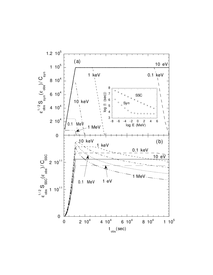
Figure 1: Synchrotron (Fig. 1a) and SSC (Fig. 1b) fluxes as a function of time at different photon energies. Nonthermal electrons with injection index $s=2$ are injected for $\Delta t=10^{5}$ seconds into a spherical plasmoid at redshift $z=0.1$, and with Doppler factor ${\cal D}=10$ with respect to the observer. Other parameters are given in the text. The mean time of the fluxes as a function of observer energy, defined by equation (8), are shown in the inset.

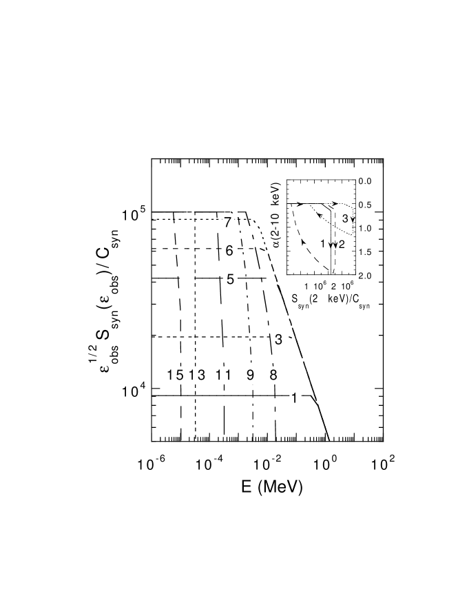
Figure 2: Synchrotron fluxes as a function of observing energy at different observing times $t_{\rm obs}({\rm s})=[(1+z)\Delta t/{\cal D})]\times 10^{(j-7)/6}$, using the same parameters as in Figure 1. The curves are labeled by $j$. The inset shows the tracks followed by the 2-10 keV spectral index versus a quantity proportional to the 2 keV spectral flux. Various levels of background fluxes, as described in the text, are included in the calculations of the dashed and dotted curves.

References

- (1) Bloom, S. D., et al. 1997, ApJ, 490, L145
- (2) Buckley, J. H. et al. 1996, ApJ, 472, L9
- (3) Buckley, J. H. et al. 1998, Adv. Space Research, 21, 101
- (4) Catanese, M., et al. 1997, ApJ, 487, L143
- (5) Chiang, J., & Dermer, C. D. 1998, ApJ, submitted (astro-ph 9803339)
- (6) Dermer, C. D., & Chiang, J. 1998, New Astronomy, 3, 157
- (7) Dermer, C. D., Sturner, S. J., & Schlickeiser, R. 1997, ApJS, 109, 103
- (8) Dermer, C. D. 1995, ApJ, 446, L63
- (9) Fenimore, E. E., In’t Zand, J. J. M., Norris, J. P., Bonnell, J. T., & Nemiroff, R. J. 1995, ApJ, 448, L101
- (10) Fenimore, E. E., Madras, C., & Nayakshin, S. 1996, ApJ, 473, 998
- (11) Fishman, G., et al. 1992, in Gamma-Ray Bursts: Huntsville, 1991, ed. W. S. Paciesas & G. J. Fishman (New York: AIP), 13
- (12) Hartman, R. C., et al. 1996, ApJ, 461, 698
- (13) Hurley, K. C., et al. 1994, Nature, 372, 652
- (14) Idesawa, E., et al. 1997, PASJ, 49, 631
- (15) Kirk, J. G., Rieger, F. M., & Mastichiadis, A. 1998, A&A, in press (astro-ph 9801265)
- (16) Kazanas, D., Titarchuk, L. G., & Hua, Xin-Min 1998, ApJ, 493, 708
- (17) Liang, E. P., & Kargatis, V. 1996, Nature, 381, 49
- (18) Link, B., Epstein, R. I., & Priedhorsky, W. C. 1993, ApJ, 408, L81
- (19) Macomb, D. J. et al. 1995, ApJ, 449, L99; (e) 1996, ApJ, 459, L111
- (20) Mészáros, P., Rees, M. J., & Papathanassiou, H. 1994, ApJ, 432, 181
- (21) Norris, J., et al. 1986, ApJ, 301, 213
- (22) Piro, L., et al. 1998, A& A, 329, 906
- (23) Reynolds, S. P. 1991, in Testing the AGN Paradigm, ed. S. S. Holt, S. G. Neff, & C. M. Urry (New York: AIP), 455
- (24) Sembay, S., et al. 1993, ApJ, 404, 112
- (25) Shrader, C. R., & Wehrle, A. E. 1997, in The Fourth Compton Symposium, ed. C. D. Dermer, M. S. Strickman, & J. D. Kurfess (New York: AIP), 328
- (26) Takahashi, T., et al. 1996, ApJ, 470, L89
- (27) Tashiro, M., Makishima, K., Ohashi, T., Inda-Koide, M., Yamashita, A., Mihara, T., & Kohmura, Y. 1995, PASJ, 47, 131
- (28) Tavani, M. 1996, ApJ, 466, 768
- (29) Vietri, M. 1997, ApJ, 478, L9
- (30) Wagner, S. J. 1997, in Relativistic Jets in AGN, ed. M. Ostrowski et al., (Kraków: Poligrafia ITS), 208
- (31) Waxman, E. 1997, ApJ, 485, L5