Morphology of Clusters and Superclusters in N-body simulations of Cosmological Gravitational Clustering

Abstract

We analyse shapes of overdense regions (clusters and superclusters) in controlled N-body simulations of gravitational clustering with power law initial spectra $P(k)\propto k^{n}$, $n=-3,-2,-1,0.$ At values of the density just above the percolation transition the number of distinct (isolated) clusters peaks and we use this ‘natural threshold’ to study the shapes and multiplicity function of clusters & superclusters. We find that the extent of both filamentarity and pancakeness increases as the simulation evolves, the former being appreciably larger than the latter at virtually all epochs and for all spectra considered by us. Our results also show that high density regions within very massive clusters/ superclusters are likely to be noticeably filamentary or pancake/ribbon-like when compared to the less dense regions within these objects. We make a detailed study of two, moment-based ‘shape statistics’ proposed, respectively, by Babul & Starkman (BS) and Luo & Vishniac (LV) and find that both LV and BS have certain built-in limitations: LV is biased towards oblate structures and tends to overemphasise this property; neither BS nor LV correctly describe the shape of strongly curved or topologically nontrivial objects. For instance, a thin filamentary torus and a ribbon are both described by BS and LV as being pancakes ! By contrast Shapefinders, a new shape diagnostic not constructed from density moments but from Minkowski functionals, does not suffer from these limitations and appears to faithfully reproduce the shapes of both simple and topologically complex objects.

1 INTRODUCTION

Large angle redshift surveys appear to confirm that, far from being randomly distributed, galaxies are clustered and appear to form a cellular/filamentary network consisting of clusters and superclusters of galaxies which are separated from each other by large voids. The clustering properties of galaxies have been successfully studied by means of statistical indicators such as the two-point correlation function, the probability density function, etc. ([Sahni & Coles 1995]). Useful as these indicators are, they say very little about the large scale texture of the galaxy distribution or its morphology. Such questions are meaningful since, as demonstrated in a variety of numerical experiments, galaxies can mesh together in a number of distinct ways, which could be suggestive of a “meatball” topology, “sponge” topology, “bubble” topology, etc. ([de Lapparent, Geller, & Huchra 1991, Gott, Melott, & Dickinson 1986, Gott et al. 1987, Melott 1990, Yess, Shandarin & Fisher 1997]). In addition, the presence of spectacular large scale features in galaxy catalogues such as “great walls” in the combined CfA-SSRS surveys, begs the question as to whether such features are one-dimensional “filaments” or two-dimensional “pancakes/ribbons”.

The shapes (and topologies) of individual clustered objects are important quantities which are bound to shed light on physical processes responsible for galaxy clustering. In the so-called ‘standard model’, wherein clustering is driven by gravitational instability and the initial perturbations are assumed to be smooth, conventional wisdom is that the first nonlinear objects to form are likely to be ‘pancakes’ (Zel’dovich 1970, Shandarin et al. 1995). However, as recent work has emphasised, the density distribution comes to be dominated by filaments which weave nearby clusters into a ‘cosmic web’ (Bond, Kofman & Pogosyan 1996). There is no contradiction between these statements. They simply stress different aspects of nonlinear distributions. The former simply describes the shape of the first caustics. The latter stresses the fact that in a smoothed density field (caustics must not be present) the percolation threshold from disconnected clumps to connected structure (in other words from the meatball to sponge topology), occurs at a higher density threshold than the other percolation transition from the sponge topology to the bubble topology. This is correct for every generic field. As gravitational clustering advances, filamentarity increases and planarity too remains statistically significant (Sathyaprakash, Sahni & Shandarin 1996). Thus, the Universe during late stages of gravitational clustering (hierarchical clustering or hierarchical pancaking, see e.g., [Coles, Melott & Shandarin 1993]) consists of a variety of geometrical objects, whose shape and relative abundance are likely to depend both upon the initial spectrum of density perturbations and upon the epoch at which clustering is being studied. Other scenario’s of structure formation in which large scale structure is formed by cosmological explosions or seeded by topological defects (strings, textures) will undoubtedly predict a different evolution for clustering and hence also a different morphology for the clustered objects.

Strictly speaking, idealised Zel’dovich pancakes form locally, and whether or not coherence exists over large scales so that the first objects form as large sheets of matter, depends largely upon the primordial fluctuation spectrum. Moreover, since Zel’dovich pancakes are transient features which arise when first caustics form, it is not likely that matter will still be organised in two-dimensions during the later, strongly non-linear stages of gravitational instability. Finally, although formally the density in a Zel’dovich pancake is infinite, in a realistic situation pancakes are expected to be of finite density — less dense than filaments since collapse is along a single dimension for pancakes, whereas filaments form by the two-dimensional collapse of matter (Shandarin & Zeldovich 1989). Thus, filaments are likely to be more prominent than pancakes, as has indeed been observed and quantified for N-body simulations (Klypin & Shandarin 1993; Sathyaprakash et al. 1996). The above examples illustrate that it is necessary to address the evolving morphology of large scale structure by using good statistical indicators. Simple methods, such as fitting an ellipsoid to a cluster of galaxies, could lead to an erroneous picture, since structures found in surveys need not have any definite archetypal structure implicitly assumed in such methods. Also, the morphology of structure often depends on scale. Therefore, one needs more refined scale dependent statistical tools with which to study morphology.

In this study, we analyse the morphology of overdense regions arising as a result of gravitational instability using some recently suggested statistical tools. We study the three-dimensional ‘structure functions’ introduced by Babul and Starkman (1992) and also consider an alternate shape statistic proposed by Luo and Vishniac (1995). We apply these discriminators to study overdense regions (clusters & superclusters) in scale-invariant N-body simulations for varying epochs of nonlinearity and different initial spectra. The present work extends previous work on the subject including that of Dubinsky (1992) who used ellipsoid-fitting to study the shapes of individual density peaks as they evolved under gravitational instability. A one-dimensional shape statistic originally proposed by Vishniac (1986) has been used to study the growth of filamentarity in two-dimensional simulations of gravitational clustering by Nusser & Dekel (1990) and Sathyaprakash et. al. (1995). More recently, a shape statistic based on spatial links between high density regions was discussed in [Davé et al. 1997]; Sahni, Sathyaprakash & Shandarin (1998) proposed a new shape diagnostic based on Minkowski functionals. Our present analysis also extends work by Sathyaprakash et. al. (1996) to later nonlinear epochs using a wider range of initial conditions and more robust and sensitive shape statistics. Our results indicate that: (i) the shape of overdense regions evolves with time, (ii) with the development of nonlinearity both filamentary and pancake-like properties of individual clusters are enhanced and (iii) individual objects get progressively more filamentary than planar as the simulation evolves. These general results hold for a wide range of initial conditions and appear to be generic features of structure formation scenario’s driven by gravitational instability. However, quantitatively speaking, though all spectra initially produce small filaments and pancakes, at later epochs spectra with steeper (negative) slope produce larger filaments and pancakes, the former being more prominent. In this study we shall not confine ourselves to studying peaks of the density field, rather, we shall apply shape statistics to all regions above a given density threshold and study shapes of isolated objects as well as the morphology of large scale structure as a whole. We shall use percolation analysis to aid us in determining a suitable density threshold above which to identify clusters.

2 N-BODY SIMULATIONS

The N-body simulations used in our study are produced by a staggered particle-mesh code with 128³ particles on a 128³ mesh and a corresponding Nyquist wavenumber, $k_{\rm Ny}=64.$ The initial conditions are generated by the Zel’dovich approximation (Klypin & Shandarin 1983 ) such that the initial power spectrum is a simple power-law covering the range $n=0,-1$, $-2$ and $-3$. The models are allowed to evolve gravitationally until nonlinear effects change the slope of the power spectrum. This change indicates that phase correlations have developed between the originally random initial phases. The extent of nonlinearity can be characterised by the parameter $k_{\rm nl},$ defined by the equation $\sigma_{\delta}=a^{2}\int_{0}^{k_{\rm nl}}P(k)d^{3}k=1,$ where $P(k)$ is the power spectrum of fluctuations. In this study, we evolve the simulations to values of $k_{\rm nl}=64,32,16,8,$ and $4.$ The value of $k_{\rm nl}$ relates to the scale of structure formation in real space. For a detailed discussion of the N-body simulations see Melott & Shandarin (1993).

In our study of shapes of clusters we only use density fields. Density fields are derived from the above simulations by a cloud-in-cell method, whereby each particle’s mass is proportionately spread over a $2^{3}$ cell-volume and rescaled (8:1) to produce a $64^{3}$ density field. This method implies some smoothing at small scales but reduces shot noice so that further smoothing is not needed before any analysis. An ensemble family of four realisations is produced from each combination of $n$ and $k_{\rm nl}$ to give assessments of the one-$\sigma$ level dispersion for each physical quantity measured.

It is likely that no single model studied can pretend to explain the real universe. We consider them to be toy models that serve as a good test-bed for our shape statistics. However, if one wishes to get a rough idea of how they may relate to the real world we provide the following normalisations. We assume that the rms fluctuation in number of galaxies is about unity within spheres of radius $8h^{-1}$ Mpc, the rms mass density fluctuation $\sigma_{m}$ is parameterised by the “bias factor”, $b,$ such that $\sigma_{g}=b\sigma_{m}$. We shall assume that $b\simeq 1$ which is an adequate assumption for these crude estimates. Melott & Shandarin (1993) showed that, for the models in question, the scale of nonlinearity, measured by the top-hat smoothing filter, $R_{\rm TH},$ is approximately two times greater than $k_{\rm nl}^{-1},$ calculated from the extrapolation of linear theory (more accurately: $R_{\rm TH}\simeq 1.8k_{\rm nl}^{-1}$ in the $n=0,-1$ models and $R_{\rm TH}\simeq 2.8k_{\rm nl}^{-1}$ in the $n=-2$ model). Thus, identifying every stage with the present time one can roughly estimate the size of a mesh cell: $l_{c}\simeq 26h^{-1},$ $12.6h^{-1},$ $6.3h^{-1},$ $3.1h^{-1}$ and $1.6h^{-1}$ Mpc for $k_{\rm nl}=64,32,16,8$ and $4$, respectively. In our models the smoothing has been performed with a top-hat filter having a cubic rather than spherical shape which may add an additional factor of $(4\pi/3)^{-1/3}=0.6$ (assuming volumes of the filters are similar: $l_{c}^{3}=(4\pi/3)(R_{\rm TH}^{(s)})^{3}).$ Therefore, one can view each stage of evolution of the models as the density distribution seen after smoothing with a top-hat filter of radius $R_{\rm TH}^{(s)}\simeq 16h^{-1},~{}8h^{-1},~{}4h^{-1},~{}2h^{-1},$ and $1h^{-1}$ Mpc within box-volumes of $(64l_{c})^{3}\simeq(1600h^{-1}{\rm Mpc})^{3},$ $(800h^{-1}{\rm Mpc})^{3},$ $(400h^{-1}{\rm Mpc})^{3},$ $(200h^{-1}{\rm Mpc})^{3}$ and $(100h^{-1}{\rm Mpc})^{3}$, for $k_{\rm nl}=64,$ 32, 16, 8 and 4, respectively.

The purpose of these estimates is to give a rough idea of the range of parameters characterising models, and therefore more elaborate calculations are probably not needed. (More realistic models will be discussed in Sathyaprakash, Sahni, Shandarin & Ryu 1998.)

3 METHODS OF ANALYSIS

In this Section we briefly describe the statistical tools employed by us to characterise the morphology of large scale structure (LSS). We introduce the Babul & Starkman and Luo & Vishniac shape statistics and also describe in detail our method of identifying individual clusters at a density threshold prescribed by percolation theory.

3.1 Shape Statistics

In order to quantify the morphology of structure, both of isolated clusters and of LSS as a whole, we use suitably modified versions of the structure functions introduced by Babul & Starkman (1992) as also the shape statistics of Luo & Vishniac (1995). These authors define the morphology of the distribution of particles by constructing the first- and second-moments of the particle distribution around a given point. Geometrically, the shape and structure functions are nonlinear transformations of the three eigenvalues of the ellipsoid “fitted” to the distribution of particles around the given point. These transformations are implemented so as to suitably tune and normalise the parameters describing morphology and to factor out the size of the distribution, which does not play a role in describing ‘shape’. Both ‘shape statistics’ and ‘structure functions’ are described by a doublet consisting of two numbers, the first describing filamentarity (or prolateness) and the second characterising planarity (or oblateness). (Babul and Starkman do use a triad, however the presence of a single non-linear functional relationship between members of the triad makes only two of them independent.) It is interesting that, for an object chosen randomly from our N-body simulations, both shape statistics do not usually give identical results, a feature to which we shall return in later sections !

As we shall demonstrate, these measures of filamentarity and planarity do not always reflect the visual shape of an object. This may be because, although the nomenclature filaments/pancakes is perfectly valid for extreme cases e.g. matter spread along an infinitely thin line or in an infinitely thin plane, one has to be careful in interpreting the values measured by these moment-based shape statistics when we are dealing with objects which are neither prefectly planar nor perfectly linear. The fact that the moments of a distribution do depend on the choice of origin makes things even more complicated and we shall have more to say about this and related issues when we discuss shape eikonals in Section 4 We shall see there that the Luo-Vishniac shape statistics has the drawback that it is biased towards planarity and is therefore not a good statistical measure of morphology despite being derived in a mathematically rigorous and appealing manner.

3.2 Global and Local Morphology

Conventionally, one studies the morphology of LSS by placing windows of increasingly larger size centered on randomly chosen points and averaging over many such sample points. However, a certain amount of control should be exercised in the choice of sample points so as to reduce the inevitable scatter in the signal. Since our interest is mainly to study the morphology of galaxy clusters and superclusters we can achieve this by choosing only those random points where the density is larger than a preset threshold. Such a study of average morphology is very useful in establishing an overall picture. However, in order for the shape statistics to be useful in discriminating models of structure formation and to address issues relating to the physics of gravitational instability it is appropriate to study the morphology of individual objects, the shape distribution function, dependence of shape on cluster mass and size, etc. In studying the morphology of individual objects one has several options and care has to be exercised in making a choice. For instance, we can use either the centre of mass to be the origin or the geometrical centre; we can enclose the whole object in a window of size larger than the object or study its shape as a function of window size starting with a small window centered around the origin. We could either weigh the shape functions with the local value of the density or choose not to weigh them. Each of these methods has its own merit and yields information complementary to the others. The study of morphology of individual objects can therefore be very rewarding and rich in information content.

It is also important to study the morphology of structure at different density thresholds since one and the same object will generally exhibit different properties at varying thresholds. For example, at very high density or brightness thresholds a barred spiral galaxy surrounded by a dark halo would look filamentary, at moderate densities a disc and at very low densities a spheroid. Therefore, in this work we not only study the global morphology of structure but also the morphology of isolated clusters and superclusters at different density thresholds.

3.3 Identifying Structures using Percolation Theory

The issue of density threshold mentioned earlier can bring forth an element of subjectivity into the analysis and the resulting picture can be confusing if density thresholds are chosen in an arbitrary manner. We try to introduce some objectivity in choice of threshold by using percolation analysis, which is a tool to understand connectivity of structure and hence is closely linked to the study of morphology.

Our method of identifying structures is the following: at any given density threshold a cluster is defined using a ‘friends-of-friends’ algorithm with six nearest neighbours. At very high thresholds only a small volume is in the overdense phase, consequently there are very few clusters and the largest of them is very small. As the density threshold is lowered the overdense phase grows, leading to an increase in the number of clusters and a concomitant growth in the volume (and mass) of the largest cluster. Indeed, lowering the density contrast further causes many small clusters to merge with the largest cluster, leading to a sharp increase in the volume of the latter until, at the percolation transition, the largest cluster runs across the entire region of interest and has a volume which is a significant fraction $(>10\%$) of the total volume in the overdense phase. It turns out that the number of distinct clusters is most abundant just before the percolation transition which leads us to feel that the percolation threshold provides a natural choice at which to identify structures (see Fig. 1). We also use other thresholds in addition to percolation (see below) at which to identify clusters, demonstrating in the process, that the main conclusions of this study are not sensitive to choice of threshold. (Other aspects of percolation theory are discussed in [Yess & Shandarin 1996, Sahni, Sathyaprakash & Shandarin 1997].)

We now introduce the shape statistics used in our study.

3.4 The Babul-Starkman Statistic

Let $\vec{x}^{p}=(x^{p}_{1},x^{p}_{2},x^{p}_{3}),$ $p=1,\ldots,N,$ denote the position vector of the $p$th particle in a system consisting of $N$ particles. The first- and second-moments of the particle distribution around a fiducial point $\vec{x}^{0}$ are given by

$$M_{i}(\vec{x}^{0};R) = \frac{1}{N}\sum_{p=1}^{N}\left(x^{p}_{i}-x^{0}_{i}\right)W\left(|\vec{x}^{p}-\vec{x}^{0}|\right),$$

$$M_{ij}(\vec{x}^{0};R) = \frac{1}{N}\sum_{p=1}^{N}\left(x^{p}_{i}-x^{0}_{i}\right)\left(x^{p}_{j}-x^{0}_{j}\right)W\left(|\vec{x}^{p}-\vec{x}^{0}|\right),$$ (1)

where $i,j=1,2,3$ and $W$ is a window of effective radius $R$ centred on the point $\vec{x}^{0}$. The moments do, in general, depend on the nature of the window function. In this study, we use a simple spherical window function. Given the moments of the distribution one can compute the moment of inertia tensor $I_{ij}$

$$I_{ij}=M_{ij}-M_{i}M_{j}.$$ (2)

The three eigenvalues $I_{1},$ $I_{2}$ and $I_{3},$ of the inertia tensor represent the three principal axes of an ellipsoid fitted to the matter distribution around the point in question, they therefore contain information about how the matter is distributed around a given point. (This statement is rigorously true if $R$ is infinitesimally small making it possible for the density field about a local maximum to be approximated by a quadratic, which in turn, is equivalent to fitting by an ellipsoid.) The absolute value of the eigenvalues is not important in quantifying morphology and therefore it suffices to consider their ratios

$$\mu\equiv\left(\frac{I_{2}}{I_{1}}\right)^{1/2},\ \ \nu\equiv\left(\frac{I_{3}}{I_{1}}\right)^{1/2},$$ (3)

where we assume that eigenvalues are arranged in order of increasing magnitude, i.e., $I_{1}\leq I_{2}\leq I_{3}.$ The shape statistic of Babul & Starkman (1992) (henceforth BS) consists of a triad of numbers $(S_{1},S_{2},S_{3})$ and is constructed out of the parameters $\mu$ and $\nu$ as follows:

$$S_{1} = \sin\left[\frac{\pi}{2}\left(1-\mu\right)^{p}\right],$$

$$S_{2} = \sin\left[\frac{\pi}{2}a(\mu,\nu)\right],$$

$$S_{3} = \sin\left[\frac{\pi}{2}\nu\right],$$ (4)

where $p=\log 3/\log 1.5,$ the function $a(\mu,\nu)$ is implicitly given by

$$\frac{\mu^{2}}{a^{2}}-\frac{\nu^{2}}{a^{2}(1-\alpha a^{1/3}+\beta a^{2/3})}=1,$$ (5)

and the parameters $\alpha$ and $\beta$ are defined by

$$\alpha=1.9,~{}\beta=-\frac{7}{8}9^{1/3}+\alpha 3^{1/3}.$$ (6)

These definitions ensure $0\leq S_{i}\leq 1$, $i=1,2,3$ and $|\vec{S}|\leq 1$ for the ‘shape vector’ $\vec{S}=(S_{1},S_{2},S_{3}),$ which, therefore, always lies in the first octant of a three-dimensional ‘shape-space’.

The set of all shape vectors (points associated with the tip of the shape vector) spans a three dimensional volume, every point located within this volume corresponding to a certain geometrical shape. For a spherical distribution we have $I_{1}=I_{2}=I_{3}$ which implies that $\mu=\nu=1$ and $a=0$ so that $(S_{1},S_{2},S_{3})=(0,0,1).$ For a planar distribution $I_{1}=I_{2},$ $I_{3}=0$ which implies $\mu=1,$ $\nu=0$ and $a=1$ so that $(S_{1},S_{2},S_{3})=(0,1,0).$ Finally, for a linear distribution $I_{2}=I_{3}=0$ so that $\mu=\nu=a=0$ and $(S_{1},S_{2},S_{3})=(1,0,0).$ Consequently, BS call $S_{1}$ filamentarity, $S_{2}$ planarity and $S_{3}$ sphericity. For a distribution of matter which is neither perfectly spherical nor planar nor linear: $S_{i}\neq 0$, $i=1,2,3.$ In such cases it is best not to use any qualifying words to describe structure but speak in terms of the magnitude and orientation of the shape vector. From (4) – (6) one finds that $S_{1}$, $S_{2}$, $S_{3}$ are not independent, a knowledge of any two of them effectively determines the third. We shall work with $S_{1}$ and $S_{2}$ whose maximum values characterise a filament and a pancake respectively; small values of both $S_{1}$ and $S_{2}$ imply a large sphericity ($S_{3}$) for the distribution.

Clearly, the moments as defined above are only useful for point processes and cannot be used if we want to address the morphology of continuous distributions such as density fields, surface brightness, etc. We therefore need to generalise these concepts to fields defined in space. This can easily be accomplished by defining density-weighted moments as follows

$$M_{i}(\vec{x}^{0};R) = \frac{1}{\cal M}\sum_{p=1}^{N}\left(x^{p}_{i}-x^{0}_{i}\right)\rho\left(\vec{x}^{p}\right)W\left(|\vec{x}^{p}-\vec{x}^{0}|\right),$$

$$M_{ij}(\vec{x}^{0};R) = \frac{1}{\cal M}\sum_{p=1}^{N}\left(x^{p}_{i}-x^{0}_{i}\right)\left(x^{p}_{j}-x^{0}_{j}\right)\rho\left(\vec{x}^{p}\right)W\left(|\vec{x}^{p}-\vec{x}^{0}|\right),$$ (7)

where $i,j=1,2,3,$ and $\cal M$ is the total mass in the region of interest:

$${\cal M}=\sum_{p=1}^{N}\rho\left(\vec{x}^{p}\right)W\left(|\vec{x}^{p}-\vec{x}^{0}|\right).$$ (8)

substituting (7) in (2) – (4) we obtain ‘structure functions’ $\vec{S}=(S_{1},S_{2},S_{3})$ defined for a continuous density field.

Since $\rho$ could, in principle, be an arbitrary scalar quantity it is clear that the shape statistic can now be computed for any scalar field, be it a density field, surface brightness, temperature field, etc., this useful modification allows us to apply shape statistics to a wider variety of situations.

3.5 The Luo-Vishniac Statistic

The BS statistic is derived heuristically and (we guess) by experimenting with the behaviour of the shape vector as different parameters, such as $p,$ $\alpha$ and $\beta$ are varied. Luo and Vishniac follow a more rigorous approach. The starting point for their shape statistic is once again the moments of the distribution. They introduce a shape function which is the most general and coordinate-independent linear combination of the moments of cubic non-linearity:

$$S(R) = \frac{1}{M^{3}}\biggl{[}aM\left(M_{ij}-M_{i}M_{j}\right)\left(M_{ij}-M_{i}M_{j}\right)+bM\left(M-M_{i}M_{i}\right)^{2}+\biggr{.}$$ (9)

$$\biggl{.}cM_{ij}\left(M_{ik}-M_{i}M_{k}\right)\left(M_{jk}-M_{j}M_{k}\right)+dM_{ij}\left(M_{ij}-M_{i}M_{j}\right)\left(M-M_{k}M_{k}\right)\biggr{]},$$

where a summation over repeated indices is implied. As earlier $R$ is the radius of the window function, $M=M_{ii}$ is the trace of the second-moment, and $a$, $b,$ $c,$ and $d$ are constants. The constants $a,$ $b,$ $c$ and $d$ can be determined by demanding that the geometrical construct $S(R)$ be consistent with what we intuitively expect for the morphology of archetypal point distributions. By requiring that the shape function vanish for a uniform distribution of particles within the region of interest one obtains two constraints which fix two out of the four constants. In order to fix the remaining two one can either demand that the shape function be unity for an infinitely thin linear distribution and zero for an infinitely thin planar distribution or vice versa. In the first case one obtains the statistic $S_{l}$ and in the second case one obtains $S_{p},$ which Luo and Vishniac call linearity and planarity, respectively:

$$S_{l}\equiv S(R),a=-1,\ b=1/2,\ c=3,\ d=-3/2$$ (10)

$$S_{p}\equiv S(R),a=4,\ b=-4,\ c=-12,\ d=12.$$ (11)

Thus, the Luo-Vishniac statistic (henceforth LV) consists of a doublet of numbers $S_{l}$ and $S_{p}$ both of which satisfy $0\leq S_{l},S_{p}\leq 1.$

Having introduced the BS and LV shape functions we now proceed to test their effectiveness in determining shapes.

4 Shape Eikonals

In this Section we address the following questions related to the internal consistency and robustness of the shape statistics: (i) is the statistic a good measure of morphology and consistent with the visual impression conveyed by a structure? (ii) is the statistic unbiased? The important related issue of whether the statistic performs reasonably well in the presence of noise, has been amply addressed by BS and LV who concluded that the statistic they had proposed was reasonably robust. We return to this issue in a future work when we shall address the performance of different shape statistics in the presence of noise ([Buchert, Sathyaprakash, Schmalzing & Sahni 1998]). For the present we investigate whether the BS and LV shape statistics correctly diagnose the shape of an object.

Our first aim is to test the performance of shape statistics using different eikonal shapes for this purpose. (i) We study the behaviour of the shape statistics as a sphere is continuously deformed into an oblate or prolate ellipsoid and describe this behaviour using trajectories in ‘shape phase-space’ representing continuous deformations; (ii) we study the morphology of objects with a non-trivial topology, such as a torus, this study leads to an important conclusion, namely, descriptions of morphology (of LSS) are incomplete if only moment-based shape statistics are used, the latter must be supplemented with shape diagnostics sensitive to topology (Sahni, Sathyaprakash & Shandarin 1998); (iii) we randomly choose isolated structures (clusters/superclusters) from an N-body simulation and apply the BS and LV statistics to study their shapes. This permits us to say something about the extent of the shape phase-space sampled, respectively, by BS and LV.

4.1 Structural Transformations and ‘Shape-Space’

As mentioned in the last Section, the doublets $(S_{l},~{}S_{p})$ and $(S_{1},~{}S_{2})$ can be treated as two-dimensional vectors with norm $\leq 1$. The following questions then arise: given an ensemble of geometrical objects what possible values could these vectors take? In other words what is the shape phase-space sampled by the two statistics? To explore this in a heuristic way we consider geometrical transformations of a sphere into oblate and prolate ellipsoids ([Babul & Starkman 1992]). (Henceforth we shall refer to shape phase-space as simply shape-space.)

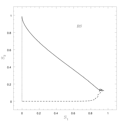
Figure 2: Structural deformations of a sphere: sphere $\rightarrow$ pancake (dotted line), pancake $\rightarrow$ filament (solid line) and filament $\rightarrow$ sphere (dashed line), are illustrated in the form of a ‘shape phase-space’ for the Babul-Starkman statistics ($S_{2}$ versus $S_{1}$, left panel) and Luo-Vishniac statistics ($S_{p}$ versus $S_{l}$, right panel).

Let $r_{x}\geq r_{y}\geq r_{z}$ denote the three principal radii of an ellipsoid. Since the size of the object is unimportant let us fix one of the radii, say $r_{x},$ to unity. In Fig. 2 we have plotted $S_{2}$ vs $S_{1}$ and $S_{p}$ vs $S_{l},$ as a sphere ($r_{x}=r_{y}=r_{z}=1$) with $(S_{1},S_{2})=(S_{l},S_{p})=(0,0)$, is continuously deformed either into an oblate ellipsoid ($r_{x}=r_{y}=1,0\leq r_{z}\leq 1$) ending up in a plane ($r_{z}=0$) with $(S_{1},S_{2})=(S_{l},S_{p})=(0,1);$ or into a prolate spheroid ($r_{x}=1,r_{y}=r_{z},$ $0\leq r_{y},r_{z}\leq 1$) ending in a line ($r_{y}=r_{z}=0$), with $(S_{1},S_{2})=(S_{l},S_{p})=(1,0).$

First consider the BS statistic. As the sphere is continuously deformed into a plane, $S_{2}$ (planarity) increases from 0 to 1, while $S_{1}$ (filamentarity) remains zero throughout. Similarly, as the sphere is deformed into a line, $S_{2}$ remains fixed at zero while $S_{1}$ increases from 0 to 1 (cf. Fig. 2 left panel). (During these deformations $S_{3}$ (sphericity) decreases from 1 to 0.) Such a behaviour has been made possible by a proper tuning of parameters ($p,$ $\alpha$ and $\beta$ in Eqs. (4) and (5)) in the BS statistic ([Babul & Starkman 1992]). Based on the above ‘experiment’ it is reasonable to expect that if objects of all possible shapes are analysed, the BS statistic would fill in a triangle in ‘shape-space’. (For both BS and LV statistics shape shape-space is triangular since, according to these statistics, no object can be simultaneously a pancake and a filament. However, such objects might occur in nature; for example a long ribbon has a mixed morphology of both a pancake and a filament – see Table 1.)

Next, let us consider the LV statistic. As a sphere is deformed into a plane, we find that while $S_{l}$ (linearity) remains zero, $S_{p}$ (planarity) increases from 0 to 1. However, the LV statistic shows anomalous behaviour as a sphere is deformed into a filament. Notice that for this deformation $S_{p}$ does not remain fixed at zero as $S_{l}$ increases from 0 to 1. Contrary to expectations planarity initially increases as a sphere is deformed into a filament. Consequently, shape-space is only partially filled as seen in Fig. 2b. Thus, according to this statistic, while an object can be planar without any attributes of linearity, it cannot be linear without having a measure of planarity. This anomalous behaviour demonstrates that the LV statistic is biased towards planarity and may not be a suitable tool with which to study the morphology of large scale structure. This unattractive feature, present in a statistic which in all other respects is rigorously defined, reminds us of the complexities of constructing a good shape statistic and the related difficulty in modelling and quantifying the morphology of LSS. It might be that a certain amount of parameter ‘tuning’ (as in BS) is necessary in order to obtain a good moment-based shape statistic.

4.2 Structures with non-trivial Topology

Sometimes what our mathematical constructs measure may not be consistent with the visual impression conveyed by an object. To illustrate this, consider a torus having an elliptical cross-section described by the parametric form

$${\bf{r}}=(b+c\sin{\phi})\cos{\theta}~{}\hat{x}+(b+c\sin{\phi})\sin{\theta}~{}\hat{y}+a(\cos{\phi})\hat{z}$$ (12)

$a,c<b$, $0\leq\phi,\theta<2\pi$. The torus has diameter $2\pi b$ and an elliptical cross-section, $a$ and $c$ being, respectively, radii of curvature perpendicular and parallel to the plane of the torus. The circular torus is given by $a=c$. Geometrically, an infinitely thin circular torus is one-dimensional while a sheet is two-dimensional. However, the moment of inertia about the centre of mass cannot distinguish between the two distributions, the ratios of eigenvalues of the inertia tensor, $\mu$ and $\nu,$ being exactly the same for both objects. As both BS and LV are moment based statistics, torus and sheet are declared to be sheet-like, i.e., we get $(S_{1},S_{2})=(S_{l},S_{p})=(0,1)$ for both objects!

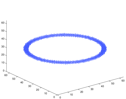
Figure 3: BS shape parameters $S_{1}$ and $S_{2}$ are shown plotted as a function of the window size for the toroidal distribution of matter shown in the upper left panel. The window is located at the centre-of-mass in (a) and at a point enclosed by the surface of the torus in (b). In (c) average values of $S_{1}$ and $S_{2}$ are computed using a number of random points.

We therefore see that if we were to study shape statistics with moments evaluated about the centre of mass, sometimes we could get a spurious result. For a torus this arose because the torus does not enclose its centre of mass within itself. This problem can be partially alleviated by determining the moments about a point enclosed by the surface of the torus, rather than about its centre of mass. If we do this then, for small sizes of the window, the statistics do declare the torus to be a filament (i.e. $S_{1}\simeq 1$ and $S_{2}\simeq S_{3}\simeq 0$). However, as the window radius gets larger, filamentarity reduces and planarity increases, till the torus is once more declared to be a planar object ($S_{1}\simeq S_{3}\simeq 0$ and $S_{2}\simeq 1$) when the size of the window exceeds the radius of the torus. Another method which might yield sensible results would be to average the shape statistics by choosing a number of different points in a window that completely encloses the object. This would declare the torus to be an intermediate object having both filamentary and planar properties. To illustrate these different methods we consider a circular torus which is shown in the upper-left corner of Fig. 3. The BS statistics $S_{1}$ (solid-line) and $S_{2}$ (dashed-line) are plotted as functions of the size $R$ of the window centred at (a) the centre-of-mass (upper-right) and (b) a random point on the torus (lower-left). We also show averaged BS statistics obtained by choosing (c) a number of random centres in the region enclosing the torus (lower-right). (The LV statistics give similar results and we do not show them here.)

Of course, it is unlikely that in any simulation or survey one will find a perfect torus; nor for that matter is one likely to find a perfect filament or sheet. In cases where the matter distribution is one-dimensional, but not along a straight line, one is bound to get a somewhat smaller signal for filamentarity from both BS and LV than if the distribution is perfectly straight. This is even more true for two-dimensional distributions: An infinitesimally thin spherical shell and a distribution which is isotropic about a given point have identical moments about their centres and will be declared ‘spherical’ by both BS and LV. Similarly, wiggly, wavy or bent two-dimensional surfaces will not be declared sheets by these statistics; i.e., $S_{2},S_{p}\neq 1$. Moreover, as predicted by the Zeldovich approximation and the adhesion model, cosmological pancakes are not as prominent as filaments or clumps nor are they likely to be perfectly flat, planar objects. This makes it difficult for moment-based shape-statistics to detect pancakes in N-body simulations and in galaxy surveys. Problems such as these have prompted us to explore other statistics to describe morphology which not only take into account shape but topology of structure as well. Shapefinders – shape diagnostics constructed from fundamental properties of a surface, such as its Minkowski functionals which we describe below, is an example of a statistic which can successfully diagnose shapes of topologically simple and complicated surfaces, without fitting them with ellipsoids (for details see Sahni, Sathyaprakash and Shandarin 1998; Minkowski functionals are discussed in [Mecke et al. 1994]).

Shapefinders for a compact surface (which could be an isodensity surface in simulations or surveys) are constructed from the following four ‘Minkowski functionals’ : (i) Volume $V$, (ii) surface area $S$, (iii) integrated mean curvature: $C={1\over 2}\int(\kappa_{1}+\kappa_{2})dS$, (iv) integrated Gaussian curvature (genus): ${\cal G}=-{1\over 4\pi}\int\kappa_{1}\kappa_{2}dS,$ where $\kappa_{1}\equiv 1/R_{1}$, $\kappa_{2}\equiv 1/R_{2}$ are the principal curvatures at a point on the surface. Multiply-connected surfaces have ${\cal G}\geq 0$ while simply connected have ${\cal G}<0$.

The three Shapefinders having dimensions of [Length] are: ${\cal H}_{i},i=1,2,3,$ where ${\cal H}_{1}=V/S$, ${\cal H}_{2}=S/C$ and ${\cal H}_{3}=C$ (for multiply-connected surfaces $C/{\cal G}$ may be more appropriate than $C$). We can also define a pair of dimensionless Shapefinders : ${\bf{\cal K}}\equiv({\cal K}_{f},{\cal K}_{p})$

$${\cal K}_{p}=\frac{{\cal H}_{2}-{\cal H}_{1}}{{\cal H}_{2}+{\cal H}_{1}},\ \ {\cal K}_{f}=\frac{{\cal H}_{3}-{\cal H}_{2}}{{\cal H}_{3}+{\cal H}_{2}}.$$ (13)

where ${\cal K}_{p,f}\leq 1$ by construction. For a pancake (quasi-two-dimensional object which can be curved) ${\cal H}_{1}\ll{\cal H}_{2}\simeq{\cal H}_{3}$ and ${\cal K}_{p}\gg{\cal K}_{f}$; an ideal pancake has ${\bf{\cal K}}\simeq(0,1)$. A filament (a quasi-one-dimensional object, not necessarily straight) has ${\cal H}_{1}\simeq{\cal H}_{2}\ll{\cal H}_{3}$ and ${\cal K}_{f}\gg{\cal K}_{p}$; an ideal filament has ${\bf{\cal K}}\simeq(1,0)$. For a sphere ${\cal H}_{1}\simeq{\cal H}_{2}\simeq{\cal H}_{3}$ and ${\bf{\cal K}}\simeq(0,0)$. An additional surface to consider is a ‘ribbon’, for which ${\cal H}_{1}\ll{\cal H}_{2}\ll{\cal H}_{3}$ and ${\cal K}_{f}\sim{\cal K}_{p}>0$; an ideal ribbon has ${\bf{\cal K}}\simeq(1,1)$.

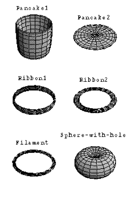
Figure 4: Deformations of a torus with elliptical cross-section. The values of BS, LV and Shapefinders shape statistics for the objects shown here are given in Table 1.

In Table 1 we provide values for the dimensionless Shapefinders ${\cal K}_{p,f}$ for deformations of the elliptical torus Eq. (12) shown in Fig. 4 and described in detail in Sahni, Sathyaprakash and Shandarin (1998). We also give corresponding values of the LV and BS shape statistics. Our results clearly show that: (i) both LV and BS give low values for ‘pancakeness’ (described by $S_{p}$, $S_{2}$) for a hollow circular cylinder, mistaking it for a spherical object ! (ii) a filamentary torus is described by both statistics as a pancake and (iii) a ribbon is mistaken for a pancake by both LV and BS. In all cases Shapefinders give a much better description of the shape of an object.

4.3 Random Sampling of clusters drawn from N-body simulations

In the last two Sections we have studied the performance of shape statistics using well defined ‘eikonal’ shapes. In this section we study the performance of BS and LV using objects drawn at random from N-body simulations. (A detailed investigation of Shapefinders is presently in progress, Buchert, Sathyaprakash, Schmalzing, Sahni (1998).)

In Fig. 5 we show scatter plots of both BS and LV statistics for structures randomly selected from N-body simulations at the percolation threshold. Conclusions drawn from the study of eikonal shapes are borne out in these scatter plots. BS clearly fills the entire shape-space whereas LV does not.

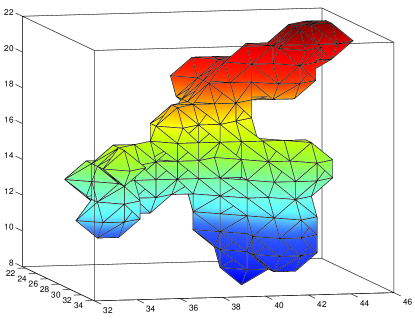
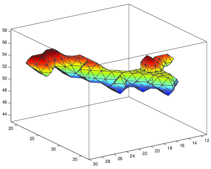
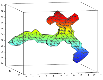
Figure 6: Some clusters (left panels) occurring in our N-body simulations are shown together with their BS & LV shape statistics as functions of window size (right panels.

In Fig. 6 we have shown three carefully selected objects chosen from our N-body simulations together with the BS statistics plotted next to them as a function of the window size. In each case the origin is chosen to be the centre of mass of the object. In (a) we show a cluster which is more planar than it is filamentary, in (b) a bent filament and in (c) we have a cluster with several tentacles emerging from it. The shape functions plotted as a function of the window size correctly reveal the morphological nature of these objects on small scales but on the scale of the object itself, the shape revealed by the statistics can occasionally be in conflict with visual impression. In the case of (c) we clearly have a collection of several one-dimensional objects joined at the centre, yet the statistics declare such an object to be planar. Perhaps this is not entirely in correct since in as the number of tentacles begins to be large we do perceive the object to be planar. However, the point is that even if we do have a fine filament, but bent, the object would acquire some degree of planarity according to both BS and LV. However, shapefinders based on Minkowski functionals are able to differentiate between a wavy filament and a planar distribution. (We would like to point out that the BS and LV statistics differ only in the value of oblateness or planarity which they attribute to a given structure, the measures of filamentarity $S_{1}$ and $S_{l}$ agree remarkably for all structures.)

Our considerations in this Section have clearly shown that the LV statistic is not suitable for the description of morphology due to its strong bias towards planarity. Consequently, in the rest of this paper we restrict its application to fewer cases than the BS statistics and rely on the latter to draw our main conclusions.

5 Evolution of cluster shape in N-body Simulations

We now apply the BS shape statistics to a systematic study of the evolution of morphology of large scale structure in N-body simulations of gravitational clustering. (Details of our N-body simulations have been discussed in Section 2) In the first part of this Section, we present a statistical analysis of our study of isolated clusters. There we discuss the shape distribution function or shape-spectrum (a plot showing the number of objects as a function of shape parameters) as well as the relationship between cluster mass and cluster shape. In the second part, we discuss the morphology of high density regions obtained by averaging shape functions over a large sample of random but high density points.

5.1 Morphology of isolated clusters in N-body simulations

We identify clusters in an N-body simulation using two different methods and evaluate the shape parameters for each case. The first method is based on percolation analysis briefly reviewed in section 3.3 The second is more elementary: we choose a density threshold such that 50% of the total mass is in high density regions. The histogram showing number of clusters obtained using the second of these methods is plotted against cluster mass in Fig. 7, for spectra with $n=-3,\ -2,\ -1,\ 0$ (left to right) and expansion epochs $k_{\rm nl}=64,\ 32,\ 16,\ 8,\ 4$ (top to bottom). (Recall that steeper spectra have more large scale power and larger $k_{\rm nl}$’s correspond to earlier epochs.) Error bars in all plots (sometimes shown as dotted lines, eg. as in Fig. 12) are computed using four independent realisations of each spectrum. For all spectra (with the possible exception of $n=-3$) we find that most of the matter gets transferred to larger clusters as the simulation evolves (presumably due to merging). Very large superclusters present during early stages are frequently not long lived objects but tend to disintegrate in models with sufficient small scale power.

After identifying clusters we evaluate the shape functions of each cluster [($S_{1},S_{2}$) for BS and ($S_{l},S_{p}$) for LV] by choosing: (a) the origin to be the centre of mass of the cluster and (b) a window large enough to enclose the entire cluster. We then ask essentially two questions: (i) What is the distribution function of shapes? That is, how many clusters are there of a given shape? We refer to the shape distribution function as shape-spectrum. (ii) What is the relationship between cluster mass and its shape or, perhaps equivalently, cluster size and its shape.

Fig. 8,  9 and 10 show the shape-spectrum of clusters in various models and at different epochs of our N-body simulation. Fig. 8 is for LV statistics, the rest are for BS statistics. In Fig. 8 and 9 clusters are identified at the percolation threshold and both density-weighted (Fig. 8 and Fig. 9 left) and unweighted (Fig. 9 right) moments are constructed. In Fig. 10 (as in Fig. 7) the density threshold for defining clusters is chosen such that the cumulative mass in clusters equals half the total mass in the simulation and the shape functions are obtained using density-weighted moments. (For both density-weighted and unweighted moments the threshold at which clusters are defined is the same, the difference between the two cases arises because in the former Eqs. (7) and (8) are directly used to find the moments, whereas in the latter $\rho$ is set equal to unity in Eqs. (7) and (8).)

In Fig. 11, 12 and 13 (counterparts of Fig. 8, 9 and Fig. 10, respectively) we plot histograms of filamentarity and planarity for clusters of different masses. Our results can be summarised as follows: (a) The LV statistic, shown in Fig. 11 consistently gives a larger value for oblateness than BS. Thus, according to LV, most objects in N-body simulations have a larger degree of planarity which is very prominent at the beginning. However, filamentarity grows faster than planarity as gravitational clustering advances, and, at the last epoch both planarity and filamentarity become almost equal. The study of previous Sections suggests that the excess of planarity over filamentarity is due to the manner in which the LV statistic is constructed and should not be regarded as a real physical effect. For this reason we attribute greater significance to the results of the BS statistic. The results of applying the BS statistic to clusters in N-body simulations are shown in Fig. 12 and Fig. 13. We note that the result of density weighting the moments has the effect of enhancing the shape signals, especially those of high mass clusters and during late stages of gravitational instability (this can be seen by comparing the bottom-most two rows of panels in Fig. 12). We feel this to be indicative of the fact that high density regions of massive clusters/superclusters tend to be more filamentary or planar/ribbon-like. The advantage of using a fixed mass fraction to identify clusters is that we essentially follow a fixed fraction of the total mass as gravity binds objects into larger and larger structures. Thus, the plots in Fig. 13 show how matter distributed homogeneously (top panels) to begin with, clumps together to form definite shapes, as evident from dramatic increase in the amplitudes of $S_{1}$ and $S_{2},$ finally ending up in giant filaments/pancakes as the simulation evolves. We would also like to point out that the histograms of filamentarity $S_{l}$ and $S_{1}$ in Fig. 11 and 12 (left), are very nearly the same (this can easily be seen by comparing corresponding panels). ($S_{1}$ & $S_{l}$ describe filamentarity in BS and LV respectively.) Thus, $S_{l}$ gives virtually the same results as $S_{1}$ although $S_{p}$ is much larger than $S_{2}$ due to the former’s greater bias towards planarity.

These figures clearly demonstrate that both filamentarity and planarity are statistically significant at all epochs of gravitational clustering and for all spectra analysed by us. However, it is also true that filamentarity exceeds planarity and the former grows more pronounced as clustering evolves. Thus, the increase of filamentarity with epoch appears to be a generic feature of gravitational clustering demonstrated by both LV and BS statistics and confirming earlier results by Sathyaprakash, Sahni & Shandarin (1996). (One should also point out that for spectra with significant large scale power ($n=-3,-2$) the very largest structures tend to have equal measures of planarity and filamentarity although neither is large enough to be statistically significant.) We expect that future large redshift surveys, such as the 2 Degree Field (2dF) and Sloan Digital Sky Survey (SDSS), will resolve several important issues including: the distribution of filaments, pancakes and ribbons in the Universe; whether ‘Great Walls’ seen in CfA and SSRS surveys are genuine filaments or are merely perceived to be such because we are viewing slices of a two-dimensional cellular network etc. An analysis of the IRAS 1.2 Jy catalogue discussed in Sathyaprakash, Sahni, Shandarin & Fisher (1998) hints at some general trends and expectations.

5.2 Average Shape Functions

In this Section we discuss the morphology of typical high density regions in our N-body simulations. To assess this in a meaningful manner we choose a number of random points lying above the percolation threshold. We then evaluate BS shape parameters ($S_{1},S_{2}$) as functions of radius of the window centered at each of these points and then compute the average shape parameters and dispersion around that average. Results obtained are shown in Fig. 14 where filamentarity (solid lines) and planarity (dashed lines) are both plotted as functions of window size for various models ($n=-3,\ -2,\ -1,\ 0$) with heavier lines representing later epochs. This graph shows a clear distinction between steeper and flatter spectra. The increase of both filamentarity and planarity is spectacularly demonstrated and we find objects on larger scales growing noticeably more prolate/oblate as the scale of nonlinearity advances.

6 CONCLUSIONS AND FUTURE DIRECTIONS

In this paper we have addressed the issue of morphology of clusters and superclusters in N-body simulations of gravitational clustering. We have made an exhaustive comparison of two shape statistics proposed respectively by Babul & Starkman (1992) and by Luo & Vishniac (1995). We find that the LV statistic is biased towards oblate structures and consistently predicts a larger value for this property than BS. Being moment-based statistics, both BS and LV have difficulties in describing curved and topologically nontrivial objects which arise at lower density thresholds in N-body simulations and in fully three-dimensional catalogues of large scale structure. We therefore conclude that moment-based shape statistics provide only a partially correct description of morphology and must be complemented by other shape indicators, such as Shapefinders, which are derived from Minkowski functionals and are, therefore, not moment-based ([Sahni, Sathyaprakash & Shandarin 1998]).

Applying LV and BS to an analysis of cluster/supercluster shapes in N-body simulations of gravitational clustering we find a marked increase in both filamentarity and planarity, the former becoming more pronounced as the simulation evolves. This result is true for all spectra considered by us and for all epochs. Thus, matter gets collected into objects of ever increasing size having pronouncedly filamentary/pancake/ribbon-like properties. Upcoming large redshift surveys, such as the Sloan Digital Sky Survey (SDSS) and the 2 Degree Field (2dF), combined with larger simulations of gravitational clustering than the ones we consider here, are bound to shed light on the morphology of the largest superclusters/voids in the Universe and on whether they can sensibly arise in models of gravitational clustering. Some preliminary work in this direction will be reported in Sathyaprakash, et al. (1998a), Sathyaprakash, et al. (1998b), Buchert et al. (1998).

Table 1: LV $(S_{l},~{}S_{p})$ and BS $(S_{1},~{}S_{2},~{}S_{3})$ shape statistics for elliptical tori of different dimensions together with the values obtained by Shapefinders $({\cal K}_{f},~{}{\cal K}_{p})$. The second column (M) gives the morphology of the object: P= Pancake, F= Filament, R= Ribbon, S= Sphere. Note that while Shapefinders can distinguish filaments from ribbons and ribbons from pancakes LV and BS statistics cannot.

$(a,~{}b,~{}c)$	M	$(S_{l},~{}S_{p})$	$(S_{1},~{}S_{2},~{}S_{3})$	$({\cal K}_{f},~{}{\cal K}_{p})$
$(15,~{}16,~{}~{}1)$	P1	$(0.01,~{}0.16)$	$(0.00,~{}0.06,~{}0.87)$	$(0.13,~{}0.78)$
$(~{}1,~{}16,~{}15)$	P2	$(0.00,~{}1.00)$	$(0.00,~{}1.00,~{}0.00)$	$(0.14,~{}0.78)$
$(~{}2,~{}30,~{}~{}2)$	F	$(0.00,~{}0.99)$	$(0.00,~{}0.99,~{}0.06)$	$(0.84,~{}0.14)$
$(~{}4,~{}28,~{}~{}1)$	R1	$(0.00,~{}0.97)$	$(0.00,~{}0.96,~{}0.15)$	$(0.78,~{}0.43)$
$(~{}1,~{}28,~{}~{}4)$	R2	$(0.00,~{}1.00)$	$(0.00,~{}1.00,~{}0.00)$	$(0.78,~{}0.43)$
$(15,~{}16,~{}15)$	S	$(0.01,~{}0.38)$	$(0.00,~{}0.21,~{}0.71)$	$(-0.08,~{}0.14)$

Figure 1: Percolation curves are plotted as functions of the density contrast $\delta$, for scale invariant N-body simulations with different initial spectra (left to right) and at increasing cosmological epochs (top to bottom). Shown are (a) $M_{\infty}$ – the mass fraction in the largest cluster (dotted), (b) $M_{\rm Rest}$ – mass fraction in all clusters with the exception of the largest (dashed) and (c) $M_{\rm Total}$ – mass fraction in all clusters above a density threshold (solid), $M_{\rm Total}=M_{\infty}+M_{\rm Rest}$. The percolation transition is marked by a sharp increase in $M_{\infty}$.

Figure 5: Scatter plots of (BS) $S_{2}$ versus $S_{1}$ (left) and (LV) $S_{p}$ versus $S_{l}$ (right), showing shapes of clusters drawn at random from N-body simulations.

Figure 7: Multiplicity function: number of clusters as a function of cluster mass (arbitrary units) for clusters defined using the criteria that 50% of the total mass is contained in clusters.

Figure 8: Shape-spectrum for clusters using LV statistics. Clusters are defined at the percolation threshold, the shape parameters are density-weighted. The excess of clusters with $S_{p}\sim 0.4$, can be attributed to the bias of LV towards planar structures demonstrated earlier in Fig. 2 and Fig. 5.

Figure 9: Shape-spectrum for clusters using BS statistics. Clusters are defined at the percolation threshold; shape parameters are density-weighted for panels on the left and unweighted for those on the right. Note the moderate increase in filamentarity over pancakeness which gets accentuated with epoch.

Figure 10: Shape-spectrum for clusters using BS statistics. Clusters are defined using the criteria that 50% of the total mass is contained in clusters above the specified threshold.

Figure 11: Cluster shapes (LV) are shown as functions of cluster mass. Clusters are defined at the percolation threshold. Note the pronounced increase in filamentarity with cosmological epoch.

Figure 12: Cluster shapes (BS) are shown as functions of cluster mass. The moments are density-weighted in the panels on the left and density-unweighted in the panels on the right. (Clusters are defined at the percolation threshold.)

Figure 13: Cluster shapes (BS) are shown as functions of cluster mass for clusters defined according to the criteria that 50% of the total mass is contained in clusters above the specified threshold. Note the pronounced increase in filamentarity with cosmological epoch.

Figure 14: BS shape parameters $S_{1}$, $S_{2}$ characterising filamentarity and planarity respectively, are shown as functions of the window size $R$ after averaging over a number of random but high density points. Only those points where the density was larger than the percolation threshold were used as sample points around which to place the window. We clearly see the growth of filamentarity as clustering advances. Planarity also increases, but its growth is less pronounced.

References

- [Babul & Starkman 1992] Babul, A. & Starkman, G.D. 1992 ApJ, 401, 28.
- [Buchert, Sathyaprakash, Schmalzing & Sahni 1998] Buchert, T, Sathyaprakash, B.S., Schmalzing, J. and Sahni, V. 1998, in preparation.
- [Bond, Kofman & Pogosyan 1996] Bond, J.R., Kofman, L. & Pogosyan, D. 1996, Nature, 380, 603.
- [Coles, Melott & Shandarin 1993] Coles, P., Melott, A.L., & Shandarin, S.F. 1993, MNRAS, 260,765
- [Davé et al. 1997] Davé, D., Hellinger, D., Primack, J., Nolthenius, R. & Klypin, A. 1997, MNRAS, 284, 607
- [de Lapparent, Geller, & Huchra 1991] de Lapparent, V., Geller, M.J. & Huchra, J.P. 1991, ApJ, 369, 273
- [Dubinsky 1992] Dubinsky, J. 1992, ApJ, 401, 441
- [Gott, Melott, & Dickinson 1986] Gott, J.R., Melott, A.L. & Dickinson, M. 1986, ApJ, 306, 341
- [Gott et al. 1987] Gott, J.R., Weinberg, D.H. & Melott, A.L. 1987, ApJ, 319, 1
- [Klypin & Shandarin 1993] Klypin, A.A. & Shandarin, S.F. 1993, ApJ, 413, 48
- [Klypin & Shandarin 1983] Klypin, A.A. & Shandarin, S.F. 1983, MNRAS, 204, 891
- [Luo & Vishniac 1995] Luo, S. & Vishniac, E.T. 1995, Astrophys. J. Suppl. 96, 429.
- [Mecke et al. 1994] Mecke, K.R., Buchert, T. & Wagner, H. 1994, Astron. Astrophys., 288, 697.
- [Melott 1990] Melott, A.L. 1990, Physics Reports, 193, 1
- [Melott & Shandarin 1993] Melott, A.L. & Shandarin, S.F. 1993, ApJ, 410, 469
- [Nusser & Dekel 1990] Nusser, A. & Dekel, A. 1990, ApJ, 362, 14.
- [Sahni & Coles 1995] Sahni, V. & Coles, P. 1995, Physics Reports, 262, 1
- [Sahni, Sathyaprakash & Shandarin 1997] Sahni, V., Sathyaprakash, B.S. & Shandarin, S.F. 1997, ApJ 476, L1
- [Sahni, Sathyaprakash & Shandarin 1998] Sahni, V., Sathyaprakash, B.S. & Shandarin, S.F. 1998, ApJ, 495, L5
- [Sathyaprakash, Sahni & Shandarin 1996] Sathyaprakash, B.S., Sahni, V. & Shandarin, S.F. 1996, ApJ, 462, L5
- [Sathyaprakash, Sahni, Shandarin & Fisher 1998a] Sathyaprakash, B.S., Sahni, V., Shandarin.S.F., & Fisher, K. B. 1998a, in preparation
- [Sathyaprakash, Sahni, Shandarin & Ryu 1998b] Sathyaprakash, B.S., Sahni, V., Shandarin, S.F. & Ryu, D. 1998b, in preparation
- [Shandarin et al. 1995] Shandarin S.F., Melott, A.L., McDavitt, A., Pauls, J.L., & Tinker, J. 1995, Phys. Rev. Lett., 75, 7
- [Shandarin & Zeldovich 1989] Shandarin, S.F. & Zeldovich Ya. B. 1989, Rev. Mod. Phys., 61, 185
- [Vishniac 1979] Vishniac, E.T. 1979, MNRAS, 186, 145.
- [Yess & Shandarin 1996] Yess, C. & Shandarin, S.F. 1996, ApJ, 465, 2
- [Yess, Shandarin & Fisher 1997] Yess, C., Shandarin, S.F. & K. Fisher 1997, ApJ, 474, 553
- [Zeldovich 1970] Zeldovich, Ya.B. 1970, A & A, 4, 84.