Galaxy Clustering at z ${\bf\sim}$ 3

Abstract

Galaxies at very high redshift ($z\sim 3$ or greater) are now accessible to wholesale observation, making possible for the first time a robust statistical assessment of their spatial distribution at lookback times approaching $\sim$90% of the age of the Universe. This paper summarizes recent progress in understanding the nature of these early galaxies, concentrating in particular on the clustering properties. Direct comparison of the data to predictions and physical insights provided by galaxy and structure formation models is particularly straightforward at these early epochs, and results in critical tests of the “biased”, hierarchical galaxy formation paradigm.

1 An efficient strategy for surveying the distant universe

The last several years have witnessed an explosion in the quantity of information available on the high–redshift universe, made possible largely by new observational facilities such as the refurbished Hubble Space Telescope and, particularly, the W. M. Keck 10m telescopes. The result is that extremely distant galaxies have gone from elusive “curiosities” to common objects for which well–defined samples can be collected. For the first time, real statistics are becoming available, allowing for empirical insight into early galaxy and structure formation. As inherently interesting as very high redshift galaxies are in there own right, since one is necessarily observing galaxies close to the epoch of their formation, it is the ability to quantitatively test the predictions of paradigms for galaxy and structure formation with real data that will lead to significant progress in our overall understanding.

In this paper, we discuss and summarize recent progress resulting from a survey of very high redshift galaxies in which the selection of targets is somewhat more complicated than the traditional method of limiting a sample by flux in a particular passband; instead, we employ a selection whose primary purpose is to isolate a reasonably well–defined sample of galaxies in a relatively small interval of redshift. The motivation for employing a photometric culling process to separate likely high redshift objects from the dominant foreground is that increasingly faint spectroscopic surveys selected by apparent magnitude do not necessarily select distant objects with very high efficiency (Cowie et al. 1996); moreover, the well–known practical problems imposed by the night sky background and the opacity of the atmosphere make it very difficult to identify galaxies having redshifts larger than $z\lower 2.15277pt\hbox{$\;\buildrel>\over{\sim}\;$}1.3$, beyond which there is a dearth of spectroscopic features that fall in the “clean” region of the optical window. It has been recognized by many that it again becomes more straightforward to make positive spectroscopic identifications at redshifts larger than $z\sim 2.5$, where the Lyman $\mathchar 28939\relax$ transition and a host of other relatively strong far–UV resonance lines enter the ground-based window. The key to targeting exclusively the very high redshift galaxy population is to select on a spectroscopic feature so dramatic that it is unmistakable even in the very crude spectrophotometry afforded by broad-band imaging. The natural choice for such a feature is the Lyman limit of hydrogen at 912Å (rest–frame), which enters far enough into the optical window to be discerned based on ground-based photometry at $z\lower 2.15277pt\hbox{$\;\buildrel>\over{\sim}\;$}2.6$. This spectral feature is expected to have contributions from the intrinsic spectra of O and B stars, the Lyman continuum opacity of the galaxy in which the stars are forming, and the statistical opacity of the neutral hydrogen in the intergalactic medium; the net result is that the far–UV spectra of star–forming objects should exhibit a precipitous drop–off to essentially zero intensity near the rest–frame Lyman limit. For our own galaxy survey, we adopted a 3–band photometric system specifically tailored to detecting this Lyman break in the vicinity of $z\sim 3$ (Steidel & Hamilton 1992, 1993). An illustration of how the 3 passbands would sample the far–UV continuum of a galaxy near $z\sim 3$ is given in Figure 1.

Figure 1: An illustration of how the adopted filter system is “fine–tuned” for observing the Lyman continuum break at $z\sim 3$. The model galaxy spectrum includes the spectral energy distribution of the stars, but also includes a reasonable component neutral hydrogen in the galaxy itself, and the statistical effects of intervening neutral hydrogen (the dip in the spectrum just shortward of Lyman $\mathchar 28939\relax$ at 5050 Å is due primarily to the line blanketing of the intervening Lyman $\mathchar 28939\relax$ forest.

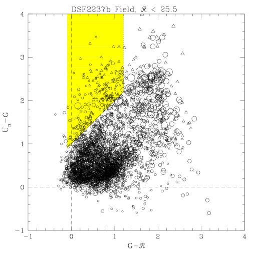
Figure 2: A two–color diagram typical of those used to identify Lyman break galaxy candidates for spectroscopic follow–up. The region of the color–color plane populated by Lyman break galaxies in the redshift range $2.6\lower 2.15277pt\hbox{$\;\buildrel<\over{\sim}\;$}z\lower 2.15277pt\hbox{$\;\buildrel<\over{\sim}\;$}3.4$ is shaded. This example includes 3300 objects in a field of size 9${}^{\prime}\mskip-4.7mu.\mskip 0.8mu$1 by 9${}^{\prime}\mskip-4.7mu.\mskip 0.8mu$1; a total of 140 of the objects to ${\cal R}=25.5$ satisfies the adopted color selection criteria, or about 4% of the total.

It is possible to make simple predictions of the spectral energy distributions of distant galaxies, (e.g., Steidel, Pettini, & Hamilton 1995) based on modeling the far–UV spectra of star forming galaxies, and including the effects of both Lyman continuum opacity of the galaxy interstellar medium and the known statistical effects of the intergalactic medium [see Madau 1995 for an in-depth discussion of the latter effect]. Based on such predictions, one can isolate a region of ”color-color space” in a diagram such as that shown in Figure 2, in which only galaxies at $z>2.6$ should be found. One would predict that a sample selected from that region would have a redshift distribution that is limited on the low–redshift side by the necessity of observing a significant ”break” across the Lyman limit in the fixed $U_{n}$ and $G$ passbands, and on the high redshift side by the $G-{\cal R}$ color, which becomes increasingly “reddened” by the blanketing from the Lyman alpha forest. Both these effects are rather easily modeled, and even before any confirming spectroscopy, one might predict that the redshift range for objects in the shaded region of Fig. 2 would be $2.7\lower 2.15277pt\hbox{$\;\buildrel<\over{\sim}\;$}z\lower 2.15277pt\hbox{$\;\buildrel<\over{\sim}\;$}3.5$. In a sense this use of colors is akin to the increasingly popular ”photometric redshift” method, but our real intention is not to measure redshifts with photometry, but to obtain something close to a a volume–limited (really, redshift–bounded) sample of galaxies where the culling process would be highly efficient. Quite honestly, even in our most optimistic times during several years of collecting photometric data (see, e.g., Steidel, Pettini, & Hamilton 1995) we would not have imagined how cleanly this this method could be implemented with ground-based photometry of very faint galaxies.

It was our first opportunity to use the Low Resolution Imaging Spectrograph (Oke et al. 1995) on the (then only) Keck telescope in September of 1995 that allowed us to convince ourselves and others that the method would really work (Steidel et al. 1996). It quickly became clear that it would be feasible to construct large samples of $z\sim 3$ galaxies with some concentrated effort; we thus began a project to obtain images in our $U_{n}G{\cal R}$ photometric system of relatively large regions of sky, from which Lyman break candidates could be selected and followed up spectroscopically on the W.M. Keck telescopes. The rationale for undertaking such a survey was that a large statistically homogeneous sample was bound to be useful for a general understanding of the nature of the high redshift star forming galaxy population, and it would almost certainly provide unprecedented information on the clustering properties of very early galaxies, which one might expect to provide a very sensitive cosmological test.

Figure 3: The histogram of spectroscopically confirmed Lyman break galaxies as of 1998 May. Note the well–defined sensitivity of the survey in redshift space, fairly well-characterized by a Gaussian centered at $z=3.0$ with a dispersion $\mathchar 28955\relax_{z}=0.25$.

2 The Lyman Break Galaxy Survey

The present goal of the LBG Survey is to cover 5-6 fields, each of size 150–250 square arc minutes, for a total sky coverage of about 0.3 square degrees. A typical survey field is 9${}^{\prime}~{}$ by 18${}^{\prime}~{}$  so that the transverse co-moving scale is $\sim 12h^{-1}\times 24h^{-1}$ Mpc for $\Omega_{m}=0.2$ open and $\Omega=0.3$ flat, and $\sim 8h^{-1}\times 16h^{-1}$ Mpc for $\Omega_{m}=1$; the effective survey depth is $\sim 400h^{-1}$ Mpc for the low–density models and $\sim 250h^{-1}$ Mpc for Einstein-de Sitter. Within the full survey area, there will be approximately 1500 objects satisfying the color criteria illustrated in Figure 2. The aim is to obtain confirming spectra for approximately 50% or more of the photometric sample in the primary survey fields. The redshift histogram of spectroscopically–confirmed objects at the time of this writing (May 1998) is shown in Figure 3. Of these, 437 redshifts have been obtained in what we now consider to be our primary survey fields. To a large extent, the “bottle–neck” in the progress of the survey is in obtaining the deep CCD images necessary for accurate photometric selection; these images require approximately 2 clear nights on a 4-meter class telescope per pointing, and most of our photometry has been obtained at the prime focus of the Palomar 200–inch telescope, which provides a field of only $\sim 9$${}^{\prime}~{}$ square. A clear night with LRIS on the Keck II telescope will typically yield 50-60 confirmed $z\sim 3$ galaxies, so that the entire survey could in principle be completed after a total of 15-20 nights (we are approximately 60% finished at this time).

Figure 3 shows that the peak of the sensitivity of the survey lies at $z=3.02$, with about 90% of the objects lying in the interval [2.7,3.4]. The survey is obviously incomplete on either side of the median redshift; to calculate the effective volume covered by the survey we assume that it is 100% complete at $z=3$ and that the true LBG density does not change significantly over the range of interest. To ${\cal R}=25.0$, the observed surface density of Lyman break galaxies satisfying the color criteria illustrated in Figure 2 is 1.0 per square arc minute, corresponding to co–moving space densities of $6.4\times 10^{-3}h^{3}$ Mpc^-1 ($\Omega_{m}=1)$ or $1.7\times 10^{-3}h^{3}$ Mpc^-3 for either $\Omega_{m}=0.2$ open or $\Omega_{m}=0.3$ flat. For an Einstein-de Sitter Universe, the space density integrated to ${\cal R}=25.0$ is roughly equivalent to the present–day space density of galaxies with $L>L^{\ast}$; the density is 4 times smaller than this for a universe with $\Omega_{m}\sim 0.2-0.3$. Thus, the sample of Lyman break galaxies represents relatively common objects, albeit objects at the bright end of the far-UV luminosity distribution, and in the absence of severe censoring by dust, these are the objects harboring the most vigorous star formation at $z\sim 3$.

Discussions of the far-UV luminosity function, the extinction corrections that are likely to apply to the LBG population (and therefore the corrected star formation rates), and the spectroscopic and morphological properties of the sample have been, or will soon be, presented elsewhere (e.g., Pettini et al. 1997, 1998; Dickinson 1998; Giavalisco 1998; Steidel et al. 1998b).

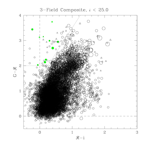
Figure 4: The upper panel shows an example of a color–color diagram that can be used to select galaxies in the range $3.9\lower 2.15277pt\hbox{$\;\buildrel<\over{\sim}\;$}z\lower 2.15277pt\hbox{$\;\buildrel<\over{\sim}\;$}4.5$ in a manner analogous to the $z\sim 3$ method. The filled symbols represent objects which have been confirmed spectroscopically in the expected redshift range. The lower panel shows example spectra; the first two clearly have very strong Lyman $\mathchar 28939\relax$ emission, whereas the third is much weaker (and unfortunately much more typical). Note the strong continuum break shortward of Lyman $\mathchar 28939\relax$ emission due to the onset of the Lyman $\mathchar 28939\relax$ forest.

An obvious extension of the current Lyman break selection technique is to move the method to higher redshifts using a different filter system. It has been straightforward to obtain data in one additional passband, $i$[8100/1200], in our survey fields, so that one can search for objects exhibiting “breaks” in the $G$ band rather than the $U_{n}$ band. Models similar to those used for defining the initial color cuts for $z\sim 3$ galaxies can be used to predict that, for the color criteria defined in Figure 4a, the range of redshifts should be $3.9\lower 2.15277pt\hbox{$\;\buildrel<\over{\sim}\;$}z\lower 2.15277pt\hbox{$\;\buildrel<\over{\sim}\;$}4.5$, for an expected median redshift of $z\sim 4.2$. Our spectroscopic sample in this redshift range is still relatively small (example spectra of $z>4$ Lyman break galaxies are shown in Figure 4b), but not surprisingly the “predictions” are largely borne out. What is clear from our experimentation with the $z\sim 4.2$ samples is that a large survey aimed at establishing the large-scale distribution at this higher redshift interval would be much more difficult that at $z\sim 3$. The reason for this is almost completely practical— at $z\sim 3$, all of the spectroscopic features useful for redshift identification fall comfortably in the 4500–6500 Å range, where the sky background is very dark, the instrumental throughput is at a maximum, and there is no fringing of the CCD which severely compromises one’s ability to do precision sky subtraction at longer wavelengths. At $z\sim 4.2$, the same features have moved into the $6300-8000$ Å range, where the sky is much brighter and sky subtraction much more subject to systematic difficulties produced by fringing and the “forest” of OH emission lines in the sky. As a result, the efficiency with which one can go from photometric candidates to spectroscopic confirmations is down by a factor of $\sim 5$, and it becomes especially difficult to confirm objects without strong Lyman $\mathchar 28939\relax$ emission lines. For this reason, we do not intend any major galaxy survey at $z\sim 4.2$, but our aim instead is to establish the redshift selection function in order to make a statistically significant differential comparison of the space density of star-forming galaxies at $z\sim 4.2$ relative to those at $z\sim 3$, as we regard it as very important to check the result implied in the Hubble Deep Field (Madau et al. 1996) that the space density of Lyman break galaxies is significantly lower at $z\sim 4$ than at $z\sim 3$.

In parallel with the large spectroscopic survey, we are also pursuing programs involving near–IR imaging of sub-samples using Keck/NIRC, observations in the sub–mm continuum of the most apparently reddened examples of $z\sim 3$ LBGs using SCUBA on the JCMT, near–IR spectroscopy in order to obtain line widths and fluxes of rest–frame optical nebular lines using UKIRT+CGS4 (Pettini et al. 1998), and higher-dispersion optical spectroscopy of selected bright examples using LRIS on Keck. Since most of these investigations are related more to the astrophysics of the individual galaxies, rather than their large-scale distribution, we will not discuss the results further in the present summary.

3 Large Scale Structure at $z\sim 3$

It was quite obvious (even at the telescope) during our first observing runs spent collecting significant numbers of Lyman break galaxy spectra over relatively large fields that the redshifts were far from randomly distributed throughout the survey volume. Strong redshift–space clustering is certainly not a new phenomenon for redshift surveys having “pencil–beam” geometries (e.g., Broadhurst et al. 1990, Cohen et al. 1996); nevertheless, it was somewhat surprising to encounter significant “spikes” in the redshift distribution at $z\sim 3$, where naively one might expect clustering to be significantly weaker than at $z<1$ under any structure formation scenario that involves gravitational instability.

The first field for which a significant number of redshifts was obtained, SSA22 (see the top left panel of Figure 5), yielded a structure on a scale of $\sim 10$ Mpc that would be extremely rare for any cosmology (even for $\Omega_{m}=0.2$) if galaxy number density fluctuations were an unbiased tracer of matter fluctuations and if one adopted “cluster normalization” for the value of $\mathchar 28955\relax_{8}$ (e.g., Eke, Cole, and Frenk 1996). To have a significant probability of being found, a peak with the observed over-density on the observed scale requires significant bias of the galaxy fluctuations as compared to underlying mass fluctuations (Steidel et al. 1998a). With a bias parameter on $\sim 10$ Mpc scales defined in the usual way, $b\equiv\mathchar 28942\relax_{\rm gal}/\mathchar 28942\relax_{\rm mass}$, and assuming that such a peak would be found in every survey field, a “high peak” analysis would require that $b\lower 2.15277pt\hbox{$\;\buildrel>\over{\sim}\;$}6$ for an Einstein-de Sitter universe; the corresponding numbers would be $b\lower 2.15277pt\hbox{$\;\buildrel>\over{\sim}\;$}2$ for $\Omega_{m}=0.2$ (open) and $b\lower 2.15277pt\hbox{$\;\buildrel>\over{\sim}\;$}4$ for $\Omega_{m}=0.3$ (flat). Our first reaction was that the very high galaxy bias required in the universe with $\Omega_{m}=1$ was too high, and that this favored a low–density universe. However, it turned out that such large values of the bias emerge naturally for rare dark matter halos that are just collapsing at the epoch corresponding to $z\sim 3$, within the context of CDM–like models for both N-body simulations (Jing & Suto 1998; Bagla 1998; Wechsler et al. 1998; Governato et al. 1998) and for analytic variations of Press-Schechter theory (Press & Schechter 1974; Mo & Fukugita 1996; Mo & White 1996; Baugh et al. 1998). It was also interesting, as we had remarked, that if a similar large peak were found in each survey field, they would have just about the right space density to match that of present–day X-ray clusters, suggesting the possibility that the “spike” could be a proto–cluster viewed prior to collapse and virialization (there was no evidence for central concentration of the galaxies within the “spike” on the plane of the sky). This interpretation is indeed supported by the simulations (Wechsler et al. 1998, Governato et al. 1998). In any case, despite the frustrating result that strong clustering was expected for the most massive virialized halos at $z\sim 3$ in any hierarchical model, it was clear that the general paradigm of “biased” galaxy formation (Kaiser 1984; Bardeen et al. 1986; Cole & Kaiser 1989) was strongly supported. Nevertheless, the numbers were quite uncertain based on a single high peak in a single survey field, and it was clearly essential to obtain more data so that the galaxy fluctuations could be better–characterized.

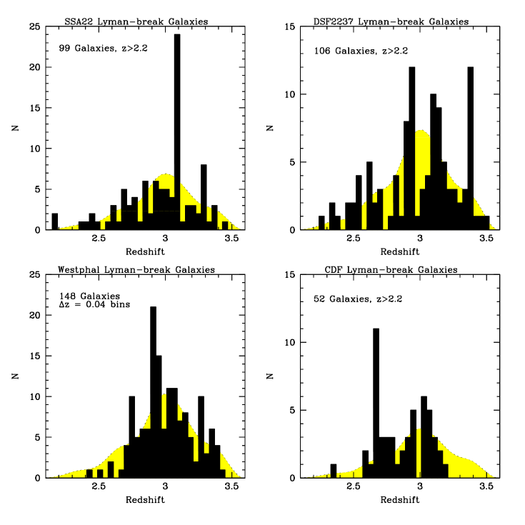
Figure 5: Redshift histograms (to date) in 4 of our survey fields to date. The transverse size of the surveyed fields varies: 8${}^{\prime}\mskip-4.7mu.\mskip 0.8mu$7 by 8${}^{\prime}\mskip-4.7mu.\mskip 0.8mu$7 (CDF), 9${}^{\prime}~{}$ by 18${}^{\prime}~{}$ (DSF2237, SSA22), 15${}^{\prime}\mskip-4.7mu.\mskip 0.8mu$0 by 15${}^{\prime}\mskip-4.7mu.\mskip 0.8mu$0 (Westphal). In each case, the light histogram indicates the empirical redshift selection function imposed by the photometric selection, normalized to the same number of objects as observed. Note the prominent redshift “spikes” present in each field.

Figure 5 contains redshift histograms from 4 of our survey fields, showing that large fluctuations are indeed generic. To make this more quantitative, we have recently analyzed the counts-in-cells fluctuations of LBGs within six 9${}^{\prime}~{}$ by 9${}^{\prime}~{}$ fields in which the spectroscopy is reasonably complete (Adelberger et al. 1998). This type of analysis, which takes into account not just the highest peak, but general fluctuations on a fixed co-comoving scale, should provide a much more robust estimate of the effective bias of the LBGs. The cells were cubes of side length defined by the transverse size of the field, or $\sim 8h^{-1}$ Mpc for $\Omega_{m}=1$ and $\sim 12h^{-1}$ Mpc for $\Omega_{m}=0.2$ open and $\Omega_{m}=0.3$ flat models. After correcting for shot noise, we found that $\mathchar 28955\relax_{\rm gal}=1.1\pm 0.2$, implying that $b\equiv\mathchar 28955\relax_{\rm gal}/\mathchar 28955\relax_{\rm mass}$ is $6\pm 1$, $1.9\pm 0.4$, and $4.0\pm 0.7$ for $\Omega_{m}=1$, $\Omega_{m}=0.2$ open, and $\Omega_{m}=0.3$ flat. These numbers are in very good agreement with our initial estimate from a single high peak in the first field observed. If these inferred bias values are used to estimate the more familiar galaxy–galaxy correlation length $r_{0}$, then for a power law slope $\mathchar 28941\relax=-1.8$ for the correlation function, the co-moving correlation length would be $r_{0}=4h^{-1}$, $6h^{-1}$, and $5h^{-1}$ Mpc for $\Omega_{m}=1$, $\Omega_{m}=0.2$ open, and $\Omega_{m}=0.3$ flat, respectively. Note that these values are roughly the same as the correlation length for galaxies today, indicating the very strong bias that must be present relative to the mass distribution in any reasonable gravitational instability scenario (cf. Baugh et al. 1998, who predicted similar correlation lengths for Lyman break galaxies using their semi-analytic galaxy formation model). The published correlation lengths for intermediate redshift galaxy samples are significantly smaller (cf. Le Fèvre et al. 1996, Carlberg et al. 1997), illustrating that the correlation strength of galaxy samples is almost certainly strongly dependent on redshift and sample selection method in ways that are not normally accounted for in simple models (see Giavalisco et al. 1998a).

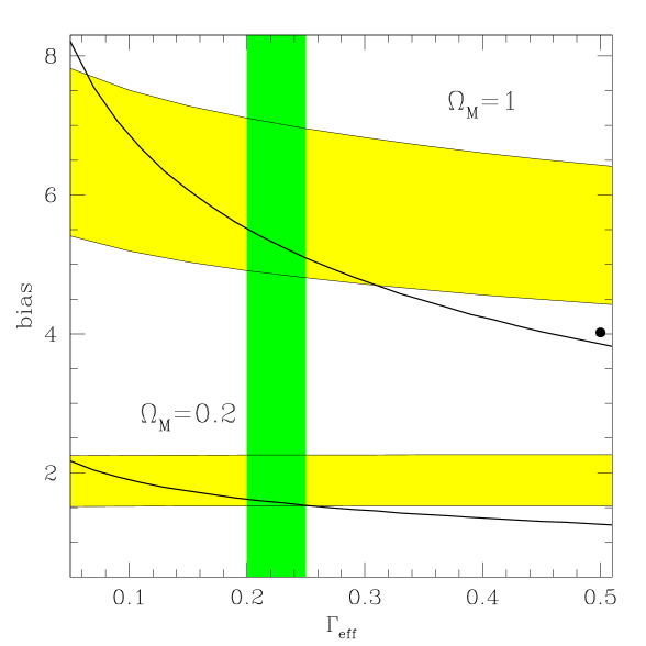
Figure 6: A plot comparing the abundance and clustering properties of observed galaxies and theoretical dark matter halos, from Adelberger et al. 1998. The horizontal shaded regions show the inferred bias (on $\sim 10$ Mpc scales) for observed LBGs, versus a parameterization of the shape of the mass fluctuation power spectrum. Analyses of present–day large scale structure suggest a value of $\Gamma$ in the range $0.2\lower 2.15277pt\hbox{$\;\buildrel<\over{\sim}\;$}\Gamma\lower 2.15277pt\hbox{$\;\buildrel<\over{\sim}\;$}0.25$ (e.g., Peacock & Dodds 1994), shown with the vertical shaded region. (In this context, $\Gamma$ can be thought of as an indicator of the relative power on galaxy [$\sim 1$ Mpc] and cluster [$\sim 10$ Mpc] scales). The solid curves show the predicted bias of halos having the same abundance as the observed Lyman break galaxies. Note the good agreement between the predictions and the observations if $\Gamma\sim 0.2$, and that standard CDM (the dark point) is discrepant by about 2 $\mathchar 28955\relax$.

Once a reasonable estimate of the LBG bias is available, it is possible to make more detailed comparisons to dark matter models. In particular, a successful model should be able to produce simultaneously both the observed strong clustering of the LBGs, and the right number density of halos exhibiting that strong clustering. The number density reflects the level of power on galaxy ($\sim 1$ Mpc) scales, while the strong clustering we observe (e.g., in Figure 5) reflects power on $\sim 10$ Mpc scales; a model will be able to match both observational constraints simultaneously only if it has the right ratio of power on these two scales. This is illustrated in Figure 6, where the ratio of power on these scales is parameterized in the usual way with the power spectrum “shape parameter”, $\Gamma$. Higher values of $\Gamma$ correspond to larger ratios of small to large scale power, and (as explained in Adelberger et al. 1998) to weaker clustering for objects of fixed abundance. $\Gamma\lower 2.15277pt\hbox{$\;\buildrel<\over{\sim}\;$}0.2$ is apparently required to reconcile the dark matter model and the LBG observations; similar values are implied by observations of galaxy clustering on scales $>10$ Mpc in the local universe. Both the theoretical and observational estimates of $b$ in Figure 6 are based on the same cluster normalization for $\mathchar 28955\relax_{8}$, so that changing the normalization will move the theoretical curve and the empirical estimates of $b$ in much the same way (this explains why the shape of the curves in Figure 6 are very similar for very different values of $\Omega_{m}$). The most important point to glean from Figure 6 is that one can match both the abundance and the clustering properties (parameterized here by the value of $b$ on $\sim 10$ Mpc scales) of dark matter halos and the observed galaxies using a simple model, provided that the shape of the power spectrum is in the same range implied by local estimates of large scale structure.

An additional test of a generic hierarchical model would be that more abundant objects must be less strongly clustered (i.e., less massive halos must exhibit smaller values of $b$). Figure 7 shows the predictions of $b$ versus abundance for a model having $\Gamma=0.2$. Again, there is no fitting involved here, and it can be seen that in fact the much more abundant, much fainter LBGs from the Hubble Deep Field sample are in fact much less strongly clustered, entirely consistent with the predictions of the simple model (see Giavalisco et al. 1998b for a complete description of the models and of the HDF sample). Also of note is that models with low $\Omega_{m}$ and Einstein-de Sitter models are equally capable of matching the observations, given a spectral shape fixed at $\Gamma=0.2$; in both models, the relatively rare peaks in the density field are expected to be strongly clustered (although the bias relative to the overall mass distribution is very different) and to have roughly the same dependence on halo number density. A very large difference, however, exists in the predicted mass scales for the most strongly biased dark matter halos. In the $\Omega=0.2$ model, the characteristic mass of halos having the abundance (and clustering properties) of the spectroscopic LBG sample is $\sim 3\times 10^{12}$ M${}_{\mbox{$\odot$}}$, whereas the predicted mass of the same objects in the $\Omega_{m}=1$ model is only $1.3\times 10^{11}$, a difference of more than a factor of 20! While dynamical mass estimates of these high redshift galaxies are extremely challenging (see Pettini et al. 1998), the differences are so large that it may be quite plausible to discriminate observationally between the two cosmologies.

Figure 7: The predicted bias as a function of halo abundance for a dark matter model with $\Gamma=0.2$, together with data from 3 different samples of LBGs. The point marked ”S” is based on the spectroscopic sample discussed above; the point marked ”P” is from a larger and slightly fainter photometric sample for which the clustering properties were estimated using the observed angular correlation function together with the observed redshift selection function (Giavalisco et al. 1998a). The point marked ”HDF” comes from a $w(\mathchar 28946\relax)$ analysis of F300W ”dropouts” to $F606W=27$ in the Hubble deep field; the error bars reflect the uncertainties due to the fact that the redshift selection function for the HDF color selection criteria are not precisely known. Note that no ”fitting” of the model curve has been imposed.

4 What Does It All Mean?

The data are obviously just reaching the level where quantitative analyses are possible, and there is no doubt that the observational situation can be improved dramatically on a short timescale. However, based on what must be considered preliminary analysis of the current data, it is already possible to list some broad conclusions that are unlikely to change substantially.

First, the clustering properties of Lyman break galaxies, which are selected on the basis of their rest–frame far-UV flux, indicate that they are associated with relatively rare, massive dark matter halos. This is true independent of the matter density; however, for a power spectrum shape that obeys local constraints ($\Gamma\sim 0.2$), the mass scale associated with the most luminous LBGs is strongly $\Omega_{m}$–dependent. For low–density models, the halo mass scale is $\sim 10^{12}$ M${}_{\mbox{$\odot$}}$, already similar to massive galaxies at the present epoch. The strong clustering of massive halos is expected for standard hierarchical models in which the fluctuations are Gaussian, and thus the LBGs are apparently tracing regions of enhanced mass density at early epochs. In the context of models of hierarchical growth of structure, this means by and large that the descendents of LBGs would be found as parts of much larger virialized structures in the universe today (e.g., Steidel et al. 1998; Governato et al. 1998; Wechsler et al. 1998). The strongest peaks in the distribution of LBGs at high redshift are likely to be the progenitors of rich clusters of galaxies, which one is apparently seeing prior to collapse and virialization. Regardless of the details of one’s interpretation, the “paradigm” that galaxies form at the (biased) high peaks in the dark matter distribution is very strongly supported by the data.

The statistics are now good enough that an attempt to reconcile the abundance and clustering properties of LBGs with models is justified. Quite remarkably (in our opinion), there is amazingly good agreement between the predictions of a simple dark matter model having the power spectrum shape constrained by local large scale structure, and the observed galaxies. As discussed in Adelberger et al. 1998, this agreement depends on a very tight relationship between dark matter halo mass and far–UV luminosity, as this is implicit in matching observed galaxies to dark matter halo abundances. If it were the case that star formation were a highly stochastic process, in which halos differing substantially in mass could produce the same star formation rate, it would “dilute” the clustering properties of a sample selected by UV luminosity so that it would not result in clustering as strong as observed. Further, it is difficult to reconcile the models and the data unless there is essentially a one-to–one correspondence between observable galaxies and dark matter halos (if we were observing only a small fraction of the strongly–clustered massive halos, then this would present a problem for any hierarchical model). This, incidentally, argues against a large population of star forming galaxies completely obscured by dust, and also against models in which the LBGs are undergoing brief bursts of star formation that “light up” only a small fraction of the halos at a time. The bottom line that seems to make everything pleasingly consistent (although not necessarily correct, of course!) is that the most “visible” galaxies reside within the most massive dark matter halos, and that generally speaking the star formation rate is proportional to the halo mass. We believe that this kind of result provides strong empirical justification for the general application of semi-analytic models which treat star formation as a function of the parent dark matter halo properties using physically–motivated “recipes” (Baugh et al. 1998, Kauffman, Nusser, & Steinmetz 1998). It is possible that further direct comparison of the models to the observations could provide a means of fine-tuning the star formation prescriptions.

Regardless of the degree to which one is willing to believe that the observations and theory are now pointing in the same direction, it is certain to be the case that considerable progress in our understanding of the very-much-intertwined questions of galaxy formation and the development of large scale structure will be made in the immediate future. While at some level it is a bit of a disappointment that galaxy clustering at high redshift is not telling us unambiguously about the background cosmology, it certainly is the case that the observations can provide important tests of our collective ideas about how, where, and when galaxies form relative to the dark matter distribution. It may well be that the relative simplicity in interpretation allowed by observations at very high redshift will more than make up for the difficulty of obtaining the data.

5 Acknowledgments

Much of the work described would not have been possible without the generous gift from the W. M. Keck Foundation that allowed the construction of the Keck Observatory, and the many people involved in building and supporting the telescopes and the Low Resolution Imaging Spectrograph. This work has been financially supported by the US National Science foundation (CS, KA, MK) and by grant HF-01071.01-94A from the Space Telescope Science Institute (MG).

References

- 1 Adelberger, K. L., Steidel, C. C., Giavalisco, M., Dickinson, M., Pettini, M., & Kellogg, M. 1998, ApJ, in press.
- 2 Bagla, J. S. 1998, MNRAS, in press.
- 3 Baugh, C.M., Cole, S., Frenk, C.S., & Lacey, C.G. 1998, ApJ, 498, 504
- 4 Bardeen, J. M., Bond, J. R., Kaiser, N., & Szalay, A.S. 1986, ApJ, 304, 15
- 5 Broadhurst, T., Ellis, R. S., Koo, D., & Szalay, A. 1990, Nature, 343, 726
- 6 Carlberg, R.G., Cowie, L. L., Songaila, A., & Hu, E. M. 1997, ApJ, 484, 538
- 7 Cohen, J.G., Hogg, D.W., Pahre, M.A., & Blandford, R. D. 1996, ApJ, 462, L9
- 8 Cole, S. & Kaiser, N. 1989, MNRAS, 237, 1127
- 9 Cowie, L. L., Songaila, A., Hu, E. M., & Cohen, J. G. 1996, AJ, 1112, 839
- 10 Dickinson, M. 1998, in The Hubble Deep Field, ed. M. Livio, M. Fall, & P. Madau, (Cambridge: CUP), in press
- 11 Eke, V. R., Cole, S., & Frenk, C. S. 1996, MNRAS, 282, 263
- 12 Giavalisco, M. 1998, in The Hubble Deep Field, ed. M. Livio, M. Fall, & P. Madau, (Cambridge: CUP), in press
- 13 Giavalisco, M., Steidel, C. C., Adelberger, K. L., Dickinson, M. E., Pettini, M., & Kellogg, M. 1998a, ApJ, in press
- 14 Giavalisco, M. et al. 1998b, in preparation
- 15 Governato, F., Baugh, C. M., Frenk, C. S., Cole, S., Lacey, C. G., Quinn, T., & Stadel, J. 1998, Nature, 392, 359
- 16 Jing, Y. P. & Suto, Y. 1998, ApJL, submitted
- 17 Kaiser, N. 1984, ApJL, 284, L9
- 18 Kauffmann, G., Nusser, A., & Steinmetz, M. 1997, MNRAS, 286, 795
- 19 Le Fèvre, O., Hudon, D., Lilly, S. J., Crampton, D., Hammer, F., & Tresse, L. 1996, ApJ, 461, 534
- 20 Madau, P. 1995, ApJ, 441, 18
- 21 Madau, P., Ferguson, H.C., Dickinson, M., Giavalisco, M., Steidel, C.C., & Fruchter, A. 1996, MNRAS, 283, 1388
- 22 Mo, H. J., & Fukugita 1996, ApJ, 467, L9
- 23 Mo, H. J., & White, S. D. M., 1996, MNRAS, 282, 347
- 24 Oke, J. B. et al. 1995, PASP 107, 3750
- 25 Peacock, J. A., & Dodds, S. J. 1994, MNRAS, 267, 1020
- 26 Pettini, M., Kellogg, M., Steidel, C. C., Dickinson, M., Adelberger, K. L., & Giavalisco, M. 1998, ApJ, in press.
- 27 Press, W. H. & Schechter, P. 1974, ApJ, 187, 425
- 28 Steidel, C. C., Adelberger, K. L., Dickinson, M., Giavalisco, M., Pettini, M. & Kellogg, M. 1998a, ApJ, 492, 428
- 29 Steidel, C. C., Adelberger, K. L., Dickinson, M., Giavalisco, M., Pettini, M., & Kellogg, M. 1998b, in The Young Universe, eds. A. Fontana & S. D’Odorico (San Francisco: ASP), in press.
- 30 Steidel, C. C., Giavalisco, M., Pettini, M., Dickinson, M., & Adelberger, K. L. 1996, ApJ, 462, L17
- 31 Steidel, C. C., Pettini, M., & Hamilton, D. 1995, AJ, 110, 2519
- 32 Steidel, C. C., & Hamilton D. 1992, AJ, 104, 941
- 33 Steidel, C. C., & Hamilton, D. 1993, AJ, 105, 2017
- 34 Wechsler, R. H., Gross, M. A. K., Primack, J. R., Blumenthal, G. R. & Dekel, A. 1998, ApJ, submitted
- 35 White, S. D. M. & Rees, M. J. 1978, MNRAS, 183, 341