A Study of Nine High-Redshift Clusters of Galaxies:
II. Photometry, Spectra, and Ages of Clusters 0023+0423 and 1604+4304

Abstract

We present an extensive photometric and spectroscopic study of two high-redshift clusters of galaxies based on data obtained from the Keck 10m telescopes and the Hubble Space Telescope. The clusters CL0023+0423 ($z=0.84$) and CL1604+4304 ($z=0.90$) are part of a multi-wavelength program to study nine candidate clusters at $z\mathrel{\hbox{\raise 2.15277pt\hbox{$>$}\hbox to0.0pt{\hss\lower 2.15277pt\hbox{$\sim$}}}}0.6$ (Oke, Postman & Lubin 1998). Based on these observations, we study in detail both the field and cluster populations. From the confirmed cluster members, we find that CL0023+0423 actually consists of two components separated by $\sim$2900 km s^-1. A kinematic analysis indicates that the two components are a poor cluster with $\sim$3 $\times 10^{14}$ M_⊙ and a less massive group with $\sim$10¹³ M_⊙. CL1604+4304 is a centrally concentrated, rich cluster at $z=0.8967$ with a velocity dispersion of 1226 km s^-1 and a mass of $\sim$3 $\times 10^{15}$ M_⊙.

A large percentage of the cluster members show high levels of star formation activity. Approximately 57% and 50% of the galaxies are active in CL0023+0423 and CL1604+4304, respectively. These numbers are significantly larger than those found in intermediate-redshift clusters (Balogh et al. 1997). We also observe many old, red galaxies. Found mainly in CL1604+4304, they have spectra consistent with passive stellar evolution, typical of the populations of early-type galaxies in low and intermediate-redshift clusters. We have calculated their ages by comparing their spectral energy distributions to standard Bruzual & Charlot (1995) evolutionary models. We find that their colors are consistent with models having an exponentially decreasing star formation rate with a time constant of 0.6 Gyr. We also observe a significant luminosity brightening in our brightest cluster galaxies. Compared to brightest cluster galaxies at $z\sim 0.1$, we find a luminosity increase of $\sim 1$ mag in the rest $M_{B}$ and $\sim 0.8$ mag in the rest $M_{V}$.

In the field, we find that $\sim 76\%$ of the galaxies with $z>0.4$ show emission line activity. These numbers are consistent with previous studies (e.g. Hammer et al. 1997). We find that an exponentially decaying star formation rate is required to produce the observed amount of star formation for the majority of the galaxies in our sample. A time constant of $\tau=0.6$ Gyr appears to be optimal. We also detect several interesting galaxies at $z>1$. Two of these galaxies are extremely luminous with strong MgII$\lambda$2800 absorption and FeII resonance line absorption. These lines are so strong that we conclude that they must be generated within the atmospheres of a large population of young, hot stars.

Accepted for publication in the Astronomical Journal

1 Introduction

The study of cluster galaxies at moderate look-back times of $50-70$% of the cosmic age ($0.7\mathrel{\hbox{\raise 2.15277pt\hbox{$<$}\hbox to0.0pt{\hss\lower 2.15277pt\hbox{$\sim$}}}}z\mathrel{\hbox{\raise 2.15277pt\hbox{$<$}\hbox to0.0pt{\hss\lower 2.15277pt\hbox{$\sim$}}}}1.5$) can provide important constraints on the nature and duration of the processes which have yielded the current epoch distribution of galaxy properties. This intermediate redshift range is likely to be a period where clusters are undergoing (or have recently completed) virialization and where many galaxies are only 1 or 2 Gyr past the peak in the cosmic star formation history (Madau, Pozzetti & Dickinson 1998). From a practical point of view, it is a regime which has only recently become readily accessible, both photometrically and spectroscopically, from space and ground-based optical and near-IR telescopes. In the redshift range from $z=0.3$ to $0.6$ there have been numerous photometric and/or spectroscopic studies of both optically and X-ray selected clusters (e.g. Koo (1981); Couch et al. (1983); Ellis et al. (1985); Couch, Shanks & Pence (1985); Couch & Sharples (1987); Couch et al. (1991); Fabricant, McClintock & Bautz (1991); Henry et al. (1992); Dressler & Gunn (1992); Oke, Gunn & Hoessel (1996)). Galaxies in these systems can be studied easily down to 5% of the characteristic luminosity and contamination by interlopers is not a significant problem.

A growing number of clusters with $z\leq 0.5$ have been extremely well-studied. With spectra of hundreds of cluster members, detailed modeling of the infall patterns and intracluster chemical composition gradients is now available (Abraham et al. (1996); Ellingson et al. (1997)). The above studies indicate that the cores of rich clusters are typically dominated by a population of luminous early-type, red galaxies which produce a remarkably narrow ridge (or “red locus”) in the color-magnitude (CM) relation. At $z\mathrel{\hbox{\raise 2.15277pt\hbox{$<$}\hbox to0.0pt{\hss\lower 2.15277pt\hbox{$\sim$}}}}0.4$ both the mean color and the CM relation are consistent with those of present-day ellipticals (e.g. Aragón-Salamanca et al. 1991; Dressler & Gunn 1992; Stanford, Eisenhardt & Dickinson 1994,1997). The bulk of these galaxies have spectra which show no obvious signs of current or recent star formation. However, there is a non-negligible fraction which show post-starburst spectra with strong Balmer lines in absorption (e.g. Gunn & Dressler 1988; Dressler & Gunn 1992; Poggianti 1997). In conjunction with this population is a fraction of blue cluster members which is increasing with redshift, a phenomenon known as the Butcher-Oemler effect (Butcher & Oemler 1984). Most of these galaxies appear as normal spirals or have peculiar morphologies (Dressler et al. 1994; Couch et al. 1994; Oemler, Dressler & Butcher 1997). A large fraction of this blue, spiral population exhibits exceptionally strong Balmer lines and/or [OII] emission which indicates that a significant fraction of the cluster members have recently undergone or are currently undergoing a high level of star formation activity (e.g. Lavery & Henry 1988; Gunn & Dressler 1998; Lavery, Pierce & McClure 1992; Dressler et al. 1994; Poggianti 1997).

Complimenting the ground-based work are several Hubble Space Telescope (HST) programs to quantify the morphology of galaxies in these clusters (e.g. Couch et al. (1994); Dressler et al. (1994); Smail et al. (1997); Oemler, Dressler & Butcher (1997); Ellis et al. (1997)). HST enables morphological classifications which can be made on scales of $\sim 1~{}{\rm kpc}$, thus providing a direct comparison to ground-based classifications of nearby galaxies. In addition to relating the photometric and spectral characteristics of a galaxy to its morphology, the HST studies can be used to examine the overall morphological distribution in these clusters. This work may indicate that the morphological composition of clusters is evolving with redshift (Dressler et al. 1997; Oemler, Dressler & Butcher 1997), though these results are not yet certain (e.g. Stanford, Eisenhardt & Dickinson 1997; Lubin et al. 1998). These evolutionary changes are also apparently reflected in the evolution of the morphology–density relation (Dressler (1980); Postman & Geller (1984)). This relation in intermediate-redshift clusters which are centrally-concentrated and compact is qualitatively similar to that in the local universe; however, unlike present-day clusters, the relation is non-existent in the loose, open clusters (Dressler et al. 1997).

Studies of clusters of galaxies with redshifts greater than $z=0.6$ are substantially more difficult because (1) the galaxies are approaching the sensitivity limits of optical spectrographs on 4m class telescopes, (2) the interloper contamination becomes substantial, and (3) the well understood rest wavelength region redward of 4000Å moves into the near infrared. Despite these difficulties, several studies of high-redshift clusters have been made. These studies indicate that the Butcher-Oemler effect continues to strengthen up to $z=0.9$ (Aragón-Salamanca et al. 1993; Rakos & Schombert 1995; Lubin 1996). In addition, the red envelope of the early-type cluster population moves bluewards with redshift. At $z\sim 0.9$ there are few galaxies with colors as red as present-day ellipticals (Aragón-Salamanca et al. 1993; Rakos & Schombert 1995; Oke, Gunn & Hoessel 1996; Lubin 1996; Ellis et al. 1997; Stanford, Eisenhardt & Dickinson 1995,1997). This color evolution is consistent with passive evolution of an old stellar population formed at an early cosmic age. The amount of color evolution is similar from cluster to cluster at a given redshift and is independent of the cluster richness or X-ray luminosity. These results indicate that the history of early-type galaxies may be insensitive to environment; that is, these galaxies appear to be coeval with a common star formation history (Bower et al. 1992a,b; Aragón-Salamanca et al. 1993; Dickinson 1995; Stanford, Eisenhardt & Dickinson 1995,1997; Ellis et al. 1997).

There have also been many studies of high-redshift field galaxies. Hamilton (1985) obtained spectra of 33 very red, field galaxies in the redshift range of $z=0.2$ to $z=0.8$. He found that the 4000 Å break changed by less than 7% over the observed $z$ range. Songaila et al. (1994) obtained $BVK$ photometry and spectra of a nearly complete sample of 298 galaxies. The redshifts are nearly all at $z<1.0$. They find no $K$–band luminosity evolution. From measurements of emission-line strengths and the 4000 Å break, they infer that galaxies are undergoing significantly more star formation at $z=1$ than at the present epoch. The Canada-France-Redshift-Survey (CFRS) group has used CFHT to carry out a very extensive spectroscopic survey out to redshifts of 1.3 (Lilly et al. (1995), Hammer et al. (1997)). They find that the fraction of galaxies with significant emission lines (EW of [OII] $>15$ Å) increases from about 13% locally to over 50% at $z>0.5$. The fraction of luminous, quiescent galaxies (no significent [OII] emission) decreases with redshift from 53% at $z=0.3$ to 23% for $z>0.5$. They also find evidence that the metal abundance is lower in emission-line galaxies at high redshifts than locally. In addition, Cohen et al. (1996a,b) have obtained spectra of high redshift galaxies in the fields of both the Hubble Medium Deep Survey and the Hubble Deep Field survey. They find that the redshifts are highly clumped; the velocity dispersion in these clumps are similar to those found in local groups of galaxies. Further supporting this observational evidence of strong velocity structure at high redshift, Koo et al. (1996) carried out photometry and spectroscopy of 35 galaxies with redshifts of 0.3 to 1.6. They found that half of the redshifts in their sample are actually in two structures at $z=0.81$ and $z=1.0$.

Because studies of both field and cluster galaxies indicate that the high-redshift universe is a place of substantial evolution, we have undertaken an extensive program to study nine candidate clusters of galaxies at $z\mathrel{\hbox{\raise 2.15277pt\hbox{$>$}\hbox to0.0pt{\hss\lower 2.15277pt\hbox{$\sim$}}}}0.6$ (Oke, Postman & Lubin 1998; hereafter Paper I). With the commissioning of the Keck 10 meter telescopes, this detailed survey is now possible. The first paper in the series describes the sample selection, data acquisition, and data reduction procedures of the survey (Paper I). In this paper, we present our analysis and interpretation of the spectra and photometry for the first two clusters to be completed, CL0023+0423 ($z=0.84$) and CL1604+4304 ($z=0.90$). In the third paper of this series (Lubin et al. 1998; hereafter Paper III), the HST observations and the resulting morphological composition of these two clusters are described.

2 Keck LRIS Observations

Broad-band $BVRI$ and low-resolution spectroscopic data were obtained for CL0023+0423 and CL1604+4304 using the Low Resolution Imaging Spectrograph (LRIS; Oke et al. 1995) at the W.M. Keck Observatory. The details of these observations are presented in Paper I. We present here only a brief summary of the relevant information. The LRIS imaging for CL0023+0423 was obtained under photometric conditions. Spectra were taken using six different masks. The weather was photometric for four of the slit masks but marginal for the other two. Consequently, a second observation for one of the masks was obtained. In the case of CL1604+4304 the weather was photometric for all the broad-band imaging and for the six slit mask observations. Figures 1 and 2 show composite $BVR$ images for these two clusters.

For the spectrophotometric observations a list was made of all objects in a $600\times 2000$ pixel area ($2.15\times 7.16$ arcminutes) down to a Johnson-Cousins R magnitude of 23.3. The very few objects brighter than $R=18.3$ were excluded from the list, as well as those objects which have $y$ coordinates too close to the two selected set stars to allow spectra to be obtained. This produced a sample of 167 objects for CL0023+0423 and 168 for CL1604+4304. A summary of the spectroscopic observations is provided here in Table 1. The numbered rows give in order (1) the number of objects in the sampled region of sky, (2) the number of these objects which did not have a slit positioned on them and, hence, no spectrum was obtained, (3) the number of objects which have spectra but for which no redshift was determined, (4) the number of stars and very low $z$ galaxies ($z\leq 0.01$), (5) the number of quasars found, (6) the remaining number of objects which have redshifts, and (7) the number of these which have emission lines.

2.1 Spectroscopy

2.1.1 Redshifts

The spectra cover the wavelength range of $\sim$4500 Å to 9500 Å (see Paper I). The redshift determination is described fully in Paper I. The full lists of candidates for which spectra were attempted are given in Table 2 for the CL0023+0423 field and Table 3 for the CL1604+4304 field. Spectra were obtained for approximately 80% of the candidate objects; redshifts were determined for 90% of those. At redshifts above $z\sim 0.4-0.5$, the $[{\rm OII}]\lambda 3727$ line is observed. In the CL0023+0423 and CL1604+4304 fields, the fraction of objects with spectra that have emission lines is 89% and 79%, respectively. Assuming that the objects for which redshifts were not obtained do not have emission lines, the fraction of faint galaxies with emission lines is more like 78% and 70%, respectively, for the two cluster fields.

The resulting redshifts and qualities of the redshifts are given in columns 6 and 7 of Tables 2 and 3. The number 9.0000 in the tables means that a spectrum was obtained but no redshift could be derived. Stars and galaxies with redshifts less than 0.01 are listed as $z=0.0000$. The quality of a redshift is specified by a number from 1 to 4 which roughly corresponds to the number of features identified. A quality of 4 means that the redshift is certain. Quality 3 indicates that the redshift is almost certainly correct. Quality 2 means the redshift is probably correct while quality 1, which corresponds to only 1 emission line being seen , means the redshift is possible. In the cases where a single emission line can only be identified with [OII] the quality is set to 2. The distributions of spectroscopic targets on the sky and in redshift for the two cluster fields are shown in Figures 3 and 4. The results are summarized in Table 4 which lists the number of objects and the mean redshift for the significant structures in the two fields.

Sample spectra are shown in Figure 5 where the flux, represented by the AB magnitude, is plotted against the observed wavelength. The locations of the more prominent emission and absorption lines in each spectrum are marked. The relative values of AB are also plotted for a typical night sky spectrum.

2.1.2 Equivalent Width Measurements

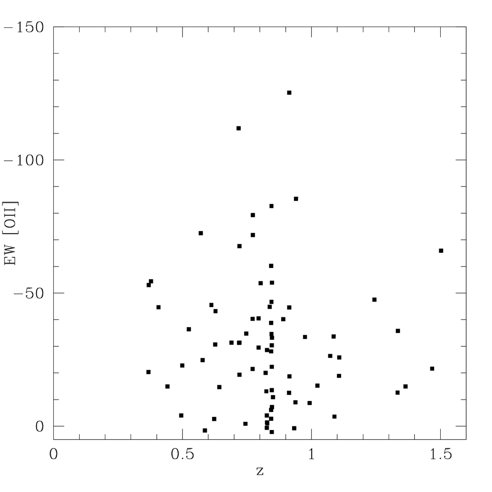
Figure 6: The rest equivalent widths of [OII] $\lambda$3727 versus redshift z for the field CL0023+0423.

The features which have equivalent widths measured are the $[{\rm OII}]\lambda 3727$ emission line, the absorption feature centered at 3835 Å (which includes CN, metal lines, Balmer H9), Balmer H8, the CaII H and K lines, H$\epsilon$, H$\delta$, the G-band, H$\gamma$, H$\beta$, and [OIII] $\lambda 5007$. These spectral features are prominent and, except for the last two, are located in a spectral range where the S/N is relatively good. To measure the equivalent width two “continuum” bands are defined on either side of the feature, and a continuum level is derived by linearly interpolating between the two bands. The equivalent width is then an integration of the continuum subtracted signal over a band centered on the feature. The continuum and line bands used for each feature are defined in Table 5. The observed spectra are shifted to zero redshift before carrying out the calculations. The equivalent widths are in Angstroms and are positive if the line is in absorption and negative if the line is in emission. The [OII] and [OIII] lines should be negative except for noise variations. Equivalent widths of the Balmer lines can be negative or positive. The rest-frame equivalent widths of $[{\rm OII}]\lambda 3727$, H$\beta$, and [OIII] $\lambda 5007$ are listed in columns 10, 11, and 12, respectively, of Tables 2 and 3. Errors in the equivalent widths of [OII], derived from the actual measurements in objects with no emission line, are about 4 Å ; any equivalent widths below this value are usually null detections. Errors for H$\beta$ and [OIII] are about 6 or 7 Å since they tend to lie redwards of 8000Å where the spectra are noisy, and the sky subtraction is difficult. The rest frame equivalent widths of [OII] are plotted against $z$ for the two cluster fields in Figures 6 and 7.

If we define active star formation by the presence of an [OII] line with an equivalent width of $\mathrel{\hbox{\raise 2.15277pt\hbox{$>$}\hbox to0.0pt{\hss\lower 2.15277pt\hbox{$\sim$}}}}15.0$ Å (as used by Hammer et al. 1997), 76% of the field (non-cluster) sample with redshifts of $z>0.$4 are active. Splitting this sample into the redshift bins of Hammer et al. (1997), we find that 79% of the field galaxies with $0.4\leq z<0.9$ are active, while 62% with $z\geq 0.9$ are active. In their field sample, Hammer et al. (1997) find 65% and 90% for the same redshift ranges. Since both samples are small, there is no significant difference. Of the CL0023+0423 and CL1604+4304 cluster members, 57% and 50% are active galaxies, respectively. These fractions are much larger, however, than the $\mathrel{\hbox{\raise 2.15277pt\hbox{$<$}\hbox to0.0pt{\hss\lower 2.15277pt\hbox{$\sim$}}}}15\%$ in clusters between $z=0.2$ and $z=0.55$ (Balogh et al. (1997)).

2.1.3 The 4000 Å Break and the Balmer Jump

The traditional estimator for the 4000 Å break amplitude is defined as the ratio of the integrated flux per unit wavelength in the rest band 4050–4250 Å to that in the rest band 3750–3950 Å (Bruzual 1983). One problem with this measurement is that it is substantially influenced by the overall color of the galaxy since the two measurements are separated by 300 Å. It also has some sensitivity to reddening. This traditional measurement works fairly well for early-type galaxies where (a) the spectrum is dominated by late-type stars, (b) the spectral energy distribution $f_{\lambda}$ is nearly constant so that the jump has only a small color term embedded in it, and (c) the jump is produced by metal line absorption between 3750 and 3980 Å.

For younger objects, such as those that we are dealing with in this paper, the Balmer jump can be much more important than the 4000 Å break. Hammer et al. (1997) introduced a Balmer jump index; however, it is simply a flux ratio in two bands and does not remove the overall color change. We, therefore, introduce a new definition of the break amplitude which is based on the flux between 3400 Å and 4280 Å. Two continuum bands, one from 3400–3700 Å and the other from 4050–4280 Å, are defined. The flux in each band is fitted by a first order equation. In practice, the two slopes that are generated are quite similar although they are not identical because of the intrinsic character of the spectrum and noise. The average of the two slopes is adopted for both bands and used to extrapolate the spectrum in each band to a rest wavelength of 3850 Å. The ratio of the two fits evaluated at 3850 Å defines the jump. Since we have extrapolated with the same slope, the measured jump is just the vertical separation between the two linear fits. (The wavelength for the fit is arbitrary since, by definition, the vertical separation is the same anywhere in the 3700–4000 Å range.) We will refer to this parameter as $J$ which is simply the intensity ratio expressed in magnitudes. The advantages of our $J$ estimator is that it can measure either the 4000 Å break or the Balmer jump. In addition, it is insensitive to redenning and to the slope of the energy distribution throughout the spectral range from 3400–4280 Å.

We use the analytic fit in the 3400–3700 Å region to extrapolate the flux between 3700 and 4000 Å. The ratio of the observed flux (in 50 Å segments) to this extrapolated flux is noted. If the jump is the Balmer jump, the ratios will increase rapidly between 3750 and 3875 Å and then stay relatively constant. If the jump is the 4000 Å break, the ratio stays close to unity from 3700 to 3950 Å and then quickly increases. The wavelength at which the intensity ratio increases from unity to the value corresponding to $J$ indicates whether it is the Balmer or 4000 Å jump or somewhere between the two. The measured jump ($J$) and the transition wavelength ($\lambda_{J}$), where measurable, are listed in column 13 of Tables 2 and 3. In addition, we have also calculated the traditional 4000 Å break D(4000) as defined above. These values are listed in column 14 of Tables 2 and 3.

2.2 Photometry

2.2.1 Broad Band Colors

The photometric survey was conducted in four broad band filters, $BVRI$, which match the Cousins system well. The response curves of these filters are shown in Figure 1 of Paper I. The Keck observations have been calibrated to the standard Cousins-Bessell-Landolt (Cape) system through exposures of a number of Landolt standard star fields (Landolt 1992). The FOCAS package (Valdes 1982) was used to detect, classify, and obtain aperture and isophotal magnitudes for all objects in the co-added $BVRI$ images. For each galaxy in the field, we have derived magnitudes in a circular aperture with a radius of $3^{{}^{\prime\prime}}$. This corresponds to a physical radius of $\{14.60~{}14.92\}~{}h^{-1}~{}{\rm kpc}$ at $z=\{0.84~{}0.90\}$, the redshifts of CL0023+0423 and CL1604+4304, respectively. The limiting magnitudes are $B=25.1$, $V=24.1$, $R=23.5$, and $I=21.7$ for a 5-$\sigma$ detection in our standard aperture (for more details, see Sects. 3.1 and 4.1 of Paper I). From these magnitudes, we have generated the corresponding AB values of ABB, ABV, ABR, and ABI using Equations 2–5 in Paper I. The corresponding AB values for all galaxies which have spectra are given in Tables 2 and 3 for the CL0023+0423 and CL1604+4304 fields, respectively.

2.2.2 Absolute Luminosities

One method for determining the absolute luminosities of distant galaxies is to use observed broad-band magnitudes and k-corrections. In our case this is very difficult as we are dealing with young objects at high redshifts where there are few observations from which to calculate the appropriate k-corrections. Instead, we make use of the fact that we have the observed AB magnitudes (see Sect. 2.2.1) and a best-fit evolutionary model to the energy distribution (for details on the evolutionary models and the fitting procedure, see Sect. 4) for each galaxy. We can relate apparent and absolute magnitude using the formalism of Equations 6, 9, and 10 in Gunn & Oke (1975). This relation becomes :

$$M_{AB_{\nu(1+z)}}=m_{AB_{\nu}}-2.5~{}{\rm log}~{}\left[\frac{9.00\times 10^{20}{\pounds}^{2}_{q}(z)(1+z)}{H_{o}^{2}}\right]$$ (1)

where ${\pounds_{q}(z)}$ is given in Equation 9 of Gunn & Oke (1975).

We can easily measure $m_{AB_{\nu}}$, the value of AB at the redshifted wavelength of the $B$ filter, for example. For a given $H_{o}$ and $q_{o}$, we can use this value to calculate the absolute magnitude at the rest $B$ wavelength from Equation 1 above. We have chosen to use a rest $B$ wavelength to eliminate or minimize any extrapolation. The absolute magnitude in this band is hereafter referred to as $M_{ABB}$. For redshifts of $z<0.92$ the redshifted $B$ filter position is within the observed wavelength range, and an interpolation of the best-fit evolutionary model can be made. Above $z=0.92$ the rest-frame $B$ filter wavelength is above the observed $I$ band, and an extrapolation is necessary. This extrapolation is done by using the best-fit evolutionary model to the four observed AB values (see Sect. 4) to extrapolate to the appropriate frequency. The uncertainty in the resulting absolute AB can be estimated from the uncertainty in the fit of the observations to the model.

We have done the calculations for $h=1.0$ where $h=H_{o}/100~{}{\rm km~{}s^{-1}~{}Mpc^{-1}}$ and for $q_{o}=0.1$ (e.g. Carlberg et al. 1996). The results are listed in Tables 2 and 3. For other values of $h$, simply add $5~{}{\rm log}~{}h$ to numbers in the tables.

3 Cluster Kinematics

One of the primary goals of the survey is an analysis of the kinematic properties of the clusters. We have acquired redshifts for $15-35$ cluster members in each system, enabling an accurate estimate of the cluster velocity dispersion to be made and, potentially, the cluster mass. Cluster velocity dispersions are calculated by first defining a broad redshift range, typically $\Delta z=\pm 0.06$, in which to conduct the calculations. This range is manually chosen to be centered on the approximate redshift of the cluster. We then compute the bi-weight mean and dispersion of the velocity distribution (Beers et al. (1990)) and identify the galaxy with the largest deviation from the mean. Velocity offsets from the mean are taken to be $\Delta v=c(z-\overline{z})/(1+\overline{z})$ which corrects for cosmological and relativistic effects. In the case of bi-weight statistics, $\overline{z}$ is the median of the distribution. If the galaxy with the largest velocity deviation differs from the bi-weight median by either more than 3$\sigma$ or by more than 3500 km s^-1, it is excluded and the computations are redone. The procedure continues until no further galaxies satisfy the above criteria. The 3500 km s^-1 limit is based on extensive data available for low $z$ clusters. For example, 95% of the galaxies within the central 3$h^{-1}$ Mpc region of the Coma cluster and with $cz\leq 12,000$ km s^-1 lie within $\pm 3500$ km s^-1 of the mean Coma redshift. This clipping procedure is conservative and does not impose a Gaussian distribution on the final redshift distribution: for CL0023+0423 we find that the resulting redshift distribution is inconsistent with a Gaussian at more than the 97% confidence level.

Figure 8 shows histograms of the velocity offsets relative to the mean cluster redshifts for the two clusters. In the case of CL1604+4304, the clipping procedure concludes after rejecting the 4 most deviant redshifts, all of which differ from the mean redshift (when the outlier is included in the computation) by more than 3500 km s^-1. We then get a mean redshift of $\overline{z}=0.8967$ and a dispersion of 1226 km s^-1 (corrected for cosmological effects) based on 22 galaxies. All dispersions quoted here have also been corrected for redshift measurement errors which are typically about 100 km s^-1 at $z\sim 0.9$, and the uncertainty in the dispersion is computed following the prescription of Danese et al. (1980). The Danese et al. prescription assumes the errors in velocity dispersions can be modeled as a $\chi^{2}$ distribution and that a galaxy’s velocity deviation from the mean cluster redshift is independent of the galaxy’s mass (i.e., the cluster is virialized). The angular and redshift distributions of the galaxies in CL1604+4304 show no obvious substructure (see Figure 4). In the case of CL0023+0423, the velocity dispersion is 1497 km s^-1 after the galaxies with velocity deviations of 3500 km s^-1 or greater are excluded (and the clipping process concludes because subsequent deviations are less than $3\sigma$). However, the galaxy distribution for CL0023+0423 shows clear bimodal structure in redshift space with peaks at $z=0.8274$ (7 galaxies) and $z=0.8453$ (17 galaxies), corresponding to a cosmologically-corrected velocity difference of $2922\pm 216$ km s^-1 (see Figure 8). These peaks are separated on the sky as well (see Figure 3). If we identify all CL0023+0423 galaxies with negative velocity offsets as belonging to separate group, we then find that the $z=0.8274$ system has a dispersion of 158 km s^-1 and the $z=0.8453$ system has a dispersion of 415 km s^-1. Table 6 gives the mean redshifts and dispersions for the clusters along with their errors.

The CL0023+0423 system highlights one of the inherent difficulties of studying cluster kinematics at high redshift – one requires at least 15 cluster members and, ideally, more before an accurate estimate of the velocity dispersion can be obtained. Figure 9 shows how the velocity dispersion for each cluster changes as the extreme outliers are sequentially excluded. The specific dispersion values discussed above are highlighted by arrow marks. The 95% confidence limits on our dispersions always overlap the adjacent value had we stopped the clipping process one step earlier or later.

3.1 Mass Estimation

A number of estimators are available for determining masses of virialized systems given a set of galaxy positions and redshifts. The pairwise mass estimator is defined as

$$M_{PW}={{3\pi}\over{G}}\sigma_{1}^{2}R_{h}$$ (2)

where $\sigma_{1}$ is the observed radial (1D) velocity dispersion and $R_{h}$ is the mean harmonic radius, defined as

$$R_{h}^{-1}=\left({{N(N-1)}\over 2}\right)^{-1}\sum_{i<j}{1\over{|r_{i}-r_{j}|}}$$ (3)

where $r_{i}$ and $r_{j}$ are the coordinates of the $i$th and $j$th galaxies and $N$ is the total number of galaxies. The mean harmonic radius tends to overweight close pairs but has the advantage that one does not need to specify a cluster center. Two estimators which tend to give somewhat more robust and accurate mass estimates are the projected mass estimator (Bahcall & Tremaine (1981); Heisler, Tremaine, & Bahcall (1985)) and the ringwise mass estimator (Carlberg et al. (1996)). The projected mass is defined as

$$M_{PM}={10.2\over{G(N-1.5)}}\sum_{i}(\Delta v_{i})^{2}R_{i}$$ (4)

where $\Delta v_{i}$ is the velocity offset of the $i$th galaxy from the mean cluster redshift and $R_{i}$ is its projected distance from the cluster center. The ringwise mass is defined as

$$M_{RW}={{3\pi}\over{2G}}\sigma_{1}^{2}R_{rw}$$ (5)

where $R_{rw}$ is

$$R_{rw}^{-1}=N^{-2}\sum_{i<j}c(k)/({\pi\over 2}[R_{i}+R_{j}])$$ (6)

where $R_{i}$ and $R_{j}$ are the projected distances from the cluster center of the $i$th and $j$th galaxies, $k=\sqrt{4R_{i}R_{j}/(R_{i}+R_{j})^{2}}$, and $c(k)$ is the complete elliptic integral of the first kind (Press et al. (1992)). The reader is referred to Carlberg et al. (1996) for further details.

For completeness, we compute mass estimates using all three methods and present the results in Table 6, along with the corresponding $1\sigma$ errors. In all cases, the pairwise mass estimate is the smallest value owing to the high weight given to close pairs (which tends to decrease the value of the harmonic radius and hence the mass). The projected and ringwise mass estimates are often in better agreement although the latter tends to produce the highest mass estimates.

For each system we generate mass estimates within the central 250$h^{-1}$ kpc and 500$h^{-1}$ kpc (so long as there is a sufficient number of galaxies within these bins) in addition to a mass estimate based on all the data shown in Figure 8. One obvious concern in evaluating the mass estimates in Table 6 is whether or not the clusters are indeed virialized. Recently, Small et al. (1998) have shown that most virial mass estimators do a reasonable job even when a bound system is not in equilibrium – estimates remain unbiased with a scatter of $\sim 25$% when $\delta\rho/\rho>5$. In the worst case, a virial mass estimate of a marginally bound (and, thus, unvirialized) system can be too high by not more than a factor of 2. The velocity histogram for CL1604+4304 is consistent with a Gaussian distribution (the probability that the observed redshift is drawn from a Gaussian distribution is 27.7%). For CL0023+0423, the velocity histograms are not well modeled by a Gaussian (probabilities $\mathrel{\hbox{\raise 2.15277pt\hbox{$<$}\hbox to0.0pt{\hss\lower 2.15277pt\hbox{$\sim$}}}}2.2$%).

The velocity dispersion and mass of CL1604+4304 are comparable with those in current epoch richness class 2 clusters. In the CL0023+0423 system, the high velocity component at $z=0.8453$ is significantly less massive and would be better compared with current epoch richness class 0 clusters, while the lower velocity component at $z=0.8274$ has a dispersion and mass which are comparable to local groups of galaxies (Zabludoff & Mulchaey 1998).

CL1604+4304 has also been detected in X-rays by the ROSAT PSPC (Castander et al. (1994)). Its X-ray luminosity is $L_{x}(0.1-2.4~{}{\rm keV})=2.70\pm 0.58\times 10^{43}~{}h^{-2}$ erg s^-1. Because of the large scatter in the local optical-X-ray relations, CL1604+4304 is consistent with the $L_{x}-\sigma$ relation of nearby clusters (Mushotsky & Scharf (1997)). However, its X-ray luminosity is low for its velocity dispersion and, therefore, the estimated cluster mass. A similar trend is observed in the Couch et al. (1991) optically-selected cluster sample at intermediate redshift. Bower et al. (1997) have examined several clusters from this sample in the range $0.38\leq z\leq 0.51$ and find that they also have higher velocity dispersions for a given X-ray luminosity. This may indicate that the galaxies and the gas are not in thermal equilibrium or that clusters at these earlier epochs are still experiencing significant infall.

3.2 Mass-to-Light Ratios

We use our BVR imaging to generate mass-to-light ratios. The luminosity in a given metric radius is

$$L=f(M_{Lim},\phi(M))\left[\left(\sum_{i}10^{0.4(m_{z}-m_{i}+A+K(z))}\right)-L_{bg}\right]$$ (7)

where the sum is over all galaxies within the prescribed radius, $m_{i}$ is the galaxy’s apparent magnitude, $A$ is a correction for galactic extinction, $K(z)$ is a k-correction, $m_{z}$ is a zeropoint adjustment to make the units absolute solar luminosities (and, thus, depends on the luminosity distance), $L_{bg}$ is a background subtraction, and $f(M_{Lim},\phi(M))$ is a correction for the unsampled faint end of the cluster luminosity function. We define $f(M_{Lim},\phi(M))$ to be

$$f(M_{Lim},\phi(M))=1+\left({{\int_{M_{Lim}}^{M_{Ref}}\phi(M)dM}\over{\int_{M_{Bright}}^{M_{Lim}}\phi(M)dM}}\right)$$ (8)

where we have assumed a Schechter form for $\phi(M)$ with $\alpha=-1.1$, $M_{Lim}$ is the absolute magnitude corresponding to the survey flux limit at the redshift of the cluster, $M_{Ref}=-10.2$, and $M_{Bright}=-26.5$. The background subtraction is based on deep galaxy counts performed by Gardner et al. (1996), Metcalfe et al. (1995) [for $B$-band]; Gardner et al. (1996), Smail et al. (1995) [for $V$ band]; and Smail et al. (1995) [for $R$-band]. Our own $BVR$ data on two non-cluster fields agrees well with the counts from these publications. We use the SED from the tau0.6 model (see §4.1) with a color age of 2 Gyr, the approximate mean color age of the cluster members (see Figures 12 and 13), to compute the appropriate k-corrections for each passband.

Tables 7 and 8 show the M/L ratios for the two cluster fields as functions of metric radius and passband. The uncertainties listed reflect the errors in the estimates of both the mass and the luminosity. For CL0023+0423, we compute results based on the centroid of the $z=0.8453$ component only. We use galaxies brighter than 25 mag in $B$, brighter than 24.5 mag in $V$, and brighter than 23.5 mag in $R$ for the cluster luminosity computations. As indicated above, however, all luminosities are corrected to reflect an integration to a common fiducial absolute luminosity given by $M_{Ref}$. The results in Tables 7 and 8 are based on $M^{*}_{B}=-19.4,\ M^{*}_{V}=-20.1,\ M^{*}_{R}=-21.0$, which are values appropriate for $z=0$ clusters. If we assume that $M^{*}$ evolves as $M^{*}(z)\approx M^{*}(0)-z$ (Lilly et al. (1995)), the M/L ratios increase by about 40%, 20%, and 14% in $B$, $V$, and $R$, respectively. The increase is a result of $f(M_{Lim},\phi(M))$ decreasing as $M^{*}$ decreases (becomes brighter).

The similarity of the M/L ratios in these two clusters to those in low $z$ clusters of similar richness suggests that cluster M/L ratios, at least in the central 500$h^{-1}$ kpc, have not changed much since $z\sim 0.8-0.9$. The uncertainties are large however and are dominated by uncertainties in the derived luminosity (e.g., the k-correction is a strong function of a galaxy’s age and morphology which makes it difficult to derive a precise luminosity without redshifts for many more cluster members than we currently have available here).

4 Comparison of Observations with Galaxy Evolutionary Models

In this section we compare the photometric and spectroscopic observations with synthetic models of galaxy evolution. The comparison of the models with the photometric observations yield what we refer to as “color ages”, while the comparison with the observed spectral properties yield “spectrum ages”. Both of these ages measure the time since the last period of major star formation. We have examined several different families of models. These families differ in their star formation scenarios and, therefore, give best-fit “ages” to the observations which are different. Consequently, the ages derived from this model fitting are not physical values but only parameters which characterize the data. To convert these model ages into real ages, we must choose, firstly, the family of models which fits best the observations and, secondly, the appropriate metal abundance. In this section, we have attempted to do this. Thirdly, we must estimate the amount of time between creation of the galaxy and the first period of star formation. This process is discussed in Sects. 5 & 6.

4.1 Galaxy Evolutionary Models

In order to establish the star formation history of the field and cluster galaxies, we compare the observed data to an appropriate set of spectrophotometric evolution models. We choose to use the Bruzual & Charlot (1995) family of stellar evolutionary models. These models are constructed using stars with solar metal abundances. This choice has the advantage that there exists a large database of spectra representing stars over the whole Hertzsprung-Russell diagram. The spectral energy distributions (SEDs) of the models fit very well the energy distributions measured for nearby present-age elliptical galaxies (Bruzual & Charlot (1993)), as well as galaxies in clusters with redshifts near 0.5 (Oke, Gunn & Hoessel 1996). In a practical sense the models are ideal since they include an absolute spectral energy distribution with a spectral resolution and range which is similar to that of our observations. The spectra can be converted directly to AB magnitudes, and broad-band AB values can be calculated (see Paper I). We have chosen models with a Salpeter luminosity function (Salpeter 1955) and a maximum stellar mass of $125~{}{\rm M_{\odot}}$. Comparisons with models constructed with a Scalo luminosity function (Scalo 1986) show no significant difference at the level of accuracy that we can achieve.

We also need to choose the model with the most appropriate star formation history. The simplest model is to assume that there is a large, initial burst of star formation after which the galaxy fades in accordance with passive stellar evolution models. These are called ssp models by Bruzual & Charlot. The next simplest models are those where star formation begins at $t=0.0$ and decreases exponentially with a fixed time constant. We have considered three such families of models with time constants of 0.3, 0.6, and 1.0 Gyr; these models are hereafter referred to as the tau0.3, tau0.6, and tau1.0 models, respectively.

In Figure 10 we have plotted the broad-band AB values, that is ABB, ABV, ABR, and ABI, as a function of log$\nu$ where $\nu$ is the frequency in Hz for a series of tau0.6 models of various ages ranging from 0 to 8 Gyr for a redshift of 0.897 (the redshift of the cluster in CL1604+4304). Over the age range from 0.05 to 6 Gyr, the models predict rapid and dramatic color evolution. However, there is very little color sensitivity with age beyond 6 Gyr as demonstrated by the similarity between the 6 and 8 Gyr curves. The broken curve in Figure 10 shows the energy distribution at 10 Gyr. It is virtually the same as the 8 Gyr curve. When the observed spectra have energy distributions in this range, we can only determine a minimum age. (The exact minimum age depends somewhat on the quality of the observations.) A similar family of curves can be plotted for the other models and for other redshifts. At a given redshift the predicted SEDs are very similar (provided that $z\geq 0.5$) except that the age at any color is somewhat different.

The Bruzual & Charlot models are also capable of generating detailed spectra. A sample of tau0.6 model spectra for different ages is shown in Figure 11. Here, the relative AB magnitudes are plotted against wavelength in Å. Within the age range shown in Figure 11, the most significant change with time, apart from the overall changes in color discussed above, is the variation in the strengths of the metal lines relative to the strengths of the Balmer lines.

4.2 Broad-Band Energy distributions

For each galaxy we have the four observed values ABB, ABV, ABR, and ABI. In addition, for any particular family of models (e.g. the tau0.6 models) we have the corresponding values of AB for each model age. We can now characterize the observations by finding the model with the age that best fits the observations. Since the relationship between AB and log $\nu$ for the models is not quite linear (see Figure 10), the fitting is done using a maximum likelihood technique. The broad-band energy distribution of each galaxy is then characterized by a single parameter which we will refer to as the color age. Since the uncertainty in the fitted color age is directly related to the uncertainty in the fitted linear slope, we use this relation to derive uncertainties in the color ages. The $1\sigma$ uncertainties are typically $0.1-0.4$ Gyr.

The above procedure has been carried out for several different families of models, including ssp, tau0.3, and tau0.6 models. As mentioned above, the resulting color ages are different for different models. Therefore, the color age should not be interpreted as a real age since some initial epoch. Rather it is a representative parameter which describes the energy distribution of a particular galaxy. Although the general progression of colors and spectral features with age are qualitatively similar for the ssp and various tau models, there are quantitative differences between them. Specifically, the relative strengths of spectral features are not coupled to the colors independently of the family of models. In an attempt to determine which model is more suited to our data, we have used the observational data for the confirmed cluster members. Firstly, we compare their observed spectral energy distributions (that is, the four AB values) with each model SED at the appropriate redshift in order to determine which model fits best. Using $\chi^{2}$ as a measure of the fit, we find that the tau0.3, tau0.6, and tau1.0 models provide equally good fits and are, in general, slightly better than the ssp models. The differences are small enough that we conclude that the color fits cannot be used to discriminate between models.

For reasons given in the next section, we have adopted the color ages provided by the tau0.6 family of models. The color age and the estimated error for each galaxy energy distribution, as derived using the tau0.6 model, are listed in columns 8 and 9 of Tables 2 and 3. Occasionally, the age is based on data from only three (or, in rare cases, two) passbands. As evident from Figure 10 and the derived ages listed in Tables 2 and 3, most of the fits occur in a domain where the models are changing rapidly with age. In a few cases the energy distributions imply ages which are sufficiently long that the energy distribution is insensitive to the model age. In these cases only a minimum model age can be derived (see Sect. 4.1).

4.3 Emission Line Strengths

In galaxies where star formation is ongoing or has occurred until very recently, the observed emission lines are primarily generated within HII regions. In a radiation limited case one has the classical Stromgren sphere. Every photon below the Lyman limit is absorbed by the ISM and eventually produces a Balmer line photon which can be observed in the visible spectrum. This argument was used by Zanstra (1931) to infer the flux beyond the Lyman limit of a star by measuring the Balmer line strength. This method has also been used by Kennicutt (1983) to calculate H$\alpha$ equivalent widths for studies of spiral galaxies. The excess energy of the original photon above the binding energy of HI is converted into kinetic energy in the surrounding gaseous nebula and, in equilibrium, reappears primarily in the forbidden lines of [OII], [OIII], etc. One complication which can arise is that absorption of visual and UV photons by dust and the subsequent re-radiation of this energy at IR wavelengths can upset the simple equilibrium of photons.

If dust absorption is negligible, one can readily calculate the equivalent width of a Balmer emission line and estimate the equivalent widths of the $[{\rm OII}]+[{\rm OIII}]$ emission lines, provided that the UV flux below the Lyman limit and the spectral energy distribution of the radiation in the visual is known. The Bruzual & Charlot models provide the necessary stellar flux information both below the Lyman limit and in the visible regime. In doing this calculation, we have represented the Lyman continuum flux by the flux at the Lyman limit multiplied by an appropriate bandwidth. This bandwidth was determined by integrating the model photon flux from the Lyman limit down to 250 Å and dividing by the flux at the Lyman limit. Our computations were done in detail only for the tau0.6 model with an age of 1 Gyr. This is adequate since the UV energy distributions relative to the flux at the Lyman limit are very similar for tau0.6 models of different ages. Assuming that 66% of the Balmer photons are H$\alpha$ and 17% are H$\beta$, the equivalent widths in Å for $\rm H\alpha$ and $\rm H\beta$ are found to be:

$$EW(\hbox{\rm H}\alpha) = 2483\frac{f_{\nu}(912)}{f_{\nu}(6563)}$$ (9)

$$EW(\hbox{\rm H}\beta) = 472\frac{f_{\nu}(912)}{f_{\nu}(4861)}$$ (10)

The calculation of the intensities and equivalent widths of the [OII] and [OIII] lines are much more complex. We have, therefore, used the models of McCall, Rybski & Shields (1985) to provide the ratios of intensities of these lines to that of H$\beta$. They interpret the variations in line strengths from one HII region to another to be due to oxygen abundance differences. In our case we are looking at a entire galaxy and presumably a large number of HII regions with different oxygen abundances. Consequently, we adopt a mean value for the oxygen abundance; their observations suggest that an abundance of 1.3 times the solar abundance is representative. Their calculated model for this case gives the desired line-intensity ratios (see Table 9). With the equivalent width of H$\beta$ as calculated from Equation 9 and the known energy distribution of the galaxy model, the equivalent widths of [OII] and [OIII]$\lambda 5007$ can readily be calculated. The results for a series of tau0.6 models of different ages are given in Table 9.

Searle (1971) and Baldwin et al. (1981) have also measured emission line ratios for many extragalactic HII regions. The model that we have chosen represents a mean of these data quite well. We have equivalent widths of [OIII]$\lambda 5007$ and H$\beta$ for some of our objects (see Tables 2 and 3). Although they usually have very large errors because they lie in the wavelength range 8000Å – 1$\mu$ where the spectra are noisy, they do cluster around the values selected in Table 9.

Since the strength of the [OII] emission line is an indicator of the star formation rate, its observed strength provides a guide as to whether an ssp or a tau model is a more appropriate model for making age estimates. If we fit an ssp model to the observed colors, we derive minimum possible ages. The strength of the rest $[{\rm OII}]$ equivalent width versus the ssp color age is shown in Figure 14 for the $z=0.8274$ and $z=0.8453$ objects in the CL0023+0423 field and the $z=0.8290$ and $z=0.8967$ objects in the CL1604+4304 field. The calculated emission-line equivalent widths indicate that for ssp models the ionizing flux decreases so rapidly with time that an emission line should not be visible after a model age of 0.02 Gyr. The fact that we do see emission lines in objects which have ssp model ages of at least one Gyr indicates that star formation must have continued for at least that long. This implies that strict ssp models are not valid for a majority of the galaxies; that is, these models do not produce enough star formation as a function of age.

Instead, consider a tau model which includes an exponentially decreasing star formation rate. Figure 15 is a plot similar to that in Figure 14, except that the color ages are derived from tau0.6 models. Table 9 lists the calculated equivalent width of the [OII] line for various galaxy ages in a tau0.6 model. These values are plotted as the solid line in Figure 15. This curve is essentially a negative exponential with a time constant of 0.6 Gyr since the strength of the [OII] line is controlled by the nearly instantaneous star formation rate. Within a factor of 2, the calculated curve represents very well the observed [OII] emission line strengths. The two points which are far to the right of the curve correspond to galaxies with poor spectra and uncertain redshifts. A similar plot with tau0.3 or tau1.0 models would show that the calculated curve fits the observations equally well. Therefore, we conclude that an exponentially decaying SFR is required to reproduce the amount of [OII] emission observed in our high-redshift sample. Such a star formation rate is most readily made with a tau model although models with a series of bursts which decrease in intensity or frequency with time would also work.

4.4 Analysis of the 4000Å Break and the Balmer Jump

We examine the relation between the break measure $J$ (defined in Sect. 2.1.3) and the color age as determined from the evolutionary models. Since the observed jumps are noisy for individual objects, a better comparison of the observational data with the models can be made by grouping galaxies together and averaging their spectra. The groups are selected using proximity in redshift and in color age, now crudely defined as young ($\leq$2 Gyr), medium (2-3 Gyr), and old ($\geq$3 Gyr). The jump ($J$) and the wavelength where the jump ($\lambda_{J}$) is centered of each average spectrum is calculated. The value of D(4000) is also determined. In Figure 16, we plot the resulting $J$ values (top panel), the wavelengths where the jump is centered $\lambda_{J}$ (middle panel), and the conventional 4000 Å break D(4000) [bottom panel] versus the logarithm of the color age as derived from fittings to the ssp models. Figure 17 shows a similar plot using the color ages derived from fitting to the tau0.6 models. We list the relevant values of this analysis for the tau0.6 models in Table 10. The group and the number of members used in each average spectrum are listed in columns 1 and 2. The mean color ages, the resulting jumps and the central wavelengths, and D(4000) are listed in columns 3, 6, and 7, respectively.

We can use the synthetic spectral energy distributions of the Bruzual & Charlot models described above to derive the theoretical relation between the break measure $J$ and the color age. The resulting relation for the ssp family of models is shown as the solid curve in the top panel of Figure 16. Between 0.1 and 0.3 Gyr the jump $J$ is the Balmer jump and corresponds to the dominant stars in the galaxy changing from B- to A-type stars. From 0.3 to 1.0 Gyr the dominant stars are later than A0, and the Balmer jump declines. From 1.0 to 4.0 Gyr the jump is the traditional 4000 Å break dominated by the CaII H and K lines and other strong metal lines. The wavelength where the jump occurs for the same ssp models is shown by the solid line in the middle panel of Figure 16. At left it is at 3875 Å and is due to the Balmer jump. At right it is at 4000 Å and is the traditional 4000 Å break. In the bottom panel, the solid curve represents the theoretical relation between D(4000) and color age for the ssp models. It should be noted that between 1.0 and 10.0 Gyr our value of $J$ is nearly constant, while the traditional 4000 Å jump D(4000) is still increasing (e.g., see Figure 13 of Bruzual & Charlot 1993). At lower ages D(4000) decreases rapidly as metal line absorption decreases, while $J$ actually increases because the Balmer Jump is large.

We have generated these relations for the tau0.6 family of models as well. The solid curves in Figure 17 show these relations. As expected, the results are similar, but the transitions occur at later color ages. The interpretation of the curves is analogous to that for the ssp models given above. A comparison of Figures 16 and 17 shows that the $J$ data fit the tau0.6 models better than the ssp models. However, for galaxies with smaller color ages, the measured jump is smaller than predicted by the models. This trend suggests that a tau model with a decay time constant even longer than 0.6 Gyr may be more appropriate. Indeed, the fit using a tau1.0 family of models does bring the observed points closer to the analytic curve. To summarize, the jump as measured by $J$ indicates that tau models are in general more appropriate than ssp models for galaxies with young color ages. For the oldest galaxies, either family of models is satisfactory.

The Bruzual & Charlot models assume solar metal abundances; however, we need to determine whether such models are appropriate for our data. We can do this by comparing the values of D(4000) predicted by various Bruzual & Charlot models to the observed values for the oldest galaxies in our sample. These galaxies are defined in lines 1, 4, 7 and 10 of Table 10. (We omit those galaxies in line 15 as their redshifts are $z<0.5$.) Averaging the data by the total number of galaxies in each line, we find that the observed–to–model ratio of D(4000) is $0.92\pm 0.05$ for the ssp models and $0.91\pm 0.06$ for the tau0.6 models. Here, we have assumed that the color ages which are listed as lower limits are actually 1 Gyr older; however, this changes the ratio by only 1–2%. The equivalent solar metal abundance models of Worthey (1994) give values of D(4000) which are about $7\%$ smaller than those of Bruzual & Charlot. Consequently, the observed–to–model ratios for the ssp and tau0.6 models of Worthey would be 0.98 and 0.97, respectively. We, therefore, conclude that our observations are consistent with solar abundances.

Worthey (1994) finds that D(4000) changes by about 12% when the abundance changes by 0.25 in the logarithm relative to solar. At the same time the overall colors of Worthey’s models also change by substantial amounts. Unfortunately, we are unable to make a detailed comparison to the models as the rest wavelength range defined by our colors is much shorter than that of Worthey; however, it is evident that the change in color with metal abundance approximately compensates for the change in D(4000). In other words, an ssp model with a metal abundance of -0.25 and an age of 1.5 Gyr gives the same color and D(4000) as a solar abundance model with an age of 3.0 Gyr. Since it is not possible to measure the metallicity directly with our data, we cannot separate age and metallicity. In other observations, Hammer et al. (1997) find a significant population of field galaxies at $z=0.7$ with small D(4000) indices which suggest lower than solar metal abundances or younger ages.

4.5 Ages Derived from Spectral Absorption Features

In addition to the color ages, a spectroscopic age estimate is obtained by comparing the equivalent widths of the seven selected spectral absorption features $\lambda$3835, H8, K, H, H$\delta$, G-band, and H$\gamma$ with those for the tau models. The best-fit spectroscopic-based age is then just that of the model with the minimum $\chi^{2}$ value. The resulting ages, however, are quite uncertain because the individual equivalent widths are themselves very uncertain. Therefore, we have decided not to estimate spectrum ages for individual galaxies, but rather to use the average spectra for the groups already defined in Table 10. For each averaged spectrum, an age is obtained from the maximum likelihood fit. In addition, we have also estimated a spectrum age by visually comparing the averaged data with the model spectra. The best fit was judged by eye, and the corresponding model age was noted. The visual estimate of the spectrum age and the best-fit spectrum age (along with the $\chi^{2}$ value) are listed in columns 4 and 5 of Table 10. A comparison of the color ages and spectrum ages shows reasonable agreement although the scatter is large. In these plots of color age versus spectrum age the scatter is lower for the visually determined spectrum ages than for the $\chi^{2}$ fitted ages, probably because the eye allows for inconsistencies in the apparent line strengths. As discussed in the previous section, we are unable to distinguish between spectrum age and metallicity for the reddest objects.

4.6 The Choice of Model

In Sect. 4, we have discussed the broad-band energy distributions, the emission line equivalent widths, the Balmer or 4000 Å jump $J$, the 4000 Å jump D(4000), and the absorption features in the galaxy spectra in terms of their consistency with the solar abundance Bruzual & Charlot families of models. Only the [OII] equivalent width and possibly the jump $J$ can serve to discriminate among the families of models. These spectral features, as observed, clearly rule out ssp models, but present good overall fits for the tau models. The color and spectrum ages also depend strongly on the assumed metallicity. Because there is no way to measure this with our data, we have chosen to calculate ages based on tau0.6 models with solar abundances (see Tables 2 and 3).

It should again be emphasized that the color and spectrum ages should not be interpreted as real ages since some initial epoch. The ages derived depend very much on the family of models and the assumed metallicity. That is, derived ages for tau1.0 models are older than those for tau0.6 models which are, in turn, older than the ssp models. The color age principally describes the overall color of the galaxy. To emphasize this, we note that the ages of galaxies within a single cluster show a large spread even though they are probably coeval (see Sect. 5). The cluster member ages could be made identical by using a different star-formation-rate decay time or a different metallicity for each individual galaxy. Since the calculated color is actually determined in the rest violet and ultraviolet regimes which is dominated by the more recently formed blue main sequence stars, the color age is really a measure of how long ago star formation was important. The [OII] equivalent width, on the other hand, represents the present star formation rate relative to this past star formation history.

5 Cluster Data

In this section, we examine the relationship between the estimated ages and other galaxy properties for the cluster and group members in the two fields. We use the ages derived from the colors, as they are considerably more precise than those derived from spectral features (see Sect. 4).

As noted in Table 6, the CL0023+0423 field contains two poor clusters or groups of galaxies at $z=0.8274$ and $z=0.8453$ with 7 and 17 known members, respectively. In CL1604+4304 there is a cluster with $z=0.8967$ with 22 known members. There is also a system of 8 galaxies with $z=0.8290$ which is most likely a sheet of galaxies given its distribution on the sky (see Figure 4). The rest [OII] equivalent widths are plotted against the tau0.6 model color ages for these galaxies in Figure 15. The figure shows that the [OII] equivalent widths are small for almost every galaxy with a color age greater than 2.5 Gyr. As expected, this implies that the reddest galaxies do not currently have significant star formation. We now plot in Figures 18 and 19 the tau0.6 color age versus the absolute magnitude $M_{ABB}$ (see Sect. 2.2.2) for the confirmed group/cluster members in CL0023+0423 and CL1604+4304, respectively. The reddest galaxies not only have very weak or absent [OII] emission, but they are the most luminous galaxies in the cluster. A similar result was found for field galaxies (Songaila et al. 1994). An obvious interpretation is that very luminous galaxies (and presumably very massive ones) begin star formation quickly and exhaust their gaseous component with an exponentially decreasing time constant of about 0.6 Gyr. Less massive galaxies convert gas to stars more slowly with an exponentially decreasing time constant which can be longer than 0.6 Gyr.

This correlation between age and luminosity is obvious in both groups of the CL0023+0423 system (Figure 18). In the high velocity component at $z=0.8453$, there are few luminous galaxies; correspondingly, there are only 2 (out of 17) galaxies which are red and old. In the low velocity component at $z=0.8274$, there are relatively more luminous galaxies and also relatively more (4 out of 7) cool, red objects. The location of these old, red galaxies in the cluster is also of some interest. In CL0023+0423 the two old galaxies of the $z=0.8453$ system are close together in the densest part of this group. The four red objects in the $z=0.8274$ system are also clumped together near the center of the group (see Figure 3). In the cluster of CL1604+4304 which contains the most old, red members, these galaxies are strung out in a line in the inner half diameter of the cluster (see Figure 4).

The only objects which can potentially yield model ages which are actual epochs are the reddest galaxies in the clusters. These galaxies have tau0.6 color ages of $\mathrel{\hbox{\raise 2.15277pt\hbox{$>$}\hbox to0.0pt{\hss\lower 2.15277pt\hbox{$\sim$}}}}3.8$ Gyr in Figures 18 and 19. These galaxies also make up the “red locus” observed in the color-magnitude diagrams of low and intermediate redshift clusters (e.g. Butcher & Oemler 1984; Aragón-Salamanca et al. 1991,1993; Stanford, Eisenhardt & Dickinson 1995,1997). HST observations indicate that these galaxies are typically early-type (elliptical or S0) galaxies. Similarly, we find that the red group/cluster members in our two fields are also classified as early spiral or early-type galaxies (see Paper III). These galaxies are fit well by either a single initial burst ssp model or by a tau model, such as tau0.6, where the star formation decay rate is rapid enough so that essentially no star formation has occurred within the last Gyr. Choosing those galaxies with accurate photometry and tau0.6 color ages of $>3.8$ Gyr, we find that there is one such object in the $z=0.8274$ group in the CL0023+0423 field, while there are five in the $z=0.8967$ cluster and one in the $z=0.8290$ structure in the CL1604+4304 field. These galaxies are listed in the footnote to Table 11 along with their galaxy classification where available (see Paper III).

The reddest of these galaxies have energy distributions for which the sensitivity to age is rapidly decreasing. All seven objects have been averaged to produce mean values of AB. Since all the galaxies have fairly similar measured apparent magnitudes, each galaxy has been given a weight of unity. The mean values of AB are listed in Table 11. The mean ABs have been fitted in the usual manner with solar metallicity ssp, tau0.6, and tau1.0 models. The ABs for the best fitting models are listed. The resulting ages and their estimated uncertainties (assuming solar metallicities) are also given in Table 11 along with the model values of AB. In all cases the fits are by no means perfect since the observations and the models have distinctly different curvatures. As expected the ssp ages are the shortest. The tau0.6 and tau1.0 model ages are longer and show that the derived age is very sensitive to the particular model. In a standard cosmology of $H_{o}=65$ and $q_{o}=0.1$, the age of the universe is 12.8 Gyr, and the age at $z=0.90$ is 5.8 Gyr. The ssp models, which we have already seen are not appropriate (see Sect. 4), give a time for the formation of the first stars at $2.5\pm 0.5$ Gyr after creation or $z\sim 3$. The tau0.6 models, which appear to fit the observed energy distributions and spectral features (see Sect. 4), give $0.8\pm 0.5$ Gyr ($z\sim 5$) which allows approximately 1 Gyr for the first stars to form. The tau1.0 models give ages which are much too long for this cosmology. If we had used a metallicity of $-0.25$, the ssp ages would have been about a factor of two smaller; the tau0.6 and tau1.0 ages would have been lower by less than a factor of two because tau models mix in young hot stars in which metallicity effects are smaller.

Most of the member galaxies with absent or weak [OII] emission have high color ages; however, there are a number of galaxies which appear to be young although they have very little [OII] emission. Their blue color and lack of [OII] emission indicate recent but no current star formation. Since star formation most likely occurs in bursts which exponentially decrease in intensity or frequency with time, these galaxies are just cluster members where the most recent burst occurred at least 0.1 Gyr ago.

6 Brightest Cluster Galaxies

The brightest cluster galaxy (BCG) in the CL0023+0423 system is in the low-velocity $z=0.8274$ group. It is Keck #2055 and has $M_{ABB}=-21.63+5~{}{\rm log}~{}h$. This galaxy is classified as an Sa(pec) and is shown in Figure 15 of Paper III. This group has an Abell richness class (RC) of 0 at best but is actually most similar in nature to a small group of galaxies (Zabludoff & Mulchaey 1998). The brightest cluster galaxy in the CL1604+4304 cluster at $z=0.8967$ is Keck #2855. It has $M_{ABB}=-21.91+5~{}{\rm log}~{}h$ and is classified as an Sa (see Figure 16 in Paper III). This cluster is quite rich, corresponding to an Abell richness class of about 2. Since not all of the galaxies in the fields were spectroscopically observed, we have checked to see if any other galaxy near the cluster (or group) centers which had not been observed could be the brightest cluster members. No candidates were found in either field. From (1) the color age of the galaxy, (2) the relation between color age and $B-V$ for the best-fit tau0.6 model, and (3) the conversion between ABB and $B$ given in Equation 3 of Paper I, we can derive the absolute rest luminosities of $M_{B}$ and $M_{V}$. These values for the two BCGs are listed in columns 4 and 5 of Table 12.

We compare the absolute luminosities of our BCGs to those in the nearby universe by examining the results of Schneider, Gunn & Hoessel (1983). For this comparison, we will compare the BCG in CL0023+0423 to a present-day ${\rm RC}=0$ BCG and the BCG in CL1604+42304 to a present-day ${\rm RC}=2$ BCG. Schneider, Gunn & Hoessel (1983) have measured and analyzed the brightest cluster galaxies in 84 Abell clusters. Using their definition of the reduced absolute magnitude (RAM) and converting their results to our default standard cosmology of $H_{0}=100$ and $q_{0}=0.1$, we find that the brightest cluster galaxy in a richness class 0 and 2 cluster at low redshift has a luminosity of $M_{g}=-21.13$ and $-21.41$, respectively (see column 7 of Table 12). We can convert the absolute luminosity $M_{g}$ to $M_{B}$ and $M_{V}$ using the conversion between the two passbands of $g$ and $B$, and the typical color of $B-V=0.97$ for the brightest cluster galaxies which are given in Schneider, Gunn & Hoessel (1983). The resulting values of $M_{B}$ and $M_{V}$ for a BCG in a low-redshift, richness class 0 and 2 cluster are given in columns 8 and 9, respectively, of Table 12. Based on the data presented in Table 12, we find that the brightening between $z=0.10$ (the mean redshift of the Schneider, Gunn & Hoessel sample) and $z\sim 0.90$ is $\Delta M_{B}=1.02$ and $\Delta M_{V}=0.85$. These results are identical for both the group in CL0023+0423 and the cluster in CL1604+4304; however, the accuracy of the magnitude differences is at best $0.2-0.3$ mag. This brightening is independent of the value of $H_{0}$ chosen. However, it does depend on $q_{0}$; that is, increasing $q_{0}$ from 0.1 to 0.5 would decrease the brightening by 0.37 mag.

We can use our best-fit tau0.6 models of these galaxies to calculate the expected brightening between $z=0.10$ and $z=0.90$. The results depend on both $q_{0}$ and $H_{0}$. We also assume that there is an interval of 1 Gyr between the time of creation and the time when star formation begins. For our standard values of $H_{0}=100~{}{\rm km~{}s^{-1}~{}Mpc^{-1}}$ and $q_{0}=0.1$, the brightening is 0.9 and 0.7 mag for $M_{B}$ and $M_{V}$, respectively. For $H_{0}=65$ and $q_{0}=0.1$ the predicted brightening is 0.8 and 0.7 mag, respectively. Given $H_{0}=65$, increasing $q_{0}$ to 0.5 increases the predicted brightening to 1.1 and 0.9 mag for $M_{B}$ and $M_{V}$, respectively. Since the standard deviations in the brightening of $M_{B}$ and $M_{V}$ are $\sim$0.2 mag, we find a formal value of $q_{0}=0.25\pm 0.25$ for $H_{0}=65$ provided the metallicity is solar. Similarly, Aragón-Salamanca et al. (1993) have looked for luminosity evolution in the brightest cluster galaxies using the infrared $K$ band. They have examined clusters at redshifts of $z\mathrel{\hbox{\raise 2.15277pt\hbox{$<$}\hbox to0.0pt{\hss\lower 2.15277pt\hbox{$\sim$}}}}0.90$, including CL1604+4304, but find no brightening. Our best-fit tau0.6 models predict that in $K$ the luminosity evolution should be about 60% of the luminosity evolution observed in $B$.

7 Galaxies at $z>0.9$

7.1 Luminosities

We have examined the highest redshift galaxies in our sample for those which may be of particular interest because of their spectral nature or luminosity. At these high redshifts, the luminosity brightening depends very strongly on $H_{0}$. Assuming a time of 1 Gyr for the first stars to form and $q_{0}=0.1$, the tau0.6 models predict a luminosity brightening in the brightest cluster galaxies of 1.6 mag for $H_{0}=100$ and 0.5 mag for $H_{0}=65$ between $z=0.90$ and $z=1.50$. For a reasonable Hubble constant $H_{0}=65$, almost all of the galaxies that we observed in this redshift range are no brighter than the predicted brightest cluster galaxies (see Sect. 6). However, there are a few interesting exceptions. At a redshift of $z=1.0908$ Keck #3152 in the CL0023+0423 field has an absolute luminosity of $M_{ABB}=-22.96$, nearly 1 mag brighter than a BCG at this redshift. This object, however, is a quasar or AGN. In addition, Keck #1023 ($z=1.2316$) in the CL1604+4304 field is about 0.2 mag brighter than expected; however, otherwise appears normal. Of special interest, Keck #3560 ($z=1.5029$) in the CL0023+0423 field and Keck #2858 ($z=1.3757$) in the CL1604+4304 field are 0.4 to 0.6 mag brighter than the expected luminosity of a BCG at these redshifts. These two objects also distinguish themselves by showing strong UV absorption lines. We discuss the implications of the ultraviolet lines of these two galaxies below.

7.2 Ultraviolet Absorption Lines

The MgII doublet at 2800 Å becomes visible in the models at an age of 0.5 Gyr and then strengthens rapidly (see Figure 11). Spectra taken with the Keck 10m telescope of the galaxy 53W091 at $z=1.55$ show this feature clearly (Dunlop et al. 1996). In addition, Cowie et al. (1995) observed these lines in a Keck spectrum of a $z=1.614$ galaxy. The MgII doublet is often seen in nearby star-forming and Seyfert 2 galaxies (Storchi-Bergmann, Kinney & Challis (1995); Kinney et al. (1996)). It is visible in all the spectra shown in Figure 5. In the older and redder objects this doublet is accompanied by numerous other absorption lines, the most prominent of which are 2881 Å due mainly to SiI and 2852 Å due mainly to MgI. Some of these lines can also be seen in the spectra of Figure 5. These features are strong in stars such as the sun and $\alpha$ Canis Minoris (Morton et al. 1977). At still shorter wavelengths, one finds the FeII resonance absorption lines at 2586.2 Å and 2600.2 Å. Keck spectra of a $z=1.614$ galaxy obtained by Cowie et al. (1995) and a $z=1.6036$ galaxy obtained by Koo et al. (1996) show these lines. These lines are often seen in nearby star-forming and Seyfert 2 galaxies with equivalent widths of $1-8$ Å for the combined $\lambda$2586, 2600 pair (Storchi-Bergmann, Kinney & Challis (1995); Kinney et al. (1996)). In our spectra they can be seen only when the redshift is well above 1.0, and the spectra have high signal-to-noise ratios. We detect these features in four objects in CL0023+0423 and three in CL1604+4304.

As shown in Figures 20 and 21, two galaxies, Keck #3560 in CL0023+0423 at $z=1.5029$ and Keck #2858 in CL1604+4304 at $z=1.3757$, not only have the two FeII resonance lines and the MgII 2800 Å feature, but they also have all the other resonance lines of FeII in multiplets UV1 to UV5 (Fuhr et al. 1988). Three of these lines were identified by Cowie et al. (1995) in the $z=1.614$ galaxy. All of these resonance lines are seen in HST spectra of high-redshift quasar including H821+643 and are caused by interstellar absorption in the Galaxy (Bahcall et al. 1992; Savage et al. 1993). Because in our case the lines are being created in distant galaxies, the question arises whether these lines originate in the atmospheres of the stars in the galaxy or whether they are of interstellar origin. The strongest argument for their interstellar origin is that only the true resonance lines are seen. Lines from slightly excited levels, such as $\lambda$2631 from multiplet UV1, are not seen. On the other hand, the strength of these features argues against an interstellar origin. The rest equivalent widths of the strongest interstellar FeII lines in the Galaxy are 1 to 2 Å (Bahcall et al. 1992; Savage et al. 1993). In Keck #3560 (CL0023+04323) the rest equivalent widths of $\lambda 2585$ and $\lambda 2601$ are 3.9 and 3.0 Å, respectively, while in the rather noisy spectrum of Keck #2858 (CL1604+4304) the combined pair has a total equivalent width of 13 Å. In our distant galaxies we are looking at a whole galaxy, and the range in velocity along the line-of-sight can be somewhat larger than in our own Galaxy. There appears, however, to be no way to generate sufficiently high velocities along the line-of-sight to produce interstellar lines with the large rest equivalent widths that we observe in Keck #3560 and #2858. In addition, these FeII lines are commonly seen in stars which should be present in these high-redshift galaxies. The strengths that we observe are comparable with the line strengths in star-forming and Seyfert 2 galaxies (Storchi-Bergmann, Kinney & Challis (1995); Kinney et al. (1996)). These lines are also strong in A-type stars such as Vega (Rogerson 1989) and Sirius (Rogerson 1987) and in early F-type stars such as $\alpha$ Aquilae (Morton et al. 1977). See also IUE spectra of B, A, and F type stars (Wu et al. 1991). We, therefore, conclude that the UV FeII and MgII lines must in fact be generated in the atmospheres of the young, hot stars in the galaxies.

8 Conclusions

In this paper, we have presented the results from a deep photometric and spectroscopic survey of two fields which are centered on the candidate, high-redshift clusters of CL0023+0423 at $z=0.84$ and CL1604+4304 at $z=0.90$. Based on these observations, we conclude the following :

• We have spectroscopically observed magnitude-limited (R $\leq 23.3$) samples of two fields with candidate clusters of galaxies at $z>0.8$. Both candidates are confirmed as real cluster-like density enhancements, but only $\sim 20$% of the observed galaxies are actually members of the clusters. The large foreground/background contamination is a common hazard when working in this redshift range and implies that one requires a minimum of $\sim 100-150$ redshifts per 15 square arcminutes if accurate kinematic parameters are desired.

• We find that the main cluster in the CL0023+0423 field consists of two components at nearly identical redshifts of $z=0.8274$ and $0.8453$ (corresponding to a radial velocity difference of $\sim 2900~{}{\rm km~{}s^{-1}}$). Their calculated velocity dispersions and corresponding masses indicate that these two components are more similar to groups or poor clusters of galaxies. In addition, the morphological analysis of Paper III indicates that these systems have a morphological composition which more closely resembles that of the field. The fraction of spiral galaxies is 66% or more. Though it is possible that these two groups are simply a chance projection on the sky, they may also be in the process of merging. The dynamics of the merging scenario is presented in another paper of this series (Lubin, Postman & Oke 1998).

• We have confirmed that there is a centrally-concentrated, rich cluster at $z=0.8967$ in the CL1604+4304 field. The velocity dispersion and implied mass are consistent with an Abell richness class 2 cluster. In addition, the morphological composition of CL1604+4304 is characteristic of a normal, present-day rich cluster. Early-type galaxies comprise 76% of the galaxies in the central $\sim$0.5 $h^{-1}~{}{\rm Mpc}$. In this population, the ratio of S0 to ellipticals is $\sim$1.7, consistent with galaxy populations found in local clusters (Paper III).

• The mass-to-light ratios in both clusters are similar to those seen locally but the uncertainties are high due to the sensitivity of the derived luminosity to the amount of color and luminosity evolution. Our k-corrected $R$-band M/L values are, none the less, significantly less (by $3-4\sigma$) than the zero redshift $R$-band M/L of $\sim 1300$ expected for an $\Omega=1$ universe.

• Defining active star formation as a rest equivalent width of [OII] $\lambda 3727$ which is greater than 15 Å, 79% of the field (non-cluster) galaxies with $0.4\leq z<0.9$ are active, while 62% with $z\geq 0.9$ are active. The fraction of field galaxies which have active star formation appears to be relatively independent of redshift. Of cluster members, 57% and 50% are active in the CL0023+0423 and CL1604+4304, respectively. These numbers are significantly higher than those of intermediate-redshift clusters (Balogh et al. 1997). Even though the cluster masses are very different in our two cases, the fractions of active galaxies are approximately the same; this suggests that star formation activity may not be a strong function of the cluster mass.

• The traditional estimator D(4000) of the 4000 Å break has been supplemented by a measurement $J$ which is color independent, measures either the Balmer jump or the 4000 Å break, and is able to distinguish between the two. For blue objects which have a Balmer jump, the measured jump is smaller than that predicted by standard Bruzual & Charlot models. For the old, red galaxies our measurements of D(4000) are consistent with the measured colors of the galaxies. Because changes in D(4000) are accompanied by compensating changes in color when the metallicity is varied, it is not possible to derive the metallicity from our data.

• We have compared our photometric and spectroscopic observations with various families of Bruzual & Charlot evolutionary models. The equivalent widths of the [OII]$\lambda 3727$ line show that models with a single burst of star formation followed by passive evolution (ssp models) are in most cases not satisfactory. However, models with an exponentially decreasing star formation rate after time zero (tau models) do predict the correct equivalent widths of [OII]; a time constant of 0.6 Gyr appears to be optimum. Our parameter $J$ also indicates that an exponentially decaying star formation model is better than the assumption of a single, monolithic burst.

• Fitting the observed spectra to the tau0.6 synthetic models indicate that the red galaxies, found mainly in the CL1604+4304 cluster at $z=0.8967$, have ages of $\sim 5$ Gyr for an assumed solar metallicity. For a cosmology of $H_{0}=65$ and $q_{0}=0.1$, this derived age allows nearly 1 Gyr between the time of creation and the first onset of star formation. Of the other Bruzual & Charlot models that we have examined, the tau1.0 models, which are otherwise acceptable, predict ages for these early-type galaxies which appear to be too old for this cosmology. The ages derived using ssp models, which we have shown are not generally appropriate for other observational reasons, give ages which are only $\sim 3$ Gyr. The morphological analysis presented in Paper III reveals that these old galaxies belong to the Hubble class of spheroid or early spiral galaxies. The derived ages are consistent with previous studies of high-redshift, early-type cluster members (Dickinson 1995; Stanford, Eisenhardt & Dickinson 1997).

• Comparing the brightest cluster galaxies in our clusters with those in Abell clusters of similar richness at redshifts of $z\sim 0.1$, we find a luminosity brightening of 1.02 mag for rest $M_{B}$ and 0.85 mag for rest $M_{V}$. For the same cosmological parameters above, the tau0.6 models predict a brightening of 0.8 and 0.7 mag for $M_{B}$ and $M_{V}$, respectively. Increasing $q_{0}$ from 0.1 to 0.5 increases the predicted brightening to 1.1 and 0.9 mag, respectively. At a given $q_{0}$, increasing $H_{0}$ also slightly increases the predicted brightening. Unlike the vast majority of their low-redshift counterparts, these two BCGs are disk systems (early-type spirals).

• Most of the field galaxies at $z>0.9$ have absolute luminosities which are not brighter than the predicted luminosity of a brightest cluster galaxy at the same redshift; however, there are two interesting exceptions. One galaxy at $z=1.5029$ in the CL0023+0423 field and one galaxy at $z=1.3757$ in the CL1604+4304 field are overluminous by nearly 1 mag compared with what is expected for brightest cluster galaxies at these redshifts. These galaxies have strong MgII$\lambda 2800$ absorption and FeII resonance line absorption. Although one argument suggests that in other galaxies these lines are mainly interstellar, they are too strong in these two galaxies for this to be the case. Therefore, they presumably come from late B-type stars in the galaxies.

Table 1: Information on Spectra

	CL0023+0423	CL1604+4304
(1) Number in sample	167	168
(2) Number not observed	39	31
(3) Number observed, no result	14	13
(4) Number of z=0.000 cases	6	20
(5) QSOs	2	1
(6) Number with significant redshifts	106	103
(7) Number with emission lines	94	81

Table 2: Objects with Spectra in the CL0023+0423 Field

n	ABB	ABV	ABR	ABI	z	Qual	colage	err	EW[OII]	EW($H\beta$)	EW[OIII]	Jump($\lambda_{J}$)	D(4000)	$M_{ABB}$
30	23.91	23.33	22.64	21.44	0.8470	4	1.8	0.2	-7.2	2.5	15.3	0.36(3900)	1.10	-20.41
40	23.82	23.09	22.66	22.16	0.3307	4	1.0	0.3	$\cdots$	-0.6	-10.8	$\cdots$	$\cdots$	-17.14
53	$\cdots$	$\cdots$	22.74	22.12	0.8435	4	0.4	0.2	-6.1	-20.3	16.7	0.99(3875)	1.46	-19.91
96	24.74	23.64	22.88	21.37	0.6230	4	3.4	0.4	-2.7	0.2	4.5	$\cdots$	1.58	-19.15
134	24.06	23.96	23.81	21.95	0.8027	4	1.1	0.2	-53.7	$\cdots$	$\cdots$	0.39(0—0)	$\cdots$	-19.35
145	24.04	23.70	23.77	22.18	1.0730	2	1.4	0.3	-26.4	$\cdots$	$\cdots$	-0.16(0—0)	1.31	-20.70
157	26.16	24.71	26.43	22.32	0.8447	1	3.6	2.0	-46.7	-5.2	12.9	0.80(3850)	1.21	-19.52
194	24.10	24.05	23.49	22.53	9.0000	$\cdots$	$\cdots$	$\cdots$	$\cdots$	$\cdots$	$\cdots$	$\cdots$	$\cdots$	$\cdots$
217	24.58	23.73	23.02	21.85	0.8514	1	2.2	0.3	-10.9	-8.2	17.4	-0.28(0—0)	1.44	-20.06
264	23.15	22.52	21.93	21.36	0.7946	4	1.4	0.1	-40.5	38.1	33.9	0.22(0—0)	1.14	-20.62
394	23.73	23.45	22.78	22.94	0.7947	4	1.1	0.2	-29.5	30.9	22.0	$\cdots$	$\cdots$	-19.71
451	24.18	23.43	22.81	21.95	9.0000	$\cdots$	$\cdots$	$\cdots$	$\cdots$	$\cdots$	$\cdots$	$\cdots$	$\cdots$	$\cdots$
468	23.90	23.25	22.70	21.68	0.7718	4	1.7	0.2	-21.5	-42.9	-18.6	$\cdots$	1.66	-19.90
509	$\cdots$	$\cdots$	22.47	21.57	0.8458	4	0.8	0.3	-13.5	2.7	5.4	0.18(0—0)	1.09	-20.30
557	24.18	23.49	23.47	23.46	0.3642	4	0.4	0.3	$\cdots$	-6.9	-26.4	$\cdots$	1.38	-16.78
569	24.25	24.13	23.46	22.22	0.7180	1	1.1	0.2	-111.9	-79.9	38.7	$\cdots$	$\cdots$	-18.79
588	25.17	24.41	23.26	21.40	9.0000	$\cdots$	$\cdots$	$\cdots$	$\cdots$	$\cdots$	$\cdots$	$\cdots$	$\cdots$	$\cdots$
605	24.70	24.28	23.96	22.32	9.0000	$\cdots$	$\cdots$	$\cdots$	$\cdots$	$\cdots$	$\cdots$	$\cdots$	$\cdots$	$\cdots$
644	23.79	23.07	22.86	22.31	0.0260	1	3.5	1.6	$\cdots$	$\cdots$	$\cdots$	$\cdots$	$\cdots$	-10.76
658	24.11	23.54	22.85	22.11	0.9150	2	1.8	0.3	-18.7	7.3	10.8	0.74(3950)	1.18	-20.45
701	20.68	19.91	19.57	19.03	0.2388	4	2.0	0.2	$\cdots$	-7.0	-4.9	$\cdots$	$\cdots$	-19.42
702	24.01	23.53	23.02	22.09	0.6266	4	1.0	0.2	-30.7	5.9	-18.2	0.83(3800)	$\cdots$	-18.61
792	24.82	24.35	23.38	21.72	0.6432	4	2.6	0.4	-14.7	-9.7	-7.3	0.53(3950)	1.41	-18.81
805	23.97	23.82	23.29	$\cdots$	1.0886	3	1.6	0.3	-3.6	$\cdots$	$\cdots$	0.49(0—0)	1.14	-20.83
825	22.84	22.35	22.11	21.83	0.4436	4	0.3	0.1	22.2	-16.8	-81.4	$\cdots$	$\cdots$	-18.47
926	23.65	23.23	22.72	21.90	0.6900	4	1.0	0.2	-31.4	-8.0	3.8	0.63(3775)	1.39	-19.24
946	25.86	25.31	25.12	22.99	0.7213	2	2.0	1.0	-19.3	-22.9	-4.6	$\cdots$	1.61	-17.91
980	22.53	23.74	23.46	22.08	1.4870	1	0.3	$\cdots$	$\cdots$	$\cdots$	$\cdots$	$\cdots$	$\cdots$	-21.25
984	24.52	22.85	$\cdots$	$\cdots$	0.0000	$\cdots$	$\cdots$	$\cdots$	$\cdots$	$\cdots$	$\cdots$	$\cdots$	$\cdots$	$\cdots$
1052	24.38	22.53	20.16	19.82	0.7445	4	$\geq$5.0	$\cdots$	-0.9	2.0	25.8	0.54(4000)	1.79	-21.84
1099	23.46	22.81	22.63	22.01	0.2700	4	0.6	0.3	$\cdots$	-13.0	-51.1	$\cdots$	$\cdots$	-16.77
1104	22.82	22.47	21.82	20.75	0.4010	4	1.8	0.2	$\cdots$	-22.1	-86.6	$\cdots$	$\cdots$	-18.68
1124	$\cdots$	21.65	21.14	19.88	0.4005	4	$\geq$6.0	$\cdots$	$\cdots$	-10.9	-89.0	$\cdots$	$\cdots$	-19.33
1230	25.70	24.39	23.50	21.42	0.9330	4	$\geq$4.0	$\cdots$	0.8	6.7	-8.2	0.51(4000)	1.74	-20.61
1253	23.99	23.53	22.94	21.75	0.8458	4	1.6	0.2	-22.3	-5.0	3.6	0.64(3850)	0.86	-20.03
1266	23.30	22.83	22.51	20.78	9.0000	$\cdots$	$\cdots$	$\cdots$	$\cdots$	$\cdots$	$\cdots$	$\cdots$	$\cdots$	$\cdots$
1302	24.02	23.19	23.39	22.17	9.0000	$\cdots$	$\cdots$	$\cdots$	$\cdots$	$\cdots$	$\cdots$	$\cdots$	$\cdots$	$\cdots$
1330	21.99	21.80	21.74	21.22	0.2541	1	0.1	0.1	$\cdots$	0.8	-0.4	$\cdots$	$\cdots$	-17.64
1336	22.93	22.35	21.83	21.23	0.5776	4	1.0	0.1	-24.8	-0.7	2.9	0.47(4000)	1.19	-19.50
1374	24.28	23.91	24.38	22.51	0.8442	1	0.9	0.3	-60.2	-14.2	15.5	0.58(3850)	1.24	-19.16
1375	23.06	22.68	22.36	21.65	0.6284	4	0.6	0.1	-43.2	-17.3	-37.8	0.80(3875)	1.09	-19.22
1392	23.49	23.09	22.84	22.15	0.9142	1	1.0	0.1	-125.3	-1.8	11.5	$\cdots$	$\cdots$	-20.33
1412	23.40	22.95	$\cdots$	$\cdots$	0.9137	2	1.6	0.2	-44.6	2.6	$\cdots$ .9	0.98(3875)	1.25	-20.94
1453	23.37	22.89	22.45	21.82	0.7725	3	1.1	0.1	-40.3	-39.7	-8.9	0.48(3800)	1.14	-20.01
1470	24.61	23.99	23.52	22.17	0.4416	4	2.0	0.5	-14.9	1.9	-29.3	0.36(0—0)	$\cdots$	-17.37
1478	24.02	23.77	24.09	22.46	0.7732	1	0.6	0.1	-79.3	11.1	-0.8	$\cdots$	$\cdots$	-18.76
1511	23.90	23.88	23.50	22.48	1.3351	2	1.8	0.3	-35.8	$\cdots$	$\cdots$	$\cdots$	$\cdots$	-21.62
1526	22.66	21.97	21.51	21.07	0.4083	4	1.0	0.1	$\cdots$	-6.3	-14.3	$\cdots$	$\cdots$	-18.87
1534	23.75	23.34	23.08	22.05	9.0000	$\cdots$	$\cdots$	$\cdots$	$\cdots$	$\cdots$	$\cdots$	$\cdots$	$\cdots$	$\cdots$
1552	21.62	20.94	20.67	20.37	0.1852	4	1.4	0.1	$\cdots$	-1.7	-8.7	$\cdots$	$\cdots$	-17.63
1566	24.18	23.75	23.55	22.17	0.8470	4	1.1	0.3	-53.9	-7.0	-29.2	0.85(3800)	1.51	-19.49
1572	20.73	20.06	19.81	19.46	0.1851	4	1.4	0.1	$\cdots$	-1.6	-4.5	$\cdots$	$\cdots$	-18.53
1628	23.31	22.55	22.35	21.84	0.5875	1	0.9	0.1	1.6	-27.7	8.9	-0.19(0—0)	$\cdots$	-19.15
1659	23.65	23.17	22.96	22.25	0.5708	4	0.6	0.2	-72.5	-19.0	-83.7	$\cdots$	1.18	-18.41
1662	23.28	22.73	22.16	21.01	9.0000	$\cdots$	$\cdots$	$\cdots$	$\cdots$	$\cdots$	$\cdots$	$\cdots$	$\cdots$	$\cdots$
1689	23.47	23.36	23.21	22.04	1.4679	2	2.0	0.2	-21.6	$\cdots$	$\cdots$	$\cdots$	$\cdots$	-22.49
1699	24.60	23.26	22.37	20.91	0.8435	4	3.5	0.2	-2.8	5.4	-2.7	0.33(3975)	1.53	-20.93
1749	23.51	22.95	22.92	22.25	0.0811	1	1.6	0.4	$\cdots$	1.8	-0.5	$\cdots$	$\cdots$	-13.62
1832	24.05	23.68	$\cdots$	$\cdots$	9.0000	$\cdots$	$\cdots$	$\cdots$	$\cdots$	$\cdots$	$\cdots$	$\cdots$	$\cdots$	$\cdots$
1833	23.81	23.04	22.39	20.91	9.0000	$\cdots$	$\cdots$	$\cdots$	$\cdots$	$\cdots$	$\cdots$	$\cdots$	$\cdots$	$\cdots$
1846	24.34	24.53	23.19	21.08	0.8465	2	2.7	0.2	2.2	1.1	20.4	0.46(3950)	1.34	-20.50
1912	24.56	24.22	23.12	21.76	0.8444	3	2.2	0.4	-38.8	-19.4	25.2	0.46(3975)	1.14	-19.95
1921	24.31	23.71	23.01	21.93	0.8456	4	1.8	0.3	-30.4	3.8	4.8	0.83(3825)	1.03	-19.92
1922	23.07	22.90	22.94	21.95	1.3341	2	1.3	0.2	-12.6	$\cdots$	$\cdots$	$\cdots$	$\cdots$	-21.93
1949	24.54	23.74	$\cdots$	$\cdots$	9.0000	$\cdots$	$\cdots$	$\cdots$	$\cdots$	$\cdots$	$\cdots$	$\cdots$	$\cdots$	$\cdots$
1968	23.59	23.54	23.11	22.48	9.0000	$\cdots$	$\cdots$	$\cdots$	$\cdots$	$\cdots$	$\cdots$	$\cdots$	$\cdots$	$\cdots$
1971	22.96	22.61	22.19	21.45	1.1074	4	1.6	0.1	-18.9	$\cdots$	$\cdots$	0.99(3850)	1.28	-22.07
2003	22.93	22.40	22.47	21.71	0.2480	4	0.3	0.2	$\cdots$	-3.5	-22.2	$\cdots$	$\cdots$	-16.88
2035	24.22	23.88	22.44	20.60	0.8274	4	3.5	0.2	0.6	3.3	-4.1	0.69(4000)	1.84	-20.95
2055	24.11	22.66	21.71	20.06	0.8266	4	3.9	0.2	-4.0	6.7	3.1	0.64(3975)	1.56	-21.63
2075	23.25	22.97	22.96	21.72	0.8447	4	0.8	0.1	-82.7	-12.4	-98.6	0.08(0—0)	0.94	-20.02
2092	24.25	23.78	22.78	22.11	0.5162	3	1.5	0.4	$\cdots$	-27.3	-0.1	$\cdots$	1.04	-18.12
2103	24.09	23.53	23.23	22.05	0.3524	4	1.1	0.3	$\cdots$	-23.4	-87.5	$\cdots$	$\cdots$	-17.05
2108	23.56	23.19	23.71	21.97	0.9375	2	0.8	0.1	-9.0	-10.6	-2.9	$\cdots$	$\cdots$	-20.19
2110	23.43	23.07	23.06	21.91	1.0858	4	1.1	0.1	-33.7	$\cdots$	$\cdots$	0.54(3950)	1.29	-21.00
2121	23.56	22.85	22.24	21.09	0.8281	4	1.9	0.2	-1.4	35.6	2.6	0.84(3900)	1.05	-20.67
2144	23.69	23.32	22.84	22.45	0.8444	2	1.1	0.2	-28.1	$\cdots$	23.1	0.59(3875)	1.26	-20.01
2166	23.93	22.94	22.20	20.94	0.8288	3	2.6	0.2	-1.1	2.4	-4.8	0.43(4000)	1.38	-20.85
2182	22.01	21.37	$\cdots$	$\cdots$	0.0000	4	$\cdots$	$\cdots$	$\cdots$	$\cdots$	$\cdots$	$\cdots$	$\cdots$	$\cdots$
2212	23.37	22.66	22.09	21.29	0.3297	4	1.9	0.2	$\cdots$	-5.3	-22.9	$\cdots$	$\cdots$	-17.71
2213	24.04	23.76	23.27	22.64	0.8380	2	1.0	0.2	-44.8	4.4	1.6	0.48(3825)	1.09	-19.52
2232	$\cdots$	23.02	22.29	21.29	0.9931	1	1.8	0.1	-8.7	$\cdots$	$\cdots$	0.27(3850)	1.10	-21.41
2271	23.86	23.12	$\cdots$	$\cdots$	0.3528	4	0.6	$\cdots$	$\cdots$	-3.9	-42.2	$\cdots$	$\cdots$	-17.13
2336	24.96	$\cdots$	25.23	22.46	0.8251	1	1.7	0.5	-13.1	-7.1	-33.3	$\cdots$	$\cdots$	-19.29
2348	22.49	21.63	21.24	20.86	0.8474	4	1.3	0.1	-33.2	-18.8	22.0	0.45(3775)	1.38	-21.49
2400	23.66	23.36	23.23	22.02	1.1079	2	1.3	0.2	-25.8	$\cdots$	$\cdots$	0.16(0—0)	0.90	-20.92
2415	24.79	23.75	23.43	21.68	0.8451	4	2.4	0.3	-34.6	2.6	16.4	-0.20(0—0)	1.29	-19.97
2433	22.83	22.27	22.05	21.77	0.2388	4	0.6	0.2	$\cdots$	-6.7	-28.7	$\cdots$	$\cdots$	-17.01
2477	24.06	23.31	23.09	22.10	0.1034	2	2.8	1.0	$\cdots$	1.6	23.1	$\cdots$	$\cdots$	-13.77
2548	23.99	23.27	23.01	22.14	0.2208	3	1.6	0.4	$\cdots$	3.5	2.8	$\cdots$	$\cdots$	-15.79
2563	23.01	22.29	22.40	21.41	9.0000	$\cdots$	$\cdots$	$\cdots$	$\cdots$	$\cdots$	$\cdots$	$\cdots$	$\cdots$	$\cdots$
2598	23.52	23.13	22.22	22.20	9.0000	$\cdots$	$\cdots$	$\cdots$	$\cdots$	$\cdots$	$\cdots$	$\cdots$	$\cdots$	$\cdots$
2615	23.63	23.30	22.61	22.17	0.6124	4	0.9	0.2	-45.5	-3.3	-9.5	$\cdots$	1.92	-18.83
2616	24.00	23.54	22.99	22.03	0.7193	4	1.2	0.2	-31.3	-29.5	1.3	0.89(3875)	0.88	-19.14
2640	24.63	24.07	23.53	22.19	0.9131	4	1.9	0.3	-12.5	-6.8	-19.0	0.94(4000)	1.34	-19.95
2664	23.69	23.43	22.84	22.07	0.7208	4	0.9	0.1	-67.6	-108.2	-102.7	$\cdots$	$\cdots$	-19.20
2680	23.84	23.29	22.83	21.60	1.0235	3	1.9	0.2	-15.2	$\cdots$	$\cdots$	0.33(3850)	1.51	-21.12
2733	24.02	23.62	23.34	22.39	0.4072	4	0.5	0.2	-44.7	-21.9	-66.3	$\cdots$	1.13	-17.15
2764	24.06	23.46	23.14	22.41	0.7210	1	1.1	0.2	-31.4	6.9	-19.4	$\cdots$	1.17	-19.10
2773	23.35	22.92	22.93	22.14	0.9404	2	0.7	0.1	-85.4	15.3	-1.9	0.23(0—0)	0.98	-20.39
2792	23.20	22.32	22.03	21.76	0.2983	4	1.0	0.3	$\cdots$	4.4	-7.9	$\cdots$	$\cdots$	-17.54
2798	24.59	23.81	23.46	22.05	0.9752	1	2.0	0.7	-33.5	$\cdots$	$\cdots$	0.38(4000)	$\cdots$	-20.49
2832	23.81	23.54	23.02	22.15	1.3645	4	1.4	0.2	-14.9	$\cdots$	$\cdots$	$\cdots$	$\cdots$	-21.01
2872	23.82	23.66	23.60	22.50	2.5950	4	$\cdots$	$\cdots$	$\cdots$	$\cdots$	$\cdots$	$\cdots$	$\cdots$	$\cdots$
2924	25.93	24.46	23.30	21.17	0.0000	$\cdots$	$\cdots$	$\cdots$	$\cdots$	$\cdots$	$\cdots$	$\cdots$	$\cdots$	$\cdots$
2986	23.45	23.21	23.07	22.12	1.2436	4	1.5	0.2	-47.5	$\cdots$	$\cdots$	$\cdots$	$\cdots$	-21.59
3045	23.85	23.04	22.82	22.28	0.2971	1	0.8	0.4	$\cdots$	-10.5	1.1	$\cdots$	$\cdots$	-16.80
3075	24.35	23.42	22.86	22.24	0.3306	4	2.4	0.7	$\cdots$	-5.3	-13.2	$\cdots$	$\cdots$	-16.87
3079	24.64	23.65	23.20	22.01	0.0000	4	$\cdots$	$\cdots$	$\cdots$	$\cdots$	$\cdots$	$\cdots$	$\cdots$	$\cdots$
3083	23.92	22.97	22.56	22.21	0.3356	4	1.4	0.5	$\cdots$	2.7	-10.6	$\cdots$	$\cdots$	-17.27
3108	24.21	23.36	23.24	22.13	0.3683	4	1.2	0.5	-20.3	-9.7	-39.3	$\cdots$	1.43	-17.14
3119	23.91	23.72	23.20	22.77	0.4989	1	0.3	0.2	-22.8	-12.1	10.2	0.85(3875)	0.88	-17.54
3128	23.69	23.03	$\cdots$	$\cdots$	0.3779	4	0.6	$\cdots$	-54.4	-64.3	-277.2	$\cdots$	$\cdots$	-17.46
3152	23.16	22.56	$\cdots$	$\cdots$	1.0908	1	3.0	$\cdots$	$\cdots$	$\cdots$	$\cdots$	$\cdots$	$\cdots$	-22.96
3175	$\cdots$	22.78	22.38	21.55	0.8280	4	0.9	0.2	-28.6	0.3	-17.4	0.86(3825)	1.03	-20.30
3265	21.71	20.35	19.62	18.17	0.0000	$\cdots$	$\cdots$	$\cdots$	$\cdots$	$\cdots$	$\cdots$	$\cdots$	$\cdots$	$\cdots$
3371	24.30	24.08	24.30	22.13	0.7472	4	1.2	0.3	-34.8	-1.5	-6.0	0.33(3825)	1.25	-18.93
3416	24.10	23.78	23.19	22.17	0.7734	2	1.1	0.2	-71.8	9.1	-59.2	0.68(3850)	1.12	-19.23
3435	23.11	22.77	$\cdots$	$\cdots$	0.4953	4	0.5	$\cdots$	-4.0	-0.9	2.7	$\cdots$	$\cdots$	-18.50
3436	23.91	23.66	23.49	22.49	0.8906	2	0.8	0.2	-40.2	19.0	-4.3	0.05(0—0)	0.98	-19.59
3465	25.31	23.93	$\cdots$	$\cdots$	0.0000	4	$\cdots$	$\cdots$	$\cdots$	$\cdots$	$\cdots$	$\cdots$	$\cdots$	$\cdots$
3508	22.14	21.44	21.15	21.10	0.1471	4	1.4	0.2	$\cdots$	1.3	-7.3	$\cdots$	$\cdots$	-16.56
3560	23.19	22.96	22.79	22.12	1.5029	3	2.0	0.2	-65.9	$\cdots$	$\cdots$	$\cdots$	$\cdots$	-22.88
3611	23.36	22.91	22.54	21.40	0.8224	2	1.3	0.1	-20.0	$\cdots$	-1.6	0.46(4000)	1.37	-20.37
3640	24.35	24.04	23.35	22.33	0.3690	4	1.1	0.4	-53.0	-0.2	-4.8	$\cdots$	$\cdots$	-16.87
3671	24.15	23.76	23.36	22.39	0.5248	4	0.7	0.2	-36.4	-7.7	-33.5	$\cdots$	0.99	-17.78
3703	22.41	21.49	20.92	20.53	0.3604	4	1.9	0.2	$\cdots$	-5.5	-9.5	$\cdots$	$\cdots$	-19.05

Table 3: Objects with Spectra in the CL1604+4304 Field

n	ABB	ABV	ABR	ABI	z	Qual	colage	err	EW[OII]	EW($H\beta$)	EW[OIII]	Jump($\lambda_{J}$)	D(4000)	$M_{ABB}$
98	$\cdots$	$\cdots$	26.82	22.44	0.3459	1	$\cdots$	$\cdots$	$\cdots$	-4.9	-0.7	$\cdots$	$\cdots$	$\cdots$
142	23.56	23.24	22.48	21.15	0.8216	2	1.6	0.1	-39.0	6.1	1.4	$\cdots$	0.93	-20.39
144	22.64	22.26	21.75	20.93	0.6825	1	1.0	0.1	-20.4	-0.9	-14.6	0.63(3850)	1.18	-20.18
205	24.01	24.02	22.74	21.60	0.4258	4	2.2	0.2	$\cdots$	-4.0	-26.4	$\cdots$	$\cdots$	-17.87
293	23.48	23.44	22.85	21.49	0.9748	1	1.4	0.2	-57.9	11.6	$\cdots$	$\cdots$	$\cdots$	-20.98
320	23.44	23.22	22.71	21.40	0.9738	2	1.4	0.2	-77.1	12.8	$\cdots$	$\cdots$	$\cdots$	-21.05
336	23.64	22.62	21.96	20.80	0.3018	4	5.0	1.0	$\cdots$	-6.5	-4.0	$\cdots$	$\cdots$	-17.51
343	24.11	23.81	22.41	21.16	0.8074	4	2.4	0.2	-7.8	-8.2	-3.6	$\cdots$	2.13	-20.44
381	23.14	22.84	22.30	21.23	0.4965	4	0.9	0.1	-60.2	-8.4	-20.3	$\cdots$	1.43	-18.72
407	22.91	22.53	21.67	20.74	0.0000	4	$\cdots$	$\cdots$	$\cdots$	$\cdots$	$\cdots$	$\cdots$	$\cdots$	$\cdots$
413	2.18	24.92	23.42	21.74	9.0000	$\cdots$	$\cdots$	$\cdots$	$\cdots$	$\cdots$	$\cdots$	$\cdots$	$\cdots$	$\cdots$
416	23.17	23.00	22.44	21.40	0.8938	3	1.1	0.1	-73.8	$\cdots$	$\cdots$	0.41(3800)	1.03	-20.62
450	$\cdots$	25.90	23.93	21.13	0.0000	4	$\cdots$	$\cdots$	$\cdots$	$\cdots$	$\cdots$	$\cdots$	$\cdots$	$\cdots$
519	23.30	22.59	22.37	21.52	0.1893	4	1.9	0.3	$\cdots$	-0.8	-17.1	$\cdots$	$\cdots$	-16.07
528	23.08	22.98	22.42	21.27	0.8720	4	1.1	0.1	-71.3	0.4	3.8	0.03(0—0)	$\cdots$	-20.75
539	24.39	24.30	24.62	21.84	0.2980	4	3.5	0.6	$\cdots$	-7.9	-15.3	$\cdots$	$\cdots$	-16.55
774	23.90	22.96	22.83	21.70	0.3839	2	1.5	0.3	$\cdots$	-1.1	-2.2	$\cdots$	$\cdots$	-17.65
796	25.42	24.46	23.22	21.00	1.0905	1	$\geq$4.0	$\cdots$	-7.4	$\cdots$	$\cdots$	0.08(0—0)	1.19	-22.04
807	23.12	22.84	22.70	21.71	0.0000	2	$\cdots$	$\cdots$	$\cdots$	$\cdots$	$\cdots$	$\cdots$	$\cdots$	$\cdots$
821	23.65	22.80	22.33	21.31	0.0000	3	$\cdots$	$\cdots$	$\cdots$	$\cdots$	$\cdots$	$\cdots$	$\cdots$	$\cdots$
895	23.70	22.40	21.61	20.57	0.3891	4	6.0	1.0	-9.6	4.4	-3.2	$\cdots$	$\cdots$	-18.59
978	25.20	24.29	23.74	22.38	9.0000	$\cdots$	$\cdots$	$\cdots$	$\cdots$	$\cdots$	$\cdots$	$\cdots$	$\cdots$	$\cdots$
1023	24.20	23.74	22.93	21.33	1.2316	2	3.0	0.2	-56.3	$\cdots$	$\cdots$	$\cdots$	$\cdots$	-22.40
1028	22.94	22.52	22.08	20.98	0.8288	4	1.3	0.1	-4.9	-8.1	-2.6	0.30(4000)	1.58	-20.76
1037	23.63	22.95	22.59	21.40	0.3142	4	1.9	0.2	$\cdots$	-8.3	-34.5	$\cdots$	$\cdots$	-17.34
1065	22.67	22.22	21.79	21.05	0.4954	4	0.8	0.1	-59.8	-14.2	-63.3	$\cdots$	$\cdots$	-19.16
1111	23.15	22.34	22.02	21.35	0.2733	4	1.4	0.2	$\cdots$	-1.3	-9.8	$\cdots$	$\cdots$	-17.32
1165	23.19	22.00	21.28	20.19	0.0000	$\cdots$	$\cdots$	$\cdots$	$\cdots$	$\cdots$	$\cdots$	$\cdots$	$\cdots$	$\cdots$
1275	20.64	20.00	19.66	18.76	0.0000	4	$\cdots$	$\cdots$	$\cdots$	$\cdots$	$\cdots$	$\cdots$	$\cdots$	$\cdots$
1365	24.45	24.04	23.03	20.82	0.8280	4	3.5	0.3	-13.2	-2.5	0.7	0.02(0—0)	1.94	-20.70
1487	24.34	23.98	22.89	21.20	0.8329	2	2.6	0.2	-3.8	1.9	3.4	0.55(4000)	1.46	-20.27
1492	25.02	23.85	22.99	21.25	0.0000	4	$\cdots$	$\cdots$	$\cdots$	$\cdots$	$\cdots$	$\cdots$	$\cdots$	$\cdots$
1510	23.68	23.36	23.36	21.87	0.9742	3	1.1	0.2	-37.3	$\cdots$	$\cdots$	0.28(3850)	1.47	-20.48
1543	22.44	22.01	21.46	20.81	0.4998	4	1.0	0.1	-52.2	0.8	-6.7	$\cdots$	1.29	-19.51
1574	25.26	24.98	24.60	22.33	9.0000	$\cdots$	$\cdots$	$\cdots$	$\cdots$	$\cdots$	$\cdots$	$\cdots$	$\cdots$	$\cdots$
1618	23.27	22.79	22.26	20.99	0.8798	4	1.7	0.1	-29.0	$\cdots$	$\cdots$	-0.01(0—0)	1.18	-21.03
1649	24.00	23.71	23.01	21.95	0.5479	4	1.1	0.2	-131.9	3.2	-99.6	-0.24(0—0)	$\cdots$	-18.28
1653	23.35	22.88	22.25	21.11	0.8804	2	1.7	0.1	-14.2	-3.9	-9.8	$\cdots$	$\cdots$	-20.98
1693	24.36	23.48	22.83	21.65	0.0000	3	$\cdots$	$\cdots$	$\cdots$	$\cdots$	$\cdots$	$\cdots$	$\cdots$	$\cdots$
1771	24.14	23.91	23.16	21.46	9.0000	$\cdots$	$\cdots$	$\cdots$	$\cdots$	$\cdots$	$\cdots$	$\cdots$	$\cdots$	$\cdots$
1787	23.47	23.47	22.34	20.63	0.8707	2	2.2	0.1	-88.2	$\cdots$ .1	-15.7	$\cdots$	$\cdots$	-21.12
1832	24.21	23.98	23.53	21.66	0.7787	1	1.3	0.2	-92.2	$\cdots$ .9	-20.6	0.76(4000)	$\cdots$	-19.51
1869	23.88	23.93	23.94	22.17	1.0966	4	1.1	0.2	-48.2	$\cdots$	$\cdots$	$\cdots$	$\cdots$	-20.53
1875	23.59	23.09	22.78	21.83	0.4909	2	0.7	0.2	0.0	0.5	-5.4	$\cdots$	$\cdots$	-18.25
1915	22.42	21.56	20.87	19.85	0.0000	4	$\cdots$	$\cdots$	$\cdots$	$\cdots$	$\cdots$	$\cdots$	$\cdots$	$\cdots$
1954	23.88	23.23	23.15	21.88	0.2405	4	1.3	0.3	$\cdots$	-4.7	-15.6	$\cdots$	$\cdots$	-16.15
1969	23.36	22.91	22.09	20.62	0.8984	4	2.2	0.1	-8.0	16.3	6.7	0.66(3950)	1.21	-21.34
1978	24.80	24.04	23.68	21.19	0.4964	2	$\geq$7.0	$\cdots$	-91.0	-3.6	10.8	$\cdots$	1.26	-18.46
2006	23.86	23.31	23.21	21.24	0.8294	4	1.8	0.2	-0.3	3.6	$\cdots$	1.09(3850)	1.47	-20.23
2041	23.83	23.44	23.38	21.37	9.0000	$\cdots$	$\cdots$	$\cdots$	$\cdots$	$\cdots$	$\cdots$	$\cdots$	$\cdots$	$\cdots$
2134	24.18	23.46	23.44	22.51	0.4142	3	0.7	0.3	-18.8	4.8	-6.0	$\cdots$	1.03	-17.27
2159	25.48	23.97	23.46	21.07	0.8968	2	$\geq$4.0	$\cdots$	-16.5	$\cdots$	$\cdots$	0.42(3825)	1.06	-21.02
2167	24.09	23.70	23.47	21.59	0.8893	1	1.7	0.2	-34.8	21.1	-3.1	0.26(0—0)	1.43	-20.23
2194	25.14	23.92	23.32	21.02	1.0682	2	$\geq$4.0	$\cdots$	-37.0	$\cdots$	$\cdots$	0.39(3800)	0.93	-21.81
2232	25.33	24.61	23.92	21.30	0.8998	4	$\geq$4.0	$\cdots$	2.1	9.4	-6.0	0.25(3975)	1.56	-20.79
2307	22.91	22.74	22.66	21.41	0.9005	2	0.7	0.1	-37.8	$\cdots$	$\cdots$	$\cdots$	$\cdots$	-20.48
2312	24.44	23.25	22.56	20.46	0.0000	4	$\cdots$	$\cdots$	$\cdots$	$\cdots$	$\cdots$	$\cdots$	$\cdots$	$\cdots$
2315	24.97	24.12	23.32	21.77	0.3796	2	$\geq$6.0	$\cdots$	$\cdots$	6.9	-0.4	$\cdots$	$\cdots$	-17.00
2459	24.39	23.30	22.39	20.64	0.8956	4	3.5	0.2	1.2	-5.7	-2.2	0.64(3975)	1.72	-21.32
2463	21.28	19.96	19.49	18.69	0.2415	4	6.0	0.5	$\cdots$	3.8	1.6	$\cdots$	$\cdots$	-19.30
2515	23.91	23.26	23.23	21.91	0.4779	2	1.0	0.2	$\cdots$	1.6	0.1	$\cdots$	$\cdots$	-18.04
2704	23.66	23.38	22.56	21.12	0.9851	2	2.2	0.1	-4.4	12.4	0.0	0.69(4000)	1.74	-21.47
2793	24.06	23.42	22.86	22.36	0.3278	1	1.1	0.4	$\cdots$	-1.6	-5.3	$\cdots$	$\cdots$	-16.94
2837	23.37	23.63	22.65	21.28	0.8852	2	1.3	0.1	-31.9	2.0	-79.6	0.82(3975)	1.01	-20.54
2851	24.77	23.72	22.53	20.14	0.8962	4	$\geq$5.0	$\cdots$	0.5	-3.3	15.7	0.33(4000)	1.69	-21.88
2855	24.02	23.35	22.09	20.00	0.8964	4	4.0	0.2	-2.4	0.1	7.6	0.55(3950)	1.50	-21.91
2858	22.64	22.49	22.41	21.18	1.3757	4	1.7	0.1	-75.8	$\cdots$	$\cdots$	$\cdots$	$\cdots$	-22.90
2945	24.20	23.85	23.17	$\cdots$	0.4430	4	0.6	0.4	-79.4	-19.7	-73.3	$\cdots$	$\cdots$	-17.26
2985	24.51	23.98	23.12	21.13	0.8990	4	3.0	0.2	2.5	-0.7	-8.7	-0.15(0—0)	1.94	-20.76
2999	23.98	23.43	22.61	21.58	0.9076	3	2.0	0.2	-10.1	8.5	-64.9	0.82(3800)	1.36	-20.65
3091	23.28	22.57	21.79	20.52	0.7413	4	2.2	0.1	-22.9	-1.5	1.1	0.39(0—0)	0.98	-20.71
3101	23.24	22.45	21.72	20.37	0.8650	4	2.4	0.1	-4.8	4.3	1.5	0.39(3900)	1.14	-21.58
3107	23.25	22.59	22.47	21.65	0.2392	4	0.8	0.2	$\cdots$	3.4	11.0	$\cdots$	$\cdots$	-16.66
3201	21.70	20.78	20.33	19.56	0.2746	4	2.8	0.2	$\cdots$	0.3	-1.4	$\cdots$	$\cdots$	-18.99
3239	24.27	23.48	22.90	20.93	0.0000	4	$\cdots$	$\cdots$	$\cdots$	$\cdots$	$\cdots$	$\cdots$	$\cdots$	$\cdots$
3268	23.74	22.24	21.76	19.89	0.0000	4	$\cdots$	$\cdots$	$\cdots$	$\cdots$	$\cdots$	$\cdots$	$\cdots$	$\cdots$
3308	23.76	23.01	23.04	21.39	0.4940	1	1.6	0.2	$\cdots$	-1.0	-19.8	0.62(3950)	$\cdots$	-18.55
3352	25.18	23.71	22.62	20.66	0.8978	4	$\geq$4.0	$\cdots$	1.6	5.8	-3.4	0.45(4000)	1.80	-21.43
3405	23.85	23.52	22.91	21.36	1.1269	2	2.4	1.0	-14.5	$\cdots$	$\cdots$	0.45(3850)	1.24	-21.87
3413	22.09	21.25	21.01	20.62	0.0000	4	$\cdots$	$\cdots$	$\cdots$	$\cdots$	$\cdots$	$\cdots$	$\cdots$	$\cdots$
3499	23.82	22.79	23.04	21.65	0.4982	4	1.6	0.2	$\cdots$	-11.1	-31.7	0.43(3800)	$\cdots$	-18.59
3542	22.71	22.59	22.20	21.01	1.0854	3	1.4	0.1	-69.9	$\cdots$	$\cdots$	$\cdots$	$\cdots$	-21.94
3566	22.73	22.53	22.18	21.08	0.9732	4	1.1	0.1	-55.8	$\cdots$	$\cdots$	$\cdots$	$\cdots$	-21.46
3594	23.22	22.82	22.56	21.05	0.8298	4	1.3	0.1	-44.1	-5.2	-13.1	0.28(3800)	1.22	-20.43
3609	21.37	20.81	20.59	20.01	0.1337	4	1.9	0.1	$\cdots$	20.2	$\cdots$ .6	$\cdots$	$\cdots$	-17.00
3671	23.40	22.95	22.63	21.80	0.9373	3	1.4	0.1	-13.7	-50.8	19.0	0.20(0—0)	0.77	-20.88
3716	23.53	23.09	22.35	21.35	0.6088	4	1.3	0.2	-42.9	4.5	-19.8	0.51(3850)	1.19	-19.20
3719	24.35	23.52	22.90	20.98	0.9032	2	3.0	0.2	-6.8	$\cdots$	$\cdots$	0.25(4000)	1.98	-20.96
3763	22.45	21.86	21.60	20.86	0.3292	4	1.1	0.1	$\cdots$	-14.0	-59.4	$\cdots$	$\cdots$	-18.45
3808	23.75	23.00	22.67	21.65	0.6000	1	1.3	0.2	-58.5	-4.1	40.0	-0.25(0—0)	1.11	-18.97
3858	24.36	23.17	22.57	20.16	0.0000	4	$\cdots$	$\cdots$	$\cdots$	$\cdots$	$\cdots$	$\cdots$	$\cdots$	$\cdots$
4014	23.71	23.04	22.15	20.49	0.9038	4	2.8	0.1	-4.8	5.7	-11.9	0.38(4000)	2.01	-21.45
4051	23.28	22.56	22.07	21.10	0.3678	2	1.9	0.2	$\cdots$	-4.3	-5.7	$\cdots$	$\cdots$	-18.09
4064	25.44	23.75	22.56	20.93	0.8320	2	5.0	0.4	-0.4	6.4	8.1	1.19(3800)	1.84	-20.77
4091	24.26	23.52	22.88	21.38	9.0000	$\cdots$	$\cdots$	$\cdots$	$\cdots$	$\cdots$	$\cdots$	$\cdots$	$\cdots$	$\cdots$
4131	24.62	23.77	23.32	21.48	0.9111	3	2.6	0.2	-11.1	$\cdots$	$\cdots$	-0.03(0—0)	1.46	-20.46
4210	23.41	23.13	22.98	21.83	9.0000	$\cdots$	$\cdots$	$\cdots$	$\cdots$	$\cdots$	$\cdots$	$\cdots$	$\cdots$	$\cdots$
4220	23.58	22.13	21.36	20.04	0.0000	4	$\cdots$	$\cdots$	$\cdots$	$\cdots$	$\cdots$	$\cdots$	$\cdots$	$\cdots$
4238	23.41	23.15	23.02	21.83	9.0000	$\cdots$	$\cdots$	$\cdots$	$\cdots$	$\cdots$	$\cdots$	$\cdots$	$\cdots$	$\cdots$
4268	23.81	23.23	22.92	22.10	0.4555	4	0.7	0.3	-72.5	-21.1	-57.0	$\cdots$	$\cdots$	-17.87
4319	23.90	22.82	22.97	21.89	0.8938	1	1.7	0.2	-114.5	$\cdots$	$\cdots$	0.48(3800)	$\cdots$	-20.70
4321	23.93	23.00	22.13	20.09	0.0000	4	$\cdots$	$\cdots$	$\cdots$	$\cdots$	$\cdots$	$\cdots$	$\cdots$	$\cdots$
4329	23.28	23.03	22.74	21.60	1.1999	2	1.7	0.1	-92.0	$\cdots$	$\cdots$	$\cdots$	$\cdots$	-21.88
4339	23.35	22.62	22.41	21.40	0.2992	4	1.2	0.2	$\cdots$	-8.5	-21.4	$\cdots$	$\cdots$	-17.32
4376	27.52	24.38	22.65	20.81	0.8296	4	$\geq$4.0	$\cdots$	3.3	-0.4	4.3	0.28(4000)	1.92	-20.85
4408	22.04	21.59	21.40	20.98	0.0718	4	1.8	0.1	$\cdots$	-34.2	-6.6	$\cdots$	$\cdots$	-14.75
4576	22.83	21.59	20.86	19.39	0.0000	4	$\cdots$	$\cdots$	$\cdots$	$\cdots$	$\cdots$	$\cdots$	$\cdots$	$\cdots$
4902	23.72	22.26	21.18	19.07	0.0000	4	$\cdots$	$\cdots$	$\cdots$	$\cdots$	$\cdots$	$\cdots$	$\cdots$	$\cdots$
4979	23.54	22.80	22.49	21.68	0.3335	4	1.1	0.3	$\cdots$	-7.1	-28.5	$\cdots$	$\cdots$	-18.49
5040	23.83	22.79	22.04	20.85	0.3266	3	7.0	1.0	$\cdots$	-0.5	-1.3	$\cdots$	$\cdots$	-17.66
5110	24.10	23.50	22.86	21.37	0.6401	4	2.0	0.2	-20.3	-2.1	-2.3	0.85(3875)	1.41	-19.18
5123	23.57	23.32	22.85	21.34	0.9027	4	1.4	0.1	-26.9	21.9	-4.3	0.76(3800)	1.00	-20.53
5229	23.51	22.78	22.52	21.60	0.4564	4	1.0	0.2	-45.5	-0.4	-28.4	$\cdots$	$\cdots$	-18.34
5244	22.97	22.63	22.04	21.05	0.6007	4	1.0	0.2	-23.3	0.3	-1.1	$\cdots$	1.39	-19.46
5254	23.53	22.79	22.54	21.40	0.2979	4	1.9	0.2	$\cdots$	-182.0	-168.7	$\cdots$	$\cdots$	-17.21
5345	25.00	23.83	23.20	21.37	0.0000	2	$\cdots$	$\cdots$	$\cdots$	$\cdots$	$\cdots$	$\cdots$	$\cdots$	$\cdots$
5393	25.27	23.82	23.45	21.08	0.0000	4	$\cdots$	$\cdots$	$\cdots$	$\cdots$	$\cdots$	$\cdots$	$\cdots$	$\cdots$
5403	24.36	23.78	23.34	21.37	9.0000	$\cdots$	$\cdots$	$\cdots$	$\cdots$	$\cdots$	$\cdots$	$\cdots$	$\cdots$	$\cdots$
5435	23.77	23.46	23.58	21.68	9.0000	$\cdots$	$\cdots$	$\cdots$	$\cdots$	$\cdots$	$\cdots$	$\cdots$	$\cdots$	$\cdots$
5471	23.54	23.47	23.56	21.77	0.6316	1	0.7	0.1	0.2	-39.6	13.5	0.21(0—0)	1.06	-18.78
5541	24.23	23.77	22.99	21.08	1.0360	1	3.0	0.2	-6.7	$\cdots$	$\cdots$	$\cdots$	$\cdots$	-21.66
5567	23.03	22.92	22.63	21.41	0.7745	4	0.7	0.1	-87.3	-163.9	-198.4	0.79(3850)	$\cdots$	-19.88
5593	23.15	23.04	22.90	21.74	9.0000	$\cdots$	$\cdots$	$\cdots$	$\cdots$	$\cdots$	$\cdots$	$\cdots$	$\cdots$	$\cdots$
5600	23.91	23.22	22.72	21.21	0.4713	4	2.6	0.2	-12.0	0.9	-1.7	$\cdots$	$\cdots$	-18.43
5609	24.04	23.51	22.89	21.79	0.6394	4	1.4	0.2	-11.2	-0.1	-0.1	0.54(0—0)	$\cdots$	-18.90
5638	23.68	23.12	22.50	20.92	0.7804	4	2.0	0.1	-32.2	-15.8	2.4	0.68(3825)	1.17	-20.34
5720	25.97	24.12	23.38	20.96	9.0000	$\cdots$	$\cdots$	$\cdots$	$\cdots$	$\cdots$	$\cdots$	$\cdots$	$\cdots$	$\cdots$

Table 9. Calculated Emission Line Equivalent widths and Relative Intensities

Age(Gyr)	EW(H$\beta$)	EW(H$\alpha$)	EW[OII]	EW[OIII]	I[OII]/I[OIII]	I[OII]/I(H$\beta$)	I[OIII]/I(H$\beta$)
0.3	31.2	155.0	126.0	55.6	1.44	3.23	2.24
1.0	9.4	43.0	56.4	16.8	$\cdots$	$\cdots$	$\cdots$
2.0	3.1	11.9	19.6	5.6	$\cdots$	$\cdots$	$\cdots$
3.0	0.9	3.0	7.2	1.7	$\cdots$	$\cdots$	$\cdots$
4.0	0.3	1.0	2.6	0.6	$\cdots$	$\cdots$	$\cdots$

Table 11. Least Active Galaxies

Obs/Model	ABB	ABV	ABR	ABI	Age(Gyr)
observed	24.90	23.67	22.70	20.59	$\cdots$
ssp	25.28	23.46	22.36	20.79	3.2$\pm 0.5$
tau0.6	25.40	23.48	22.31	20.72	5.0$\pm 0.5$
tau1.0	25.25	23.60	22.39	20.72	8.0$\pm 0.5$

Table 12. Brightest Cluster Galaxies

Cluster	Keck #	Observed BCG			Equivalent Low $z$ BCG				Comparison
		$M_{ABB}$	$M_{B}$	$M_{V}$	RC	$M_{g}$	$M_{B}$	$M_{V}$	$\Delta M_{B}$	$\Delta M_{V}$
CL0023+0423	2055	-21.63	-21.47	-22.27	0	-21.13	-20.45	-21.42	1.02	0.85
CL1604+4304	2855	-21.91	-21.75	-22.55	2	-21.41	-20.73	-21.70	1.02	0.85

PLATE #1 HERE

Figure 1: A composite BVR image of the central 3.6 arcminutes of the CL0023+0423 field. Confirmed cluster members are marked by open squares. North is at top, west is to the right.

PLATE #2 HERE

Figure 2: A composite BVR image of the central 3.6 arcminutes of the CL1604+4304 field. Confirmed cluster members are marked by open squares. North is at top, west is to the right.

Figure 3: The distribution on the sky and in redshift of the spectroscopic targets in CL0023+0423. One LRIS pixel spans $0.215^{\prime\prime}$. Stars are not shown in redshift histogram.

Figure 4: Same as Figure 3 but for CL1604+4304.

Figure 5: The flux, in AB mags, as a function of wavelength, for sample spectra.

Figure 7: Same as Figure 6 but for CL1604+4304.

Figure 8: Histogram of the relativistically corrected velocity offsets for CL0023+0423 (bottom) and CL1604+4304 (top). Offsets are relative to the mean cluster redshift. Best fit Gaussian distributions are shown for comparison.

Figure 9: The derived velocity dispersion as a function of the significance of the velocity difference between the cluster bi-weight mean redshift and that of the most deviant galaxy in the sample. This shows how the dispersion changes as we remove these outliers from the analysis. The number of galaxies remaining in each iteration is shown above each data point. Those outliers which differ by more than 3500 km s^-1 are denoted by large open squares. Such galaxies are not likely to be cluster members even if their deviation is slightly less than 3$\sigma$. In the case of CL0023+0423, the two arrows highlight the dispersion after the clipping procedure terminates (1497 km s^-1) and the adopted dispersion of the $z=0.8453$ component (415 km s^-1). The arrow in the plot for CL1604+4304 shows the adopted dispersion (1226 km s^-1) after the clipping procedure terminates.

Figure 10: Relative values of AB calculated from the tau0.6 models at $z=0.8967$ versus log$\nu$. The four points from left to right correspond to the B,V,R,I bands. The ages from top to bottom correspond to 0.05, 0.10, 0.20, 0.45, 0.72, 1.00, 1.43, 2.00, 3.00, 4.00, 6.00, and 8.00 Gyr. Note that the energy distributions become very similar for ages above 6 Gyr. The energy distribution shown by the broken curve is for an age of 10 Gyr.

Figure 11: A selection of tau 0.6 model spectra. Relative values of AB are plotted against the rest wavelength in Angstroms. The ages indicated are in Gyr. The more significant spectral features are marked.

Figure 12: The color age based on tau0.6 models versus redshift $z$ for the CL0023+0423 field.

Figure 13: Same as Figure 12 but for the CL1604+4304 field.

Figure 14: The rest [OII] equivalent width versus the color age in Gyr derived from the ssp models. The open symbols indicate galaxies associated with the systems at $z=0.8274$ and at $z=0.8453$ in the CL0023+0423 field, while the closed symbols indicate galaxies associated with the structure at $z=0.8290$ and the cluster at $z=0.8967$ in the CL1604+4304 field. The arrows indicate those values which are lower limits. The ssp models predict no significant emission lines after an age of 0.02 Gyr.

Figure 15: Same as Figure 14 but using ages from the tau0.6 models. The arrows indicate those values which are lower limits. The solid curve is the predicted equivalent width of [OII] given in Table 9.

Figure 16: Spectral parameters [$J$, $\lambda_{J}$, and D(4000)] as a function of the color age derived from the ssp models. The data points are the values for the groups and clusters listed in Table 10. Color ages which are lower limits are indicated with arrows (see Sect. 4.1). The solid curves in each panel represent the theoretical relation between the spectral parameter and the color age as derived from the ssp model energy distributions. Upper Panel : The Balmer–4000 Å jump, $J$. Middle Panel : The wavelength (in Å) where the jump occurs, $\lambda_{J}$. The wavelength goes from 3875 Å (the Balmer jump) on the left to 4000 Å (the traditional 4000 Å break) on the right. Bottom Panel : The traditional 4000 Å break measure, D(4000).

Figure 17: Same as Figure 16 except that tau0.6 models are used.

Figure 18: Color age based on tau0.6 models versus $M_{ABB}$ for CL0023+0423 $z=0.8453$ galaxies (solid dots) and $z=0.8274$ galaxies (open circles). Square boxes indicate galaxies where the EW of [OII] is less than 15 Å.

Figure 19: Color age based on tau0.6 models versus $M_{ABB}$ for CL1604+4304 $z=0.8967$ galaxies (solid dots) and $z=0.8290$ galaxies (open circles). Square boxes indicate galaxies where the EW of [OII] is less than 15 Å.

Figure 20: The spectrum of Keck #3560 in CL0023+0423. Relative AB is plotted against the rest wavelength. Lines of FeII, MgII, and MgI are marked.

Figure 21: Same as Figure 20 but for Keck #2858 in CL1604+4304.