The CNOC2 Field Galaxy Redshift Survey

Abstract

The CNOC2 field galaxy redshift survey (hereafter CNOC2) is designed to provide measurements of the evolution of galaxies and their clustering over the redshift range 0 to 0.7. The sample is spread over four sky patches with a total area of about 1.5 square degrees. Here we report preliminary results based on two of the sky patches, and the redshift range of 0.15 to 0.55. We find that galaxy evolution can be statistically described as nearly pure luminosity evolution of early and intermediate SED types, and nearly pure density evolution of the late SED types. The correlation of blue galaxies relative to red galaxies is similar on large scales but drops by a factor of three on scales less than about 0.3$h^{-1}$ Mpc, approximately the mean scale of virialization. There is a clear, but small, 60%, change in clustering with 1.4 mag of luminosity. To minimize these population effects in our measurement of clustering evolution, we choose galaxies with $M_{r}^{k,e}\leq-20$ mag as a population whose members are most likely to be conserved with redshift. Remarkably, the evolution of the clustered density in proper co-ordinates at $r\mathrel{\hbox{\hbox to0.0pt{\hbox{\lower 4.0pt\hbox{$\sim$}}\hss}\hbox{$<$}}}10$$h^{-1}$ Mpc, $\mathchar 28954\relax_{gg}\propto r_{0}^{\mathchar 28941\relax}(1+z)^{3}$, is best described as a “de-clustering”, $\propto(1+z)^{0.6\pm 0.4}$. Or equivalently, there is a weak growth of clustering in co-moving co-ordinates, $x_{0}\propto(1+z)^{-0.3\pm 0.2}$. This conclusion is supported by the pairwise peculiar velocities which rise slightly, but not significantly, into the past. The Cosmic Virial Theorem applied to the CNOC2 data gives $Q\Omega_{M}/b=0.11\pm 0.04$, where $Q$ is the three point correlation parameter and $b$ the bias. Similarly, galaxy groups have a virial mass-to-light ratio (evolution corrected) of $\langle M_{virial}/L_{R}^{k,e}\rangle\simeq 215h{\rm\,L_{\odot}}/{\rm\,M_{\odot}}$, or $\Omega_{M}=0.15\pm 0.05$.

1 The motivation and design of the survey

The best test of theories of structure evolution is to observe the evolution of both galaxies and their clustering. The Canadian Network for Observational Cosmology (CNOC) field galaxy redshift survey is designed to investigate clustering dynamics and its relation to galaxy evolution on scales smaller than approximately 20$h^{-1}$ Mpc over the $0\leq z\leq 0.7$ range. To meet these goals requires a “CfA-class” survey ([Davis & Peebles 1983]) which contains roughly $10^{4}$ galaxies in $10^{6}\mbox{\,h${}^{-3}$\,Mpc${}^{3}$}$ to allow subsampling and to provide minimal coverage of a representative set of clustering environments. For observational convenience the survey is distributed over four patches, each nominally containing 20 Multi-Object Spectrograph, MOS, ([LeFèvre et al. 1994]) fields of approximately $9^{\prime}\times 8^{\prime}$ on the sky. The layout (minus one field) is shown in Figure 1.

Figure 1: The distribution on the sky, in seconds of arc, of the galaxies with redshifts and $m_{R}\leq 21.7$ mag in 19 of the 20 fields in the 0223+00 patch.

The fields are observed in the UBgRI filters, with the R (Kron-Cousins) magnitudes (measured as total magnitudes, [Yee 1991]) being used to define the survey. The photometric sample extends to about $m_{R}=24$ mag, with comparable depths in the other filters, except for U and I which extend to 23 mag. The spectroscopic sample is drawn from a “mountain” version of the photometric sample with a nominal limit of $m_{R}=21.5$ mag. Each field is observed with two spectroscopic masks, the “bright” mask extending to $m_{R}\simeq 20$ mag and the “faint” mask extending to the limiting magnitude. Slits for additional fainter objects are placed in any otherwise unoccupied areas. Together the two masks largely eliminate the problem of slit crowding and have the further benefit of increasing the efficiency of the observations. The spectra are band limited with a filter extending from 4400-6300Å, which gives a statistically complete sample over the $0.15\leq z\leq 0.55$ range, with emission line galaxies visible over $0\leq z\leq 0.7$. The average completeness of the resulting redshift sample relative to the photometric sample is about 50%. The success rate for obtaining redshifts from spectra is about 85% after accounting for the fraction of objects expected to be outside our passband. The failures are mainly due to poor seeing, poor transparency and objects in the corners of the MOS. The redshift distribution for one patch is shown in Figure 2. The results below are derived assuming $H_{0}=100h{\,\hbox{km}\,s^{-1}}{\rm\,Mpc}^{-1}$ and $q_{0}=0.1$.

Figure 2: The line-of-sight distance versus the transverse distance in the Dec direction from the field centre, in proper co-ordinates, in the 0223+00 patch.

2 Evolution of the Luminosity Function

The availability of UBgRI photometry for our sample allows us to classify CNOC2 galaxies by colour and to compute the luminosity functions (LF) for different galaxy populations in a number of different bandpasses. In particular, we give details of our LF methods and descriptions of CNOC2 LF evolution results in Lin et al. (1998a), and confront our LF, number count, and colour distribution data against a variety of galaxy evolution models in Lin et al. (1998b).

Figure 3: Evolution of the $B_{AB}$ luminosity functions (solid curves and points) for early-, intermediate-, and late-type CNOC2 galaxies in three redshift bins ($z$ increases from top to bottom). Also shown are fiducial LF’s (dotted curves) from the lowest-redshift bin for each galaxy type. Results shown are for $q_{0}=0.1$.

In [Lin et al. 1998a] we calculate LF parameters in the B_AB, R, and U bands for “early,” “intermediate,” and “late” CNOC2 galaxies, classified using fits of UBRI colours to the galaxy spectral energy distributions (SED’s) of [Coleman, Wu & Weedman 1980]. We present a description of the LF evolution using the following convenient model,

$$M^{*}(z) = M^{*}(0)-Qz$$

$$\mathchar 28939\relax(z) = \mathchar 28939\relax(0)$$

$$\mathchar 28954\relax(z) = \mathchar 28954\relax(0)10^{0.4Pz}\ ,$$

where $M^{*}$ and $\mathchar 28939\relax$ are the usual Schechter LF parameters, $\mathchar 28954\relax$ is the galaxy number density, and $P$ and $Q$ parameterize the rates of number density evolution and luminosity evolution, respectively. We plot our B_AB LF results in Figure 3 and show $2\mathchar 28955\relax$ $P$-$Q$ error contours in Figure 4. We find that the faint-end slope of the LF is steeper for late-type galaxies relative to early-type objects, consistent with previous LF studies at both intermediate and low redshifts, (e. g., [Lilly et al. 1995, Ellis et al. 1996, Lin et al. 1996a]). Moreover, the LF’s of the early and intermediate populations evolve differently from that of late-type galaxies. Specifically, we find that the LF’s of early and intermediate types show primarily positive luminosity evolution ($Q\approx 1.5$) and only modest density evolution ($P\approx-1$), while the late-type LF is best fit by strong positive number density evolution ($P\approx 3$) and little luminosity evolution ($Q\approx 0.5$). We also confirm the trend seen in previous smaller intermediate-redshift samples that the luminosity density of late-type galaxies increases strongly with redshift, but that the luminosity density of early-type objects remains relatively constant with $z$. These general conclusions hold for either $q_{0}=0.1$ (as in the LF figures shown) or $q_{0}=0.5$. Specific comparisons against the Canada-France ([Lilly et al. 1995]) and Autofib ([Ellis et al. 1996]) redshift surveys show general agreement among our LF evolution results, although there remain some detailed discrepancies with respect to the B-selected Autofib survey, which may be due to differences in galaxy classification or sample selection methods.

Figure 4: The two sigma confidence contours in $P$ (number density evolution parameter) versus $Q$ ($M^{*}$ evolution parameter) for the $B_{AB}$ luminosity functions of early, intermediate, late, and early+intermediate CNOC2 samples. The intersection of the horizontal and vertical dotted lines indicates no-evolution, $P=Q=0$. Results shown are for $q_{0}=0.1$.

In [Lin et al. 1998a] we also compute SED type distributions, UBgRI number counts, and various colour distributions for CNOC2 galaxies. The number counts and colour distributions for all R $<21.5$ CNOC2 galaxies (not just those with redshifts in our completeness range $0.1<z<0.55$ used to compute the LF) are well matched once we extrapolate our LF evolution models to $z\approx 0.75$, thus providing additional checks on the validity of our LF evolution results. In addition, we have verified that various systematic effects, specifically patch-to-patch variations, photometric errors, surface brightness selection, redshift incompleteness, and apparent magnitude incompleteness, do not significantly affect our results.

Subsequent papers on galaxy population evolution in CNOC2 will also make use of the morphological and spectral information that will become available for CNOC2 galaxies once the appropriate data are fully reduced. We are also in the process of deriving properly calibrated photometric redshifts, which should provide another factor of two increase in useful sample size for R $<21.5$ galaxies. Future papers will further explore the issue of LF evolution using these even larger CNOC2 galaxy data sets.

3 Two Point Correlations

On scales where clustering is strongly nonlinear the two point correlation function is a dynamically useful statistic, which is now fairly well calibrated to initial conditions via n-body simulations (e. g. [Jenkins et al. 1997]). Our survey is sufficiently densely sampled, with a velocity accuracy of 100  km s^-1 or better, that we normally derive all our results from the two dimensional correlation function, $\mathchar 28952\relax(r_{p},r_{z})$, shown in Figure 5, which ratios excess pairs to the smooth background at projected separation $r_{p}$ and redshift separation $r_{z}$. We estimate $\mathchar 28952\relax(r_{p},r_{z})$ with the classical estimator $DD/DR-1$ ([Peebles 1980]), which has the advantage of simplicity and speed. The $DD\cdot RR/(DR\cdot DR)-1$ and $(DD-2DR+RR)/RR$ estimators lead to no significant changes of the results presented here.

Figure 5: The two dimensional correlation over the $0.15\leq z\leq 0.55$ range. The plot is symmetrized about the centre and smoothed with a filter that increases with distance from the origin. The apparent flattening of the contours at large distances is not yet statistically significant.

The real space correlation function can be derived from the projected correlation function, $w_{p}(r_{p})=\int\mathchar 28952\relax(\sqrt{r_{p}^{2}+r_{z}^{2}})\,dr_{z}$. In the limit that the $r_{z}$ integral extends to infinity $w_{p}(r_{p})/r_{p}=\Gamma(1/2)\Gamma((\mathchar 28941\relax-1)/2)/\Gamma(\mathchar 28941\relax/2)(r_{0}/r_{p})^{\mathchar 28941\relax}$. The immediate complication with this measure of $\mathchar 28952\relax(r)$ is that when applied to the data the sum needs to be truncated at some finite $r_{z}$. The minimum $r_{z}$ is that required to sum over the random pairwise velocities along the line of sight, say $H(z)r_{z}\geq 3\mathchar 28955\relax_{12}$, or approximately 10$h^{-1}$ Mpc. At larger $r_{z}$ the sum converges roughly as $1-(r_{0}/r_{z})$, that is, relatively slowly. However, increasing the cutoff $r_{z}$ beyond about 50$h^{-1}$ Mpc increases the noise from large scale structure. The results here use cutoff $r_{z}$ of 20 to 50 $h^{-1}$ Mpc, and fits to the resulting $w_{p}(r_{p})$ use data with $r_{p}\leq 10{h^{-1}\,\hbox{Mpc}}$. We make no correction for correlation beyond the cutoff $r_{z}$, which is generally less than 10%, even for the unrealistic pure power law correlation model.

a Luminosity and Colour Dependence of Correlations

The auto-correlations of red and blue galaxies (of all luminosities) are shown in Figure 6. The sample is split approximately in half at $(B-R)_{0}=1.25$ which divides the galaxies into those with low and high star formation rate. The resulting subsamples have nearly identical mean redshifts, 0.35, but the red subsample has a mean luminosity of $M_{R}=-20.5$ mag as compared to the blue $M_{R}=-19.8$ mag, so there will be some excess of red over blue as a result of luminosity dependent correlation, see Figure 7. The blue galaxy auto-correlation has a characteristic scale, roughly 0.3$h^{-1}$ Mpc, shortward of which they fall well below red galaxies. A similar trend in the Elliptical/Spiral ratio is reported in the APM ([Loveday et al. 1995]) and CfA+SSRS2 survey (Marzke, private communication). A comparison to the pairwise velocity dispersion, approximately 350 km s^-1, and the properties of groups found in these data (see below), suggests that the “blue break” at 0.3$h^{-1}$ Mpc is the radius where field galaxies statistically join a virialized region, inside of which star formation is suppressed. The dynamics of virialization in a hierarchical cosmology is to tidally remove the outer dark matter and any imbedded baryons. The net effect is to eventually starve the galaxy of infalling gas.

Figure 6: Auto-correlations as a function of colour. The pincushions are for red galaxies, the circles are for the blue galaxies. The blue galaxies appear to have a characteristic length for correlation change of about 0.3$h^{-1}$ Mpc. The error flags are computed from the difference of the two fields and greatly exceed the $\sqrt{N}$ estimates.

The issue of luminosity dependence of correlations is an important test theories of primordial bias associated with density “peaks”. The observational situation is unclear at the moment. The APM survey finds about a factor of three increase in correlation for about a 2 mag change in luminosity. The LCRS ([Schectman et al. 1996]) has no significant luminosity dependence of clustering after allowance for redshift differences, over a directly comparable range of luminosities. A mild enhancement, 35% in clustering amplitude, of the clustering of high over low luminosity galaxies is seen in the Perseus-Pisces catalogue ([Giovanelli & Haynes 1991, Guzzo et al. 1997]).

The dependence of clustering on luminosity is shown in Figure 7. The sample is divided at $M_{R}=-20$, k corrected and evolution corrected at an approximate rate of $M_{R}(0)=M_{R}-Qz$, with $Q=1$. The mean luminosities are $-19.35$ and $-20.75$ mag. The $M_{\ast}$ of a Schechter fit to the luminosity function is -20.3 mag. The mean redshifts of the two samples are 0.37 and 0.34. The fitted correlation lengths are 3.7$h^{-1}$ Mpc and 2.65$h^{-1}$ Mpc  both with $\mathchar 28941\relax=1.7$, or a ratio of clustering amplitudes of high to low luminosity of 1.67. These correlations are significantly larger than estimated from the small sky area, somewhat lower luminosity, samples available previously ([LeFèvre et al. 1996, Shepherd et al. 1996, Carlberg, Cowie, Songaila & Hu 1997]).

Figure 7: Auto-correlations as a function of luminosity. The pincushions are for $M_{R}^{k,e}\leq-20$ galaxies and the circles for those between $-18.5$ and $-20$ mag.

Within the CNOC2 data the change of correlation amplitude with luminosity is comparable in size with what is expected on the basis of galaxies of increasing luminosities being correlated with dark matter halos of increasing mass. That is, very approximately, $\mathchar 28952\relax\propto\Delta(M)^{-2}\propto M^{(n+3)/6}$, where $\Delta(M)$ is the mass field variance for spheres containing mass $M$, which for a perturbation spectrum, $P(k)\propto k^{n}$, is $\Delta\propto M^{-(n+3)/6}$. For $n\simeq-2$ expected from CDM-like spectra on galaxy scales, we then expect a correlation amplitude ratio of 1.58 for the factor of four difference in luminosity. That is, we attribute the luminosity dependence of the correlation as reflecting an underlying primordial difference in the correlations, roughly as expected for galaxy formation in dark matter potential wells.

4 Evolution of the Two Point Correlation Function

At low redshift the evolution of galaxy correlations can be adequately described with $\mathchar 28952\relax(r,z)=(r_{0}/r)^{\mathchar 28941\relax}(1+z)^{-(3+\mathchar 28943\relax)}$, where the lengths are measured in proper units. This double power law model does not allow any variation of the correlation slope, $\mathchar 28941\relax$, with redshift. The model might seem theoretically naïve, but it is usually a better description of the data than any available non-linear realization of a range of CDM models ([Colin, Carlberg & Couchman 1997, Jenkins et al. 1997]). At low redshift $\mathchar 28941\relax=1.8$ is the canonical empirical value ([Davis & Peebles 1983]). As redshift increases there are three very general possibilities as, verified in n-body simulations ([Colin, Carlberg & Couchman 1997]):

$\bullet$ $\mathchar 28943\relax\simeq 0$ for particle clustering if $\Omega_{M}$ low,

$\bullet$ $\mathchar 28943\relax\simeq 1$ for particle clustering if $\Omega_{M}\simeq 1$, and,

$\bullet$ $\mathchar 28943\relax\simeq-1$ for dark matter halo clustering, with weak $\Omega_{M}$ dependence.

The entire set of n-body particles defines the evolution of the mass field. Halos with densities of $200\mathchar 28954\relax_{c}$ evolve in numbers as described by the Press-Schechter model ([Press & Schechter 1974]). However these densities are too low to work as a one-to-one association of galaxies inside groups and clusters, although they may be appropriate for less clustered field galaxies. Halo cores at densities well above the virialization density, $10^{3}-10^{4}\mathchar 28954\relax_{c}$, remain distinct even in large clusters ([Carlberg 1994, Ghigna et al. 1998]) and are the best candidates for identification with galaxies in the context of purely collisionless large scale structure simulations.

A primary issue in studying the evolution of correlations is to be able to identify the same population at different redshifts, since both luminosity and colour dependence of clustering can mimic or mask the desired effect. Although not yet fully implemented, fitting the photometric SED to a model gives an indicative mass-to-light ratio which can then be used estimate galaxy masses, as is shown in Figure 8. We use the Bruzual and Charlot (1996) SED $\mathchar 28956\relax=$ 0.5, 1, 1.5, 2, 4 and 20 Gyr models and ages from 1 to 19 Gyr in steps of 2 Gyr. The very blue galaxies require 1 Gyr old models, which is the cause of the gap in the indicative star formation rate of Figure 8. The fitted models give a stellar M/L and a specific star formation rate, which is multiplied by 10 Gyr to give an indication of the significance of star formation over a Hubble time, assuming that the duty cycle for star formation is 100%. There are two indicative results from Figure 8 which will motivate our sample choice for correlation evolution estimation. First, the galaxy mass function shows no significant evolution over our redshift range, although a 30% or so variation would be within the limits. Second, there is a clear confirmation of the strong statistical correlation between star formation and the stellar mass of galaxies.

Figure 8: The BC96 model estimated of the specific star formation rate (multiplied with 15Gyr, assuming a duty cycle of unity) versus the model mass for the CNOC2 galaxies. Galaxies of low mass and low star formation rate will be below the $m_{R}$ limit of our survey.

High luminosity galaxies, $M_{R}^{k,e}\leq-20$, are the closer than lower luminosity galaxies to being a certifiable mass invariant population, although the bluest members of this set likely have significantly lower stellar masses which may not be well conserved over our redshift range, if their star formation is steady in time. This population has the considerable advantage that an identically defined sample can be found in the LCRS. The high luminosity galaxies with $M_{R}^{k,e}\leq-20$ comprise a volume limited sample within the CNOC2 data, and approximate one within the LCRS sample.

Figure 9: Estimates of $r_{0}$ and $\mathchar 28941\relax$ for high luminosity galaxies from the LCRS and CNOC2 samples. The mean redshift, from top to bottom is 0.080, 0.135, 0.28, and 0.43. Contours are 68, 90 and 99% confidence levels.

Two point correlation parameters, $r_{0}$ and $\mathchar 28943\relax$, for a power-law correlation function of the high luminosity galaxies are shown for various redshifts in Figure 9. This redshift sequence is fit to correlation evolution model, $r_{0}(z)^{\mathchar 28941\relax}=r_{0}^{\mathchar 28941\relax}(1+z)^{-(3+\mathchar 28943\relax)}$, to estimate $\mathchar 28943\relax$ and $r_{0}$, giving the result shown in Figure 10. We find that $r_{0}=5.15\pm 0.15{h^{-1}\,\hbox{Mpc}}$ and $\mathchar 28943\relax=-0.6\pm 0.4$.

These data strongly exclude clustering evolution that declines as rapidly as $\mathchar 28943\relax=1$. One could erroneously infer such a rapid decline if one used a sample in which galaxies at higher redshifts are intrinsically less luminous or on the average bluer than those nearby, as is the case for the general population as a function of redshift. The rate of correlation evolution falls between the values expected for low $\Omega_{M}$ particles (non-merging) and dark matter halos (which do merge). Our result can be re-stated in terms of the evolution of the correlation length in comoving co-ordinates, $x_{0}=r_{0}(1+z)^{-(3+\mathchar 28943\relax-\mathchar 28941\relax)/\mathchar 28941\relax)}$, as $x_{0}\propto(1+z)^{-0.3\pm 0.2}$.

Figure 10: Estimates of $r_{0}$ at $z=0$ and $\mathchar 28943\relax$ for high luminosity galaxies from the LCRS and CNOC2 samples. The result falls between the $\mathchar 28943\relax=0$ (fixed physical clustering) and $\mathchar 28943\relax=-1.2$ of clustering fixed in co-moving co-ordinates.

It should be borne in mind that our estimate of correlation evolution is a preliminary result and that the errors will be reduced with the full sample. An important consideration is that the luminosity cut that defines our sample mixes together galaxies of a fairly wide range of masses and anti-correlated star formation rates. It seems likely that low and high star formation rate galaxies have different correlation histories, which are mixed in the current approach.

5 Galaxy Pairwise Velocities and Their Evolution

The redshift space distortions in $\mathchar 28952\relax(r_{p},r_{z})$ reflect the dynamics of clustering. The random velocities elongate contours of $\mathchar 28952\relax(r_{p},r_{z})$ at small $r_{p}$ and infall velocities squash the contours at large $r_{p}$. These distortions depend on $\Omega$, and the biasing of galaxies with respect to the mass field. The data here have a local velocity accuracy of better than 100  km s^-1, as explicitly demonstrated using redundant spectra taken through different spectrograph slit masks. This is comparable to the velocity accuracy of surveys at low redshift. The CNOC2 survey is designed to concentrate on scales less than 10$h^{-1}$ Mpc so will not provide strong limits on the infall velocities.

The pairwise peculiar velocities are derived from a model for $\mathchar 28952\relax(r_{p},r_{z})$ following the procedures of Croft, Dalton & Efstathiou (1998). Once the $r_{0}$ and $\mathchar 28941\relax$ are derived from the velocity independent correlations, then we set $\Omega_{M}=0.2$ and compute $\mathchar 28959\relax^{2}$ as a function of $\mathchar 28955\relax_{12}$. In Figure 11 we show the reduced $\mathchar 28959\relax^{2}$ versus the pairwise peculiar velocities for the LCRS sample at a mean redshift of 0.10 and the CNOC2 sample at mean redshift 0.36. The minimum of $\mathchar 28959\relax^{2}$ rises slightly with redshift, although it is consistent with no change with redshift. The $\mathchar 28943\relax$ model for clustering predicts with the Cosmic Virial Theorem (see below) that $\mathchar 28955\relax_{12}(z)\propto(1+z)^{-\mathchar 28943\relax/2}$, provided that the bias is not changing with redshift. We conclude that the peculiar velocities evolve in accord with that predicted from the correlation function alone. This is strong evidence that biasing of galaxies with respect to dark matter is not a large effect at these redshifts.

Figure 11: The $\mathchar 28959\relax^{2}$ versus model pairwise peculiar velocity, $\mathchar 28955\relax_{12}$ within the LCRS sample (solid line) at a mean redshift 0.10 and the CNOC2 sample (dashed line) at a mean redshift of 0.36.

The peculiar velocities also show a strong population dependence, as shown in Figure 12. The red galaxies have a pairwise dispersion of about 350 km s^-1, whereas the blue galaxies have a measured dispersion of about 200 km s^-1. Removing the velocity errors in quadrature would reduce the pairwise velocities of blue galaxies to about 150 km s^-1, which is a remarkably cold population. One can speculate that in as much as accretion is necessary to promote ongoing star formation, then star formation should be suppressed in regions of strong tidal fields (the groups) and promoted in moderately dense regions of low velocity dispersion. A plot of the estimated star formation rate versus local phase density indicates a weak, but suggestive correlation.

Figure 12: The $\mathchar 28959\relax^{2}$ versus model pairwise peculiar velocity, $\mathchar 28955\relax_{12}$ for the red (solid line) and blue galaxies (dashed line) within the CNOC2 sample. There is between 70 and 100  km s^-1 added in quadrature with the true velocities.

The cosmic virial theorem (CVT) estimates the value of $\Omega_{M}$ in the field ([Davis & Peebles 1983]) and is an important complement to studies of clusters as $\Omega_{M}$ indicators. For a power law $\mathchar 28952\relax(r)$, the CVT reads

$$Q{\Omega_{M}\over b}={\mathchar 28955\relax_{12}^{2}\over{(1+z)^{3}r_{0}^{\mathchar 28941\relax}r^{2-\mathchar 28941\relax}H_{0}^{2}}}{{4(\mathchar 28941\relax-1)(2-\mathchar 28941\relax)(4-\mathchar 28941\relax)}\over{3J(\mathchar 28941\relax)}},$$

([Davis & Peebles 1983]) where $Q$ is the three point correlation parameter, $b$ the linear bias of galaxy clustering relative to mass clustering, and $J(\mathchar 28941\relax)$ is 4.14 for $\mathchar 28941\relax=1.7$ ([Peebles 1980]). For $\mathchar 28955\relax_{12}=350\pm 50$, $r_{0}=3.2\pm 0.2$ (the mean values over the $0.15\leq z\leq 0.55$ range) we find $Q\Omega_{M}/b=0.11\pm 0.04$. For $Q=0.7$ ([Davis & Peebles 1983, Bean et al. 1983]) this indicates $\Omega_{M}/b\simeq 0.15\pm 0.06$. This is in good accord with the results from clusters ([Carlberg et al. 1996, Carlberg, Yee & Ellingson 1997]) and the galaxy groups within this survey, neither of which is significantly affected by bias. Because our sample finds both a uniform luminosity dependence of clustering and a scale dependent colour effect, all galaxies cannot have $b=1$. However, it is clear that on 10$h^{-1}$ Mpc scales and smaller, that values of $b>2$ or $b<1/2$ are very unlikely. Moreover, this is further evidence that the matter density of the universe is $\Omega_{M}\simeq 0.2$ and possibly somewhat lower.

6 Galaxy Groups

Figure 13: The number of groups found as a function of their line of sight (rest frame) velocity dispersion. The groups are selected from a volume of about $2\times 10^{5}\mbox{\,h${}^{-3}$\,Mpc${}^{3}$}$. Below 100  km s^-1 there are few groups due to our velocity measurement error.

Galaxy groups are the dense, quasi-virialized, regions within the field. As virialized regions they offer several interesting possibilities:

$\bullet$ they can be used to estimate $\Omega_{M}$ via Oort’s method,

$\bullet$ the mean mass and luminosity profiles can be independently measured, and,

$\bullet$ the relation between clustering and galaxy properties can be investigated.

The highly nontrivial problem is to identify groups using redshift space data. We adopt a simple algorithm. We ratio the number of (selection function weighted) galaxies within a “window” to those in a random sample, as for the correlation function, to measure the redshift space density at the location of every galaxy. The window is generally 0.5$h^{-1}$ Mpc in radius and $\pm 600$  km s^-1 in the redshift space direction. We then select from this list the galaxy with the highest overdensity and join to it all galaxies within a second, slightly larger window, 1200  km s^-1 and 0.8 $h^{-1}$ Mpc. The sole output from this operation is an estimate of the location of the centre of the group in RA, Dec and z. The resulting centre has quite a weak dependence on the details of the windows provided they are not so small that groups are overlooked, or, that they are so big that huge fluffy regions are selected as groups. The velocity cutoff is about three times the pairwise velocity dispersion. The cutoff in projected radius is 20-30% of the correlation length, approximately the radius at which the redshift space correlation function, $\mathchar 28952\relax(s)$, bends due to random velocities. Our estimated centre is then given to an algorithm which estimates the velocity dispersion, mass and total luminosity from galaxies within some aperture, usually 0.4$h^{-1}$ Mpc and 900  km s^-1. These values are not particularly crucial, since neither the projected velocity dispersion nor the inferred $M/L$ has a measurable radial gradient.

Figure 14: The group mass-to-light ratio as a function of velocity dispersion for groups with six or more members. The drop in M/L at small velocity dispersion may be a result of correlated errors in both axes, however it could have an origin in dynamical friction.

Figure 15: Group luminosity plotted against mass. These quantities are not intrinsically correlated by the measurement. The solid line is the average group $M/L=215h{\rm\,M_{\odot}}/{\rm\,L_{\odot}}$ and the dashed line is for the population adjusted rich cluster $M/L=300h{\rm\,M_{\odot}}/{\rm\,L_{\odot}}$. The more massive groups appear to be consistent with clusters, but the smaller ones appear to have lower M/L values.

The groups are shown in Figure 13 as a function of their line of sight velocity dispersion. Although these groups should have only a small population bias to estimate the global $M/L$, but they need to be calibrated against n-body data if their cosmological number densities are to be compared to Press-Schechter predictions. The comforting news from this figure is that there is no evidence for many high velocity dispersion groups which are likely to be bogus. If anything, it is likely that the $\sim 10\%$ of galaxies assigned to groups here means that we are missing some genuine groups.

The virial mass-to-light ratio of the groups with six or more members is shown as a function of velocity dispersion in Figure 14. The groups as a whole have a mean mass-to-light of about $215h{\rm\,M_{\odot}}/{\rm\,L_{\odot}}$, and the groups as individuals appear to be nearly consistent with having the same value. On the other hand, there is an indication that lower velocity dispersion groups have lower $M/L$ values. The two axes in Figure 14 are statistically correlated, therefore we plot the mathematically independent quantities of group luminosity versus virial mass in Figure 15. The more massive (or equivalently, higher velocity dispersion) groups have $M/L$ values consistent with the mean value of $300h{\rm\,M_{\odot}}/{\rm\,L_{\odot}}$ for CNOC1 clusters, after adjusting 0.12 mag to account for population differences and the slightly different luminosity scales. An indication that lower luminosity groups are “under-massive” is still apparent in Figure 15. This is perhaps not too surprising because there must be a scale at which the $M/L$ characteristic of the mean field, $300h{\rm\,M_{\odot}}/{\rm\,L_{\odot}}$ or so, drops into the “linear rise” regime characteristic of individual isolated galaxies ([Zaritsky & White 1994]).

7 Internal Properties of Groups

The cosmic virial theorem uses pairwise statistics, so its $\Omega_{M}$ is dependent on a knowledge of the bias of the tracer galaxies relative to the mass field. On the other hand, if the single particle velocity distribution can be found it allows the mass field to be derived independently of the distribution of the tracer galaxies. Galaxy groups provided that opportunity, since the velocities can be measured with respect to the group mean velocity. This means that we can put limits on the bias of galaxies with respect to the mass field on scales of about 0.5$h^{-1}$ Mpc and less.

We use the groups whose local centers indicated velocity dispersions more than 150  km s^-1 and had six or more members. The following analysis uses the group mean center (where there is usually no galaxy so the density reaches a plateau) and includes all galaxies within 600  km s^-1 in the frame of the group. Jeans Equation allows the mass field, $M(R)=\int\mathchar 28954\relax(r)\,dV$, to derived from a tracer population, $\mathchar 28951\relax(r)$, which must be effectively in equilibrium, but not necessarily distributed like the mass,

$$M(r)=-{\mathchar 28955\relax_{r}^{2}r\over G}\left[{{d\ln{\mathchar 28955\relax_{r}^{2}}}\over{d\ln{r}}}+{{d\ln{\mathchar 28951\relax}}\over{{d\ln{r}}}}+2\mathchar 28940\relax\right].$$

One complication is the velocity anisotropy parameter, $\mathchar 28940\relax=1-\mathchar 28955\relax_{\mathchar 28946\relax}^{2}/\mathchar 28955\relax_{r}^{2}$, which has a large effect near the center but this uncertainty diminishes to about 20% near the virial radius ([Carlberg, Yee & Ellingson 1997]).

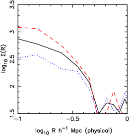
Figure 16: The mean surface density of the groups (arbitrary units) versus radius. The ratio of red (dashed) to blue (dotted) galaxies increases towards the centre. The solid line is for all galaxies.

The average group surface density profile, $\Sigma(R)$, Figure 16, is based on about 200 galaxies. The mean projected slope between $\log{R}=-1$ and $\log{R}=-0.5$ of all the galaxies is almost exactly $d\log(\Sigma)/d\log(r)=-1$, which deprojects to $\mathchar 28951\relax\propto r^{-2}$ of the isothermal sphere. The red galaxies are more concentrated than the blue galaxies in these groups, with small differences in the luminosity function from the field. The projected velocity dispersion profile, Figure 17, of both the full sample is consistent with no radial variation in the mass to total light ratio. However the blue galaxies have significantly higher velocity dispersions than the red galaxies with an indication of a drop with radius. This is quite distinct from the pairwise velocities, in which blue galaxies have significantly lower velocities than red galaxies. This helps one to understand why the virial masses given by blue galaxies are about 50% higher than the full sample. Red galaxies give virial masses that are 98% of the full sample result. We take these surface density and velocity dispersion profiles as tentative evidence that the full galaxy distribution and the mass distribution in groups are similar. Within groups, blue galaxies are “anti-biased” with respect to the red galaxies and likely the mass as well.

Although these results are both preliminary and clearly subject to statistical uncertainties, they would support the notion that these groups are in many ways dynamically similar to rich clusters although they do not have such extreme population differences as rich clusters and the field. These issues are a major area of investigation in the CNOC2 survey.

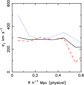
Figure 17: The projected velocity dispersion versus radius in the groups. Blue galaxies (dotted) have systematically higher velocity dispersions than the red galaxies (dashed), which are similar to the full sample (solid).

8 Ultra-Large Scale Power

Measuring the power spectrum on scales of 100-500$h^{-1}$ Mpc, roughly the scale of the “first Doppler peak” in the CMB fluctuation spectrum, requires a survey that covers an appreciable fraction of the visible universe. Pencil beam surveys do just that, but only in one dimension which leads to the problem of aliasing in of shorter scale power into the derived 1D power spectrum, $P_{1}(k)$. In view of previous results ([Broadhurst et al. 1990]) and the fundamental interest in this statistic we measure the one dimensional power spectrum from the CNOC2 data and compare it to various simple models.

The one dimensional power spectrum $P_{1}(k)=|N^{-1}\sum_{i=1}^{N}\exp{[ikx_{i}]}|^{2}$ (unweighted) is shown as the upper irregular line in Figure 18. At very large $k_{z}$ this tends to $1/N$ where $N\simeq 1500$ in each of our patches. The observed 1D spectrum requires some care in interpretation since the 1D power at a large wavenumber is an integral over the entire 3D spectrum ([Kaiser & Peacock 1991]) whose analysis we follow here. The 1D power spectrum of the smooth $n(z)$ is the $W(k_{z})$ window function and is shown as the lower irregular line. Clearly the power at $k_{z}<0.01{h^{-1}\,\hbox{Mpc}}^{-1}$ is completely dominated by the smooth distribution of the data. At shorter wavelengths, $\mathchar 28949\relax<600{h^{-1}\,\hbox{Mpc}}$, the observed power spectrum is a result of real structure.

Figure 18: The one dimensional power spectrum and related quantities. The lower irregular line is the power spectrum of the smooth $n(z)$ distribution. The upper irregular line is the power spectrum of the observed redshifts averaged over the two fields. The upper smooth line is for $(r_{0}/r)^{1.7}$, with $r_{0}=4.2{h^{-1}\,\hbox{Mpc}}$ (co-moving) which is modified with a Gaussian peculiar velocity distribution of 300  km s^-1 and then the power correlation truncated at 50 and 100 $h^{-1}$ Mpc.

The null hypothesis is that the 1D power spectrum is simply the power spectrum of the real space correlation function, $(r_{0}/r)^{\mathchar 28941\relax}$, as projected into these observations. The 3D power spectrum is $P(k)=4\mathchar 28953\relax k^{-3}(kr_{0})^{\mathchar 28941\relax}\Gamma(2-\mathchar 28941\relax)\sin{[(2-\mathchar 28941\relax)\mathchar 28953\relax/2]}$. To derive the window function on the sky we do a Monte Carlo evaluation of $W(k_{x},k_{y})$ by randomly populating the sky patches and transforming. To evaluate the predicted 1D spectrum we approximate the $z$ window function as $2\mathchar 28953\relax/L_{z}$, and integrate the product of the sky window function with $P(k)$. The results are displayed in Figure 18, where we have added a constant shot noise of $1/N$. The unaltered spectrum does a very poor job of describing the observed spectrum. The two necessary modifications are to add a random peculiar velocity and a long wavelength decline in power. The random velocities are modeled using a Gaussian (clearly not a very good description of these data) at 300  km s^-1. Any CDM type spectrum rolls over in the 30-100 $h^{-1}$ Mpc range. We simply truncate the input power spectrum at 50 and 100 $h^{-1}$ Mpc to produce the plots displayed. We can conclude that the universe is not a fractal with a fixed clustering dimension to all scales, and is otherwise consistent (at the current statistical level) with the known large scale clustering power spectrum ([Lin et al. 1996b]).

9 Preliminary Conclusions

The CNOC2 sample spans a range of redshifts which has dramatic galaxy evolution but in which detailed studies are readily performed. Our preliminary conclusions are discussed below.

Galaxy evolution is confirmed to be strongly differential with the blue, low mass galaxies changing significantly in their visible numbers. We find luminosity functions similar in their overall features to previous studies ([Lilly et al. 1995, Ellis et al. 1996]) but with smaller statistical errors. The evolution of the early and intermediate SED types is well described as a pure luminosity evolution. In contrast, the late type SED population is described as nearly pure density evolution. It should be noted that the density evolution could be at least partly in the form of varying duty cycle of star formation.

The correlation of galaxies above $M_{\ast}+0.3$ mag is about 60% higher than those below, with a mean sample luminosity difference of 1.4 mag. This is consistent with the expected intrinsic correlation differences of dark matter halos of different mass scales. Having a cleaner mass cut (from the SED model fits) and more data to trace the evolution of this effect will allow a more confident conclusion.

Blue galaxies are about 50% less correlated than red galaxies on scales beyond about 0.3$h^{-1}$ Mpc. On shorter scales blue galaxies have a break in their correlation function and become about a factor of three less correlated than red galaxies. On large scales the difference is about what one would expect from the smaller average masses of the blue galaxies. Because the $\mathchar 28952\relax(r)$ break occurs at about the average virialization scale it suggests that the blue-red difference is an active environmental effect. Dynamically virialization occurs where tidal stripping begins to remove the dark halos and their contents from infalling galaxies.

Figure 19: The evolution of the proper density of galaxies around galaxies, with the $M_{R}^{k,e}$ LCRS and CNOC2 sample at low redshift and the Giavalisco et al. (1998) inversion at high redshift.

A primary result is that we find that the correlation evolution of galaxies brighter than $M_{R}=-20$, where $M_{\ast}=-20.3$ mag, are well described with $\mathchar 28952\relax(r)=(r_{0}/r)^{\mathchar 28941\relax}(1+z)^{-3-\mathchar 28943\relax}$, where $r_{0}=5.15\pm 0.15{h^{-1}\,\hbox{Mpc}}$ (proper co-ordinates), $\mathchar 28941\relax=1.77\pm 0.05$, and $\mathchar 28943\relax=-0.6\pm 0.4$. That is, the physical density of galaxies around galaxies is declining slightly with redshift. Figure 19 shows that the extrapolation of our rate of clustering evolution passes smoothly through the inversion of the angular correlation of the high luminosity $z\simeq 3$ “Steidel objects” ([Giavalisco et al. 1998], but note [Adelberger et al. 1998]). We note that the association of our population of objects with theirs is not secure.

The measured $\mathchar 28943\relax$ is completely incompatible with the $\mathchar 28943\relax\simeq 1$ expected for the mass field in an $\Omega_{M}=1$ universe. The result is about half way between mass clustering in a low density universe and the clustering evolution of the relatively high density cores of dark matter halos ([Colin, Carlberg & Couchman 1997]). In general an $\mathchar 28943\relax<0$ implies that bias is changing with redshift, although in a low $\Omega_{M}$ model this is a very slow function of redshift. An interpretation of the slow drop in proper density, within the context of n-body simulations, is that it is due to merging of galaxies in high density regions. Taking the result at face value, this means that about $35\pm 20\%$ of all the high luminosity galaxies will have merged since redshift one. If the time scale for merging is 1 Gyr, then the merging fraction will be about $4\pm 3\%$, on average, close to the estimates of Patton et al. (1997).

The pairwise velocity dispersions of the luminous galaxies do not detectably evolve between $z=0.05$ and $z=0.4$, remaining constant at about 350  km s^-1 (for our chosen estimator). The Cosmic Virial Theorem gives $Q\Omega_{M}/b=0.11\pm 0.04$, where $Q$ is the three point correlation parameter. The three point parameter will be estimated from these data, with the expectation that $Q\simeq 1$ from low redshift results.

Galaxy groups with line-of-sight velocity dispersions between 100 and 400  km s^-1 are found, with numbers declining with increasing $\mathchar 28955\relax_{1}$, very roughly as expected from Press-Schechter theory. The virial M/L values may drop at small $\mathchar 28955\relax_{1}$ (perhaps due to dynamical inspiral) with the higher velocity dispersion objects having M/L values consistent with the population adjusted values of rich clusters. The mean M/L is about 35% below rich clusters. The groups are consistent with the total galaxy light being distributed like the mass. The groups have a weak population gradient, becoming redder from the “edge” of the mean group toward its centre. We tentatively associate the break in the $\mathchar 28952\relax(r)$ of blue galaxies with this behaviour of groups. The groups, averaged together, indicate $\Omega_{M}=0.15\pm 0.05$.

The one-dimensional power spectrum of our pencil beams requires that the the observed power law correlation at scales of less than 10$h^{-1}$ Mpc must have a turnover at about 100$h^{-1}$ Mpc, which is of course expected in CDM-like theories and indicated by observations of large scale clustering at low redshift.

We set out to test theories of galaxy and structure evolution by measuring the evolution. In spite of the dramatic changes in the numbers of lower luminosity, blue galaxies, the systems of higher luminosity that dominate the stellar mass of the universe appear to be nearly a static population, having only a small change in the density of similar galaxies around them and little star formation over our redshift range.

These preliminary analyses are based on 1/2 of the eventual data for which we complete observations in May 1998. The results are likely to change somewhat (especially as other estimators are implemented and systematic errors detected and eliminated). Perhaps the primary conclusion to be drawn is that the CNOC2 dataset will be a rich sample for the study of cosmology, large scale structure and galaxy evolution.

References

- Adelberger et al. 1998 Adelberger, K., Steidel, C., Giavalisco, M., Dickinson, M., Pettini, M., & Kellogg, M. 1998, ApjL in press (astro-ph/9804236)
- Bean et al. 1983 Bean, A. J., Ellis, R. S., Shanks, T., Efstathiou, G., & Peterson, B. A. 1983, MNRAS, 205, 605
- Bruzual & Charlot 1996 Bruzual, A. G. & Charlot, S. 1996, in preparation
- Broadhurst et al. 1990 Broadhurst, T. J., Ellis, R. S., Koo, D. C. & Szalay, A. S. 1990, Nature 343, 726
- Carlberg 1994 Carlberg, R. G. 1994, ApJ, 433, 468
- Carlberg et al. 1996 Carlberg, R. G., Yee, H. K. C., Ellingson, E., Abraham, R., Gravel, P., Morris, S. M, & Pritchet, C. J. 1996, ApJ, 462, 32
- Carlberg, Yee & Ellingson 1997 Carlberg, R. G., Yee, H. K. C., & Ellingson, E. 1997, ApJ, 478, 462
- Carlberg, Cowie, Songaila & Hu 1997 Carlberg, R. G., Cowie, L., L., Songaila, A., & Hu, E. M. 1997, ApJ, 483, 538
- Coleman, Wu & Weedman 1980 Coleman, G. D., Wu, C.-C., & Weedman, D. W. 1980, ApJS, 43, 393
- Colin, Carlberg & Couchman 1997 Colin, P., Carlberg, R. G., & Couchman, H. M. P. 1997, ApJ, 390, 1
- Croft, Dalton & Efstathiou 1998 Croft, R. A. C., Dalton, G. B., & Efstathiou, G. 1998, MNRAS submitted (astro-ph/9801254)
- Davis & Peebles 1983 Davis, M. & Peebles, P. J. E. 1983, ApJ, 267, 465
- Ellis et al. 1996 Ellis, R. S., Colless, M., Broadhurst, T., Heyl, J. & Glazebrook, K 1996, MNRAS 280, 235
- Giavalisco et al. 1998 Giavalisco, M., Steidel, C. C., Adelberger, K. L., Dickinson, M. E., Pettini, M. & Kellogg, M. 1998, ApJ, in press (astro-ph/9802318)
- Ghigna et al. 1998 Ghigna, S., Moore, B., Governato, F., Lake, G., Quinn, T., Stadel, J. 1998, MNRAS submitted (astro-ph/9801192)
- Giovanelli & Haynes 1991 Giovanelli, R. & Haynes, M. P 1991, ARA&A 29, 499
- Guzzo et al. 1997 Guzzo, L., Strauss, M. A., Fisher, K. B., Giovanelli, R., & Haynes, M. P. 1997, ApJ, 489, 37
- Jenkins et al. 1997 Jenkins, A., Frenk, C. S., Pearce, F. R., Thomas, P. A., Colberg, J. M., White, S. D. M., Couchman, H. M. P., Peacock, J. A., Efstathiou, G. & Nelson, A. H. 1997, preprint (astro-ph/9709010)
- Kaiser & Peacock 1991 Kaiser, N. & Peacock, J. 1991, ApJ, 379, 482
- LeFèvre et al. 1994 LeFèvre, O., Crampton, D., Felenbok, P., & Monnet, G. 1994, A&A, 282, 340
- LeFèvre et al. 1996 LeFèvre, O, Hudon, D., Lilly, S. J. Crampton, D., Hammer, F. & Tresse, L. 1996, ApJ, 461, 534
- Lilly et al. 1995 Lilly, S. J., Tresser, L., Hammer, F., Crampton, D. & LeFèvre, O. 1995, ApJ, 455, 108
- Lin et al. 1996a Lin, H., Kirshner, R. P., Schectman, S. A., Landy, S. D., Oemler, A., Tucker, D. L., & Schechter, P. L. 1996, ApJ, 464, 60
- Lin et al. 1996b Lin, H., Kirshner, R. P., Schectman, S. A., Landy, S. D., Oemler, A., Tucker, D. L., & Schechter, P. L. 1996, ApJ, 471, 617
- Lin et al. 1998a Lin, H., Yee, H. K. C., Carlberg, R. G., Morris, S. L., et al. 1998a, to be submitted to ApJ
- Lin et al. 1998b Lin, H., Yee, H. K. C., Carlberg, R. G., Morris, S. L., et al. 1998b, to be submitted to ApJ
- Loveday et al. 1995 Loveday, J., Maddox, S. J., Efstathiou, G. & Peterson, B. A. 1995, ApJ, 442, 457
- Patton et al. 1997 Patton, D., Pritchet, C. J., Yee, H. K. C., Ellingson, E., & Carlberg, R. G., 1997, ApJ, 475, 29
- Peebles 1980 Peebles, P. J. E. 1980, “Large Scale Structure of the Universe”, Princeton University Press, Princeton
- Press & Schechter 1974 Press, W. H. & Schechter, P. 1974, ApJ, 187, 425
- Shepherd et al. 1996 Shepherd, C. W., Carlberg, R. G., Yee, H. K. C. & Ellingson, E. 1996, ApJ, 479, 82
- Schectman et al. 1996 Schectman, S. A., Landy, S. D., Oemler, A., Tucker, D. L, Lin, H., Kirshner, R. P. & Schechter, P. L. 1996, ApJ, 470, 172
- Yee 1991 Yee, H. K. C. 1991, PASP 103, 396
- Zaritsky & White 1994 Zaritsky, D. & White, S. D. M. 1994, ApJ, 435, 599