Comment on the paper “The ESO Slice Project galaxy redshift survey: V. Evidence for a D=3 sample dimensionality”

Abstract

In a recent analysis of number counts in the ESP survey Scaramella et al. (1998) claim to find evidence for a cross-over to homogeneity at large scales, and against a fractal behaviour with dimension $D\approx 2$. In this comment we note firstly that, if such a cross-over exists as described by the authors, the scale characterizing it is $\sim 100\div 300h^{-1}Mpc$. This invalidates the “standard” analysis of the same catalogue given elsewhere by the authors which results in a “correlation length” of only $r_{0}=4h^{-1}Mpc$. Furthermore we show that the evidences for a cross-over to homogeneity rely on the choice of cosmological model, and most crucially on the so called K corrections. We show that the $D\approx 3$ behaviour seen in the K-corrected data of Scaramella et al. is in fact unstable, increasing systematically towards $D=4$ as a function of the absolute magnitude limit. This behaviour can be quantitatively explained as the effect of K-correction in the relevant range of red-shift ($z\sim 0.1\div 0.3$). A more consistent interpretation of the number counts is that $D$ is in the range $2\div 2.5$, depending on the cosmological model, consistent with the continuation of the fractal $D\approx 2$ behaviour observed at scales up to $\sim 100h^{-1}Mpc$. This implies a smaller K-correction. Given, however, the uncertainty in the effect of intrinsic fluctuations on the number counts statistic, and its sensitivity on these large scales to the uncertain K corrections, we conclude that it is premature to put a definitive constraint on the galaxy distribution using the ESP data alone.

1 Introduction

In a recent paper Scaramella et al.(1998; S&C ) have applied the same statistical analysis to two deep surveys of large scale structure -the ESP galaxy survey, and the Abell and ACO survey of clusters - as performed by three of us and reported in Sylos Labini et al.(1998; Paper 1). Despite the adoption of the same method, they have reached very different conclusions: That there is no evidence for a scale invariant distribution of galaxies with dimensionality $D\approx 2$, as argued in Paper 1, and that their results favour the “canonical” value of $D=3$ (corresponding to a homogeneous universe). In this comment we will concentrate on a few specific points, referring the reader to Paper 1 for detailed discussion of various points on which we have nothing new to add. Firstly we clarify what the claims of Paper 1 for a fractal distribution of galaxies actually are, in particular the strength of the statistical evidence on different scales, as the discussion given in S&C is unclear on this point. We then turn to a detailed discussion of the analysis of the ESP data, discussing the results and different interpretations of Paper 1 and S&C. Our main substantial result is the demonstration that the $D=3$ behaviour which appears in the data when K corrected as prescribed in S&C is in fact unstable, with $D$ increasing systematically to substantially larger values as a function of the depth of the volume limited sample. Quantitatively this behaviour can be explained as the effect of a large K correction applied to an underlying galaxy distribution with fractal dimension $D\approx 2$. We only briefly comment on the analysis of the Abell and ACO cluster catalogues as a full discussion of the relevant issues is given in Paper 1.

2 Statistical Methods

The assumption of homogeneity in the distribution of matter lies at the heart of the Big Bang cosmology. The nature of the evidence, if any, for this assumption has, however, been the subject of considerable controversy (Davis 1997, Pietronero et al., 1997). A central point made by one of us (LP, Pietronero 1987) has been that the standard methods of analysis of galaxy red-shift catalogues, which provide the most direct probe of the (luminous) matter distribution, actually assume homogeneity implicitly. An alternative analysis has been proposed using statistical methods which do not make this assumption, and are appropriate for characterizing the properties of regular as well as irregular distributions. Essentially this analysis makes use of a very simple statistic, the conditional average density, defined as

$$\Gamma(r)=\left\langle\frac{1}{S(r)}\frac{dN(<r)}{dr}\right\rangle$$ (1)

where $dN(<r)$ is the number of points in a shell of radius $dr$ at distance $r$ from an occupied point and $S(r)dr$ is the volume of the shell. Note that in Eq.1 there is an average over all the occupied points contained in the sample. If the distribution is scale invariant with fractal dimension $D$ we have

$$\Gamma(r)\sim r^{-\gamma}\;$$ (2)

where $\gamma=3-D$.

The problems of the standard analysis can easily be seen from the fact that, for the case of a fractal distribution the standard “correlation function” $\xi(r)$ in a spherical sample of radius $R_{s}$, is given by

$$\xi(r)=\frac{3-\gamma}{3}\left(\frac{r}{R_{s}}\right)^{-\gamma}-1\;.$$ (3)

Hence for a fractal structure the “correlation length” $r_{0}$ (defined by $\xi(r_{0})=1$), is not a scale characterizing any intrinsic property of the distribution, but just a scale related to the size of the sample. If, on the other hand, the distribution is fractal up to some scale $\lambda_{0}$ and homogeneous beyond this scale, it is simple to show that, if $\lambda_{0}<R_{s}$, i.e. the crossover to homogeneity is well inside the sample size,

$$r_{0}=\lambda_{0}\cdot 2^{-\frac{1}{\gamma}}\;.$$ (4)

The correlation length does in this case have a real physical meaning (when measured in samples larger than $\lambda_{0}$), being related in a simple way to the scale characterizing homogeneity. In the case $D=2$ we have $r_{0}=\lambda_{0}/2$ .

3 The debate on the fractal universe

The most popular point of view is that given, for example, by Peebles (1993) and Davis (1997) according to which the homogeneity scale has already been well established by means of different observations. Peebles (1993) argues that the homogeneity of the matter distribution is indicated by the uniformity of galaxy angular catalogs, the number counts of galaxy as a function of apparent magnitude and the so-called “rescaling” of the amplitude of the angular correlation function. In particular a correlation length $r_{0}\approx 5h^{-1}Mpc$ is taken to be a real physical scale characterizing the departure from homogeneity. Increase in this quantity with depth of sample is ascribed to the so-called “luminosity bias” (Davis et al., 1988; see also Benoist et al., 1996). In complete disagreement with these claims is the direct analysis of all available galaxy catalogues reported in Paper 1, using the conditional average density $\Gamma(r)$. Up to the deepest scales for which such an analysis can be carried out for available catalogues clear evidence for fractal behaviour with $D\approx 2$ has been found. No evidence for a cross-over to homogeneity at the scales required to make the standard analysis meaningful is found, nor indeed any evidence for such a cross-over at scales within the range of current catalogues with robust statistics, which place a lower bound on $\lambda_{0}$ of approximately $100h^{-1}Mpc$.

This length scale for these statements is fixed by the maximum radius of a sphere which can be fitted inside the sample volume of the corresponding surveys, since the statistic $\Gamma(r)$ can only be computed up to such a distance. To extract information from surveys about correlations at length scales greater than this, one needs to consider other statistics. The most simple one is the radial count $N(<r)$ from the origin in whatever solid angle is covered by the survey. Depending on the survey geometry the difference between the length scales to which we can calculate $\Gamma(r)$ and $N(<r)$ varies greatly. The number count from the origin is obviously a much less powerful statistic since it doesn’t involve the average. It is intrinsically a more fluctuating quantity. Such fluctuations are, however, about the average behaviour and, by sampling a sufficiently large range of scale, one should be able to recover the average behaviour of the number count $\sim r^{D}$. What one means by “sufficiently large range of scale” depends strongly on the underlying nature of the fluctuations. In particular (see section 6.1 of Paper 1) the cases of a homogeneous distribution with Poissonian type fluctuations and a fractal structure with scale invariant fluctuations are quite different. In the former case one predicts a very rapid approach to perfect $D=3$ behaviour at a few times the scale characterizing the fluctuations; in the latter $N(<r)$ has intrinsic fluctuations on all scales (which average out in $\Gamma(r)$), in addition to the statistical sampling Poisson noise in $N(<r)$ which dominates up to a scale which depends on the sample (on the number of points, and therefore on the solid angle of the survey).

4 Analysis of the ESP redhsift survey

We now turn to the ESP survey, which is a very deep survey extending to red-shifts $z\sim 0.3$ in a very narrow solid angle $\Omega\approx 0.006\;sr$. Because of this geometry the analysis with $\Gamma(r)$ only extends to $R_{s}\approx 10\div 12h^{-1}Mpc$; in this regime it shows a clear $D\approx 2$ behaviour consistent with the other surveys analyzed in Paper 1. With the radial counts from the origin $N(<r)$, however, the analysis can extend to distances almost two orders of magnitude greater. The results of the latter analysis can be summarized as follows:

$\bullet$ Up to a scale of $\sim$ 300 $h^{-1}Mpc$ the number counts are highly fluctuating;

$\bullet$ Beyond this scale the counts can be well fitted by a fairly stable average behaviour $N(<r)\sim r^{D}$.

The value obtained for the dimension of the number count $D$ in this range depends (i) on the assumptions about the cosmology and (ii) on the so-called K corrections. The uncorrected data (i.e. with the euclidean distance relation and without K corrections) gives a slope of $D\approx 2$, while both corrections lead to an increase in the slope. In particular S&C apply the corrections in a way which produces values $D\approx 3$ which they argue to reflect the true behaviour of the galaxy distribution.

4.1 The fluctuating regime: $r\mathrel{\hbox to0.0pt{\lower 3.0pt\hbox{$\mathchar 536\relax$}\hss}\raise 2.0pt\hbox{$\mathchar 316\relax$}}300h^{-1}Mpc$

Consider first what conclusions may be drawn from the fluctuating regime. If the universe is homogeneous on large scales, the data clearly show that the scale characterizing such homogeneity is at least $\sim 100\div 300h^{-1}Mpc$. The implication from our discussion above is that any standard analysis using the correlation function is inappropriate for characterizing the properties of the fluctuations. In particular the authors claim in various papers (see e.g. Guzzo, 1997) that in the ESP galaxy sample, $r_{0}\approx 4h^{-1}Mpc$. The origin of this length scale can also be inferred from the discussion above: In a fractal distribution (with $D=2$) we see from (3) that $r_{0}\approx R_{s}/3$, and as noted above $R_{s}\approx 10\div 12$ in the ESP survey. It is related not to a physical property of the galaxy distribution but to the specific geometry of the survey it has been determined from. The more general implication of this observation of large fluctuations up to 300 $h^{-1}Mpc$ for all standard analyses of existing catalogues is also clear . If, on the other hand, the true underlying behaviour is fractal, the transition from a highly fluctuating to a more stable behaviour can be understood as the transition between large statistical fluctuations and much smaller scale-invariant intrinsic fluctuations. In Paper 1 it is shown how, using the dimension and normalization of the radial density from the analysis of the other surveys analyzed with the $\Gamma(r)$ statistic, one obtains a simple estimate for this scale in ESP which agrees with the observation that it is $\sim$ 300 $h^{-1}Mpc$. The observed fluctuating regime is therefore consistent with the continuation of the fractal behaviour seen at smaller scales.

4.2 The large scale regime: $r\mathrel{\hbox to0.0pt{\lower 3.0pt\hbox{$\mathchar 536\relax$}\hss}\raise 2.0pt\hbox{$\mathchar 318\relax$}}300h^{-1}Mpc$

Now let us move onto the conclusions which can be drawn from the smoother regime at larger scales. In Paper 1 it was noted that from $\sim 300h^{-1}Mpc$ the number counts show very approximately a dimension $D\approx 2$, and therefore provide weak evidence for the continuation of the behaviour seen at smaller scales. Different redshift-distance relations and some typical K corrections were also applied to the data, but, given the uncertainty in their determination, they were not interpreted as sufficiently reliable to change an already statistically weak conclusion. In particular, for example, detailed fits to different VL samples were not performed. In S&C the authors have looked at the precise effect which certain corrections can have on the data in the regime beyond $300h^{-1}Mpc$ in much greater detail, and drawn the strong conclusion that the $D\approx 2$ behaviour is ruled out and $D=3$ behaviour clearly favoured.

The difference of interpretation centres on the K corrections, and the strength of any conclusion on the confidence with which they can be made. We will now see that some checking shows that the K corrections as they have been applied to obtain this result are actually inconsistent with the conclusion of an underlying $D=3$ dimensionality.

4.3 Volume Limited (VL) samples and the effect of K-correction

In order to construct VL catalogues we need to determine the absolute magnitude $M$ of a galaxy at redshift $z$ from its observed apparent magnitude $m$, and it is here that the K correction enters:

$$M=m-5log(d_{L})-25-K(z)$$ (5)

Here the luminosity distance $d_{L}=r(1+z)$ in Friedmann-Robertson-Walker (FRW) models where $r$ is the comoving distance, and $d_{L}=(c/H_{o})z$ in the euclidean case. The K correction corrects for the fact that when a galaxy is red-shifted we observe it in a redder part of its spectrum where it may be brighter or fainter. It can in principle be determined from observations of the spectral properties of galaxies, and has been calculated for various galaxy types as a function of red-shift (e.g. Fukugita et al., 1995). When applying them to a red-shift survey like ESP, we need to make various assumptions since we lack information about various factors (galaxy types, spectral information etc. as a function of red-shift and magnitude).

It is not difficult to understand how K corrections affect the number counts systematically. The number count in a volume limited sample corresponding to an absolute magnitude limit $M_{lim}$ can be written schematically as

$$N(<R)=\int_{0}^{R}\rho(r)d^{3}r\int_{-\infty}^{M_{lim}}\phi(M,r)dM$$ (6)

where $\rho(r)$ is the real galaxy density, and $\phi(M,r)$ the appropriately normalized luminosity function (LF) in the radial shell at $r$. If the latter integral is independent of the spatial coordinate (i.e. if the fraction of galaxies brighter than a given absolute magnitude is independent of $r$), it is just an overall normalization and the exponent of the number counts in the VL sample show the behaviour of the true number count, with $N(<R)\sim R^{D}$ corresponding to the average behaviour $\rho\sim r^{D-3}$ as we have assumed. What we do when we apply K corrections or other red-shift dependent alterations to the relation (5) is effectively to change the LF $\phi(M,r)$. Using an incorrect relation will induce $r$ dependence in this function, which in turn will distort the relation between radial dependence of the number counts and the density.

When one applies a K correction and observes a significant change in the number counts, there are thus two possible interpretations - that one has applied the physical correction required to recover the underlying behaviour for the galaxy number density, or that one has distorted the LF to produce a radial dependence unrelated to the underlying density. How can one check which interpretation is correct? Consider the effect of applying a too large K correction. To a good approximation the net effect is a linear shift in the magnitude $M$ with red-shift, so that $M\rightarrow M-kz$. The second integral in (6) can in this case be written

$$\int_{-\infty}^{M_{lim}}\phi_{p}(M+kz)dM=\int_{-\infty}^{M_{lim}+kz}\phi_{p}(M)dM$$ (7)

where $\phi_{p}$ denotes the physical, r-independent LF. This is a function whose shape is well known to be fitted by a very flat power-law with an exponential cut-off at the bright end. If the upper cut-off of the integral is in the former range, one can see from (6), taking $z\sim r$, that the number count picks up an additional contribution going as $R^{D+1}$, so that we expect the slope to increase by one at some sufficiently large scale. As we go to the brighter end of the luminosity function, where it turns over, the fractional number of galaxies being added by the correction is even greater and we expect to see a growing effect on the slope with depth of sample. To illustrate the effect quantitatively we have computed the integral (6) numerically for a distribution $\rho(r)$ which has an average $D=2$ behaviour in euclidean co-ordinates, taking $\phi(M,r)=\phi_{p}(M+K(z))$, where $\phi_{p}(M)$ is the LF for the ESP survey given in Zucca et al.(1997), and $K(z)$ the average K correction used in S&C.

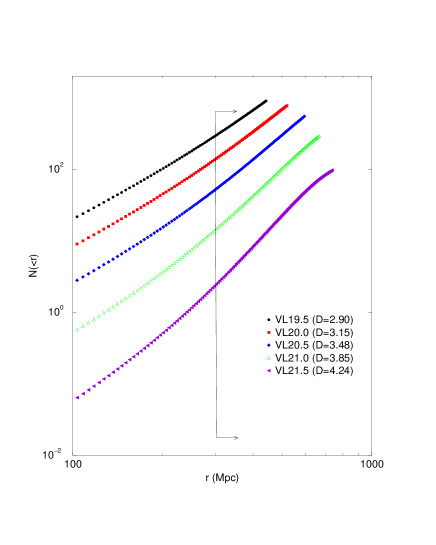
Fig. 1.: A plot of average number counts in a survey with the LF of the ESP survey ($\alpha=1.2$ and $M^{*}=-19.6$), if the underlying distribution has fractal dimension $D=2$ in euclidean coordinates, with a shift to the LF corresponding to the K correction applied by S&C. The different VL samples are labelled according to the cut in absolute magnitude (i.e. VL20.5 corresponds to a cut at $M=-20.5$). The distance $r$ is that for the flat FRW cosmology used by S&C ($q_{o}=0.5$). At scales $r\mathrel{\hbox to0.0pt{\lower 3.0pt\hbox{$\mathchar 536\relax$}\hss}\raise 2.0pt\hbox{$\mathchar 318\relax$}}300h^{-1}Mpc$ we see that the effect is to produce an exponent $D\approx 3$, increasing systematically to larger values as we go to deeper VL samples with an absolute magnitude cut $M\mathrel{\hbox to0.0pt{\lower 3.0pt\hbox{$\mathchar 536\relax$}\hss}\raise 2.0pt\hbox{$\mathchar 318\relax$}}M^{*}$. The fit with a power law function has been done in the region to the right of the arrow.

The results plotted in Fig. 1 show that, on the scales over which the ESP data are analysed, we should be able to clearly distinguish the case of a spurious K correction from the case of a real underlying $D=3$ behaviour, which should be relatively stable as a function of the absolute magnitude limit of the VL sample. In Figure 2 of their paper S&C show the number counts for a few VL samples, and conclude that there is evidence for a real sample slope of $D=3$, the variation being ascribed to random errors. In Fig. 2 we show precisely the same figure with additional VL samples at greater depth, which have been omitted by S&C.

Fig. 2.: The figure corresponds to Fig.2 of S&C ($q_{o}=0.5$ with exactly the K correction given in Zucca et al.1997), but including deeper VL samples. For each VL sample it is reported the limiting redshift and absolute magnitude. The systematic growth of the exponent of the number counts as a function of the absolute magnitude limit of the sample is clearly seen. The fit with a power law function has been done in the region to the rigth of the arrow. The value of the fractal dimension $D$ for each VL sample is reported in the label; in brakets it is shown the error on the fractal dimension estimated with 40 boostrap resamplig.

The conclusions one can draw from these two figures are clear: The $D\approx 3$ behaviour observed by S&C in their K corrected data is clearly not stable as would be the case if it represented the real underlying behaviour of the density. On the contrary, as we see from Fig. 1, the “corrected” data are in fact clearly better interpreted as indicating an underlying distribution with $D\approx 2$ which has been subjected to a too large K correction in the relevant range of red-shift $z\sim 0.1-0.3$.

4.4 Dependence on the cosmological model

What about the dependence on cosmological model? Can we find a more consistent $D=3$ fit with the same K corrections by changing the deceleration parameter $q_{o}$? The effect of changing cosmological model is two-fold: (i) It changes the relation between red-shift and the comoving distance in which we should see the homogeneity, and (ii) it changes the absolute magnitude through relation (5). The effect of the former is relatively minor for the red-shifts we are considering here, increasing the slope by at most about $0.2$. The latter effect has the same form as that of the K-correction since, at linear order in red-shift, $d_{L}=d_{E}[1+\frac{1}{2}(1-q_{o})z+...]$ where $d_{E}=(c/H_{o})z$ is the euclidean distance, and therefore from (5) we see that it is equivalent to an effective linear K correction with $k_{eff}=5(1-q_{o})/2\ln 10$. So, taking any FRW model with a sub-critical matter density essentially adds an even larger K correction of the type taken by S&C and leads to steeper slopes with an even more unstable behaviour as a function of depth. For example, we show the results in Fig. 3 for a currently popular critical FRW model with a cosmological constant $\Omega_{\Lambda}=0.7$ (giving $q_{o}=-0.55$)

Fig. 3.: Same as Figure 2 but with $q_{0}=-0.55$

Adopting different FRW cosmological models from the one used by S&C in their analysis produces results even more inconsistent with homogeneity. In contrast with the conclusion of S&C that the $D\approx 2$ result of Paper 1 is only tenable by “both unphysically ignoring the galaxy K-correction and using euclidean rather than FRW cosmological distances”, we conclude therefore that the alternative $D=3$ result is arrived at only by applying an unphysical K correction and taking a specific FRW cosmology.

The strong dependence on the chosen FRW cosmology is interesting by itself. Without any K corrections the $q_{o}=0.5$ cosmology gives slopes of $\approx 2.4$, while for the $q_{o}=-0.55$ case we get values from $2.5$ to $2.8$ as we go to deeper samples. If we had confidence in applying the K correction, very strong conclusions could be drawn about these models. It is perhaps interesting to note that any approximately linear K correction will not produce a stable dimension near $D=3$ for this data in these models. Clearly the physical K correction in this range of red-shift must be a very non-trivial function quite different from that used by S&C if the ESP data arises from an underlying homogeneous distribution. In the absence of a clearly consistent and well understood way of applying such corrections, it makes little sense to draw conclusions which depend so strongly on them. By contrast the interpretation of a continuation of fractal behaviour with $D\approx 2$ (and a relatively unimportant role for K corrections) is consistent, supported also by the behaviour seen in the fluctuating regime. With a smaller linear K correction with k=1, for example, we find a stable slope in euclidean coordinates around $D=2.2$.

5 Discussion

Besides consistency requirements of this type, can we determine more directly what the physical K corrections are (in the absence of direct measurements of the necessary spectral information)? Clearly this is a general question which is not simply of relevance to ESP, but to the analysis of any survey which stretches to such scales. In particular, if there is a cross-over to homogeneity, we have seen that it is at least at scales of hundreds of megaparsecs, and therefore these corrections will be of importance in the analysis of any forthcoming survey to search for evidence for homogeneous or fractal behaviour. The approach of S&C takes the K corrections from other sources and applies them with various assumptions to their survey. We have seen that, at least for this case, a simple check shows that this procedure gives incosistent results. Can we see this more directly? As we discussed above, the physical effect underlying the K correction produces a red-shift dependent distortion of the (uncorrected) LF. By looking at the (uncorrected) LF in different slices of the survey we should, in principle, be able to see its effect. Furthermore, if we are applying K corrections to the data in the appropriate way, we should be able to see them “undo” such distortion. For the ESP survey we have broken up various VL limited samples into ‘nearby’ and ‘distant’ slices and looked at the LF in the uncorrected and ‘corrected’ catalogues. This analysis shows that the uncorrected catalogue shows good agreement between the LF in the two samples at different depth, compared to samples in the catalogue ‘corrected’ as in S&C, in which we see clear evidence for a too large K-correction causing an unphysical distortion of the LF. However, because the statistics are weak, we cannot derive any strong statement about what the real K correction effect is. An analysis of the effect of K corrections on the LF should however provide very useful consistency checks in the analysis of the much larger forthcoming redshift surveys.

6 Conclusion

More generally we emphasize that the degree of uncertainty in the results here is related to the fact that we are using only the radial counts from the origin, which are extremely sensitive to these effects which produce systematic distortions relative to this origin. These effects will be much less with the full correlation function, which averages over points. In a forthcoming work we will discuss in more detail the effect of different corrections on the various statistics. To draw strong statistical conclusions about the distribution at large scales like those which have been possible at moderate scales (up to $\sim$ 100$h^{-1}Mpc$) we will probably have to await the completion of the much larger surveys in progress.

Finally a brief comment on the cluster distributions, of which a detailed discussion is given in Paper 1. An analysis with the conditional average density $\Gamma(r)$ is possible up to $\sim 80h^{-1}Mpc$, and shows clearly defined fractal properties with $D\approx 2$. The number counts from the origin show a quite fluctuating behaviour up to about $\sim 100h^{-1}Mpc$, and clear incompleteness at scales considerably larger than this (evidenced by a steep decrease in the number counts). The identification of a range of scale in which the catalogue is ‘complete’ is itself strongly dependent on the assumption of homogeneity (as can be seen, for example, from Figure 4 showing the raw cluster data and the discussion of it in Scaramella et al., 1991 ). In our view the very good fit to a $D=3$ behaviour presented again in S&C (based on the analysis in Scaramella et al., 1991) is an artefact of this assumption rather than the identification of any real property of the spatial distribution of clusters.

References

- 1 Benoist C., et al.1996 Astrophys. J. 472, 452
- 2 Coleman, P.H. & Pietronero, L., 1992 Phys.Rep. 231, 311
- 3 Cappi A. et al., 1998 Astron.Astrophys. 335, 779
- 4 Davis, M., in the Proc of the Conference ”Critical Dialogues in Cosmology” N. Turok Ed. 1997 World Scientific
- 5 Davis M. et al., 1988 Astrophys. J. Lett. 333 L9
- 6 Guzzo L., 1997 New Astronomy 2, 517
- 7 Fukugita M., Shimasaku K. and Ichikawa T. 1995 PASP 107, 945
- 8 Peebles P. J. E., 1993 Principles of physical cosmology, Princeton Univ. Press
- 9 Pietronero L. 1987 Physica A, 144, 257
- 10 Pietronero L., Montuori M. and Sylos Labini F. in the Proc of the Conference ”Critical Dialogues in Cosmology” N. Turok Ed. 1997 World Scientific
- 11 Scaramella R. et al., 1998 Astron.Astrophys. 334, 404 (S&C).
- 12 Scaramella R. et al., 1991, Astron. J. 101, 342.
- 13 Sylos Labini F., Montuori M., Pietronero L., 1998 Phys.Rep. 293, 66 (Paper 1)
- 14 Vettolani et al.,1997 Astron.Astrophys. 325, 954
- 15 Zucca E., et al., 1997 Astron.Astrophys. 326,477