The Cosmic Microwave Background Spectrum:
an Analysis of Observations

Abstract

This work presents a detailed analysis of Cosmic Microwave Background (CMB) radiation intensity observations. The CMB is a relic of the Big Bang and its study greatly enhances our knowledge of cosmology. This work has led to new values for the best fit temperature $2.7356\pm 0.0038$ K (95% CL) and the speed of our solar system relative to the CMB, and limits on the spectral distortion parameters: $\mu$, $y$, and $Y_{\rm ff}$. These in turn lead to tighter constraints on the thermal history and allowed energy release in the early universe and possible cosmological processes. These limits are approaching the order of magnitude required by known processes.

1 Introduction

1.1 The Cosmic Microwave Background Radiation

Early nucleosynthesis calculations by Gamow, Alpher and Herman [alpher88 (1988)] showed that, from the theory of a hot big bang, one can infer that a cosmic microwave background radiation (CMB) will be present today as a result of the primordial fireball. The spectrum was predicted to be of black body form with a temperature of a few Kelvin. In 1964 Penzias and Wilson (1965) discovered the predicted relic radiation by measuring a universal “background noise” of about 3K. This discovery of the cosmic microwave background (CMB) led to the ascendancy of the hot big bang model of cosmology.

Thermal equilibrium was easily reached in the early universe as a result of the high rate of interactions between matter and radiation due to the high density and temperature. The Planckian distribution is invariant under the universal expansion when expressed in dimensionless frequency $x=h\nu/kT=hc/\lambda kT$. (After decoupling, the photon number is conserved, so the occupation number, $n=1/\left(\exp{\frac{h\nu}{kT}}-1\right)$, and therefore $x=\frac{h\nu}{kT}$ is a constant for each quantum state.) Even when the matter and radiation are no longer in good thermal contact the Planckian shape is preserved. Therefore we expect the CMB spectrum to be Planckian today and, indeed, to a large extent it is.

The CMB spectrum would have a blackbody form if the simple, hot, Big Bang model is a correct description of the early universe, but will be distorted from that form by energy release for a redshift $z{{}_{<}\atop{}^{\sim}}3\times 10^{6}$ [Sunyaev & Zeldovich (1980)]. Such releases might arise from decay of unstable particles, dissipation of cosmic turbulence and gravitational waves, breakdown of cosmic strings and other more exotic transformations. The CMB was the dominant energy field after the annihilation of positrons and the decoupling of neutrinos until $z{{}_{>}\atop{}^{\sim}}3\times 10^{4}$. For energy release into the electron-proton plasma, between redshift of a few times $10^{4}$ and $10^{6}$ [Smoot et al. (1988)] the number of Compton scatterings is sufficient to bring the photons into thermal equilibrium with the primordial plasma. During this time, bremsstrahlung and other radiative processes do not have enough time to add a sufficient amount of photons to create a Planckian distribution. The resulting distribution is a Bose-Einstein spectrum with a chemical potential, $\mu$, that is exponentially attenuated at low frequencies, $\mu=\mu_{0}e^{-2\nu_{b}/\nu}$ (where $\nu_{b}$ is the frequency at which Compton scattering of photons to higher frequencies is balanced by bremsstrahlung creation at lower frequencies [Danese & De Zotti (1982)]). At redshifts smaller than $\sim 10^{5}$, the Compton scattering rate is no longer high enough to produce a Bose-Einstein spectrum. The resulting spectrum has an increased brightness temperature in the far Rayleigh-Jeans region due to bremsstrahlung emission by relatively hot electrons, a reduced temperature in the middle Rayleigh-Jeans region where the photons are depleted by Compton scattering, and a high temperature in the Wien region where the Compton-scattered photons have accumulated.

2 Theory

2.1 Spectral Distortions

There are three important distortions, Compton ($y$), chemical potential ($\mu$) and free-free (or bremsstrahlung, ${Y_{\rm ff}}$).

2.1.1 Compton Distortion

Compton scattering ($\gamma e~{}\rightarrow~{}\gamma^{\prime}e^{\prime}$) of the background photons by a hot electron gas, creates spectral distortions by transferring energy from the electrons to the photons. The Compton scattering distortion is characterized by the $u$ parameter

$$u=-\int_{0}^{z}{{kT_{e}(z^{\prime})-kT_{\gamma}(z^{\prime})\over m_{e}c^{2}}\sigma_{T}n_{e}(z^{\prime})c{dt\over dz^{\prime}}dz^{\prime}}$$ (1)

where $\sigma_{T}n_{e}(z^{\prime})cdt$ is the number of interactions and $(kT_{e}(z^{\prime})-kT_{\gamma}(z^{\prime}))/m_{e}c^{2}$ is the mean fractional photon-energy change per collision [Sunyaev & Zel’dovich 1980]. In the literature it is more common to use $y$

$$y=-\int_{0}^{z}{{kT_{e}(z^{\prime})\over m_{e}c^{2}}\sigma_{T}n_{e}(z^{\prime})c{dt\over dz^{\prime}}dz^{\prime}}$$ (2)

as a parameter rather than $u$. For $T_{\gamma}\ll T_{e}$, $y\approx u$. For $ux^{2}\ll 1$, Danese and DeZotti Danese78 (1978) found that

$$n_{\rm Compton}\approx{1\over e^{x}-1}\left\{1+u{xe^{x}\over e^{x}-1}\left[{x\over\tanh{x/2}}-4\right]\right\}.$$ (3)

For a reasonable number of scatterings, but for $u$ (or $y$) $<<1$, each photon is randomly fractionally shifted in energy according to a distribution which is Gaussian and its energy is increased by the factor $1+u$ (or $1+y$). Thus a $u$ (or $y$) corresponds to a convolution of Planckian distributions with mean temperature $(1+u)T_{o}$.

Compton scattering in effect boosts the photons to a higher frequency. The resulting spectrum is characterized by a constant decrement in the Rayleigh-Jeans part of the spectrum,

$$\Delta T_{y}=2yT_{\gamma}$$ (4)

where there are too few photons relative to a blackbody spectrum, and an exponential rise in temperature in the Wien region where there are now too many photons. The magnitude of the distortion is related to the total energy transfer [Sunyaev & Zeldovich (1970)]

$$\frac{\Delta{\rm E}}{\rm E}={\rm e}^{4y}-1\approx 4y.$$ (5)

A Compton $y$ distortion is characteristic of a hot plasma (e.g. $T_{\rm e}\sim 10^{6}$ K) at relatively recent epochs, $z<10^{5}$, e.g., from a hot intergalactic medium. Compton scattering alters the photon energy distribution while conserving photon number. After many scatterings, the system will approach statistical (not thermodynamic) equilibrium, described by the Bose-Einstein distribution

2.1.2 Bose-Einstein or Chemical Potential $\mu$ Distortion

As $u$ (or $y$) increases above 1, i.e., after several Compton scatterings, the photons and the electrons will have reached statistical equilibrium (as opposed to thermodynamic equilibrium) and the photon distribution is a Bose-Einstein distribution with a dimensionless chemical potential, $\mu$

$$n_{\mu}={1\over e^{x+\mu}-1}$$ (6)

where $x\equiv h\nu/kT$ is the dimensionless frequency and $\mu$ dimensionless chemical potential is

$$\mu_{0}=1.4\frac{\Delta{\rm E}}{\rm E}.$$ (7)

The chemical potential arises from the fact that the number of photons is conserved during Compton scattering, but the average energy per photon increases.

The equilibrium Bose-Einstein distribution results from the oldest non-equilibrium processes ($10^{5}<z<8\times 10^{6}$) [Smoot (1996)], such as the decay of relic particles or primordial inhomogeneities.

Another effect of the hot electrons is Bremsstrahlung (or free-free radiation)

$$eZ~{}\rightarrow~{}e^{\prime}Z^{\prime}\gamma.$$

The electrons radiate as they are retarded or accelerated in collisions with themselves and the other constituents of the primordial plasma, e.g., protons. Free-free photons are created at low frequencies, and Compton-scattering migrates their energy too slowly, so that they thermalize the spectrum to the electron temperature at low frequencies. Taking this effect into account, we have a frequency dependent chemical potential

$$\mu(x)=\mu_{0}e^{-2x_{b}/x}$$ (8)

where $x_{b}$ is the frequency at which Compton scattering of photons to higher frequencies is balanced by free-free creation at low frequencies.

Including the free-free emission as well, the photon occupation number becomes

$$n=\frac{1}{{\rm e}^{x+\mu(x)}-1}{\rm e}^{-{Y_{\rm ff}}/x^{2}}+\frac{1-{\rm e}^{-{Y_{\rm ff}}/x^{2}}}{{\rm e}^{x_{\rm e}}-1}$$ (9)

where ${Y_{\rm ff}}$ is the free-free emissivity/absorptivity coefficient defined in equation 12.

The resulting spectrum is characterized by a sharp drop in brightness temperature with a maximum distortion

$$\Delta T_{y}\approx 6T_{\gamma}\Omega_{b}^{-7/8}\frac{\Delta E}{E}$$ (10)

occuring at frequency $2x_{b}$ or wavelength $\lambda\approx 13.6\Omega_{b}^{-1}$ cm [Burigana et al. (1991)].

2.1.3 Free-free Distortion

For very late energy release ($z\ll 10^{3}$), free-free emission can create rather than erase spectral distortion in the late universe. Since the Universe is ionized out to a redshift of at least 5, the most relevant conditions for a free-free distortion are a relatively recent reionization $(5<z<10^{3})$ and a warm intergalactic medium. The free-free distortion arises because of the lack of Comptonization at recent epochs.

The effect on the present-day CMB spectrum is described by

$$\Delta T_{f\!f}=T_{\gamma}\;{Y_{\rm ff}}/{x^{2}},$$ (11)

where $T_{\gamma}$ is the undistorted photon temperature, $x$ is the dimensionless frequency, and $Y_{f\!f}/x^{2}$ is the optical depth to free-free emission:

$$Y_{f\!f}=\int^{z}_{0}~{}\frac{T_{e}(z^{\prime})-T_{\gamma}(z^{\prime})}{T_{e}(z^{\prime})}\frac{8\pi e^{6}h^{2}n_{e}^{2}\;g}{3m_{e}(kT_{\gamma})^{3}\;\sqrt{6\pi\,m_{e}\,kT_{e}}}\;\frac{dt}{dz^{\prime}}dz^{\prime}$$ (12)

where $h$ is Planck’s constant, $n_{e}$ is the electron density and $g$ is the Gaunt factor [Bartlett & Stebbins (1991)].

The free-free spectrum is described by the ${Y_{\rm ff}}$ parameter

$$n_{{Y_{\rm ff}}}={1\over e^{x/\left(1+{Y_{\rm ff}}/x^{2}\right)}-1}.$$ (13)

or, taking into account the possibility of high free-free opacity at very low frequencies,

$$n_{{Y_{\rm ff}}}=\frac{\rm{e}^{-{Y_{\rm ff}}/x^{2}}}{\rm{e}^{x}-1}+\frac{1-\rm{e}^{-{Y_{\rm ff}}/x^{2}}}{\rm{e}^{x_{e}}-1}.$$ (14)

Energy released at different epochs probes different physical conditions in the early universe and creates different signatures in the CMB spectrum. Figure 1 shows the current spectrum observations and sample spectral distortion characteristic of each mechanism. Energy release at recent epochs ($z<1000$) will re-ionize the intergalactic medium, which then cools through free-free emission. If the gas is hot enough or the release occurs before recombination ($z<10^{5}$), Compton scattering of CMB photons from hot electrons provides the primary cooling mechanism. Early energy release ($10^{5}<z<10^{7}$) from relic decay reaches statistical equilibrium, characterized by a chemical potential distortion at long wavelengths.

2.2 The Dipole

Because the earth orbits the sun, the sun orbits in our galaxy and our galaxy moves relative to distant matter, we can have a net velocity with respect to the background radiation. The Doppler effect gives a dipole anisotropy, which, if we convert into thermodynamic temperature, measures $3.363\pm 0.0045$ mK (95% CL) in the direction $(l,b)=(264.31{{}^{\circ}\ }\pm 0.04{{}^{\circ}\ }\pm 0.16{{}^{\circ}\ },48.05{{}^{\circ}\ }\pm 0.02{{}^{\circ}\ }\pm 0.09{{}^{\circ}\ }$), where the first uncertainties are statistical and the second are systematic [Lineweaver et al. (1996)]. It implies a speed of our solar system, again with respect to the background radiation, of 369 $\pm$ 1.5 km/s (95% CL). Adding this vector to that of the solar system with respect to the Local Group, $v_{\rm{{\rm L_{\odot}}},LG}=316\pm 10$ km/s $(l,b)=(93\pm 4{{}^{\circ}\ },-4\pm 4{{}^{\circ}\ })$ (95% CL) [Karachentsev & Makarov (1996)], we find that the Local Group of galaxies is heading, at a speed of 633.9 $\pm$ 10 km/s (95% CL), towards the Great Attractor located close to the Andromeda constellation, i.e.  $(l,b)=(269{{}^{\circ}\ }\pm 4{{}^{\circ}\ },28{{}^{\circ}\ }\pm 4{{}^{\circ}\ }$) (95% CL).

The Doppler effect change $T$ so that observers with a velocity $\vec{\beta}\equiv\vec{v}/c$ through a Planckian radiation field of temperature $T_{0}$, will measure directionally dependent temperatures

$$T_{\rm obs}(\theta)=T_{0}{\sqrt{(1-\beta^{2})}\over(1-\beta\cos\theta)},$$ (15)

where $\theta$ is the angle between $\vec{\beta}$ and the direction of observation as measured in the observer’s frame [Peebles (1993)].

An observer in an isotropic photon distribution, $n(\nu)$, will measure a fractional difference, $\Delta n/n$, between the photons per quantum state received in the direction of motion and that received in a direction perpendicular to its motion given to first order in $\beta$ by: [Forman (1970)]

$${\Delta n\over n}=-{d~{}\ln n\over d~{}\ln\nu}\beta.$$ (16)

Thus, we see that dipole anisotropy is frequency dependent and this gives us an opportunity to detect or set limits on distortion parameters such as $\mu$, ${Y_{\rm ff}}$ and $y$.

To first order in $\beta$, the dipole anisotropy of the CMB intensity is

$$T_{d} = T_{\nu(1+\beta)}-T_{\nu}$$ (17)

$$= {h\nu\over k}\left[\ln^{-1}\left(1+{1\over n(\nu\left[1+\beta\right])}\right)-\ln^{-1}\left(1+{1\over n(\nu)}\right)\right]$$ (19)

$$\approx -\frac{h\nu}{k(1+n)}\ln^{-2}\left(1+\frac{1}{n}\right)\frac{d~{}\ln n}{d~{}\ln\nu}\beta.$$ (21)

For a Planckian spectrum, $n=1/(e^{x}-1)$, this gives the dipole temperature as

$$T_{d}\approx T\beta\ \ \left(\equiv T{v\over c}\right).$$ (22)

Inserting the Bose-Einstein spectrum, eq. (6), into eq. (17), we get

$$T_{d,\mu}\approx T\beta\frac{x^{2}}{(x+\mu)^{2}}\left(1+\mu\frac{2x_{b}}{x^{2}}\right).$$ (23)

Similarly, inserting the spectrum with the free-free distortion, eq. (13), into eq. (17) gives

$$T_{d,{Y_{\rm ff}}}\approx 3T\beta\frac{{Y_{\rm ff}}}{x^{2}}.$$ (24)

The Bose-Einstein and free-free distortions are plotted in fig. 4.

3 Observations

We attempted to collect all published data, from Penzias’s and Wilson’s first measurement through the recent ground-breaking COBE FIRAS [Fixsen et al. (1996)] and COBE DMR [Lineweaver et al. (1996)] measurements. All observations are used in this analysis. The data used can be found in Tables The Cosmic Microwave Background Spectrum: an Analysis of Observations to 8 All CMB measurements except FIRAS and UBC COBRA – continued. The data are also plotted in Figures 1 and 2 for the temperature measurements and in Figure 4 for the dipole amplitude.

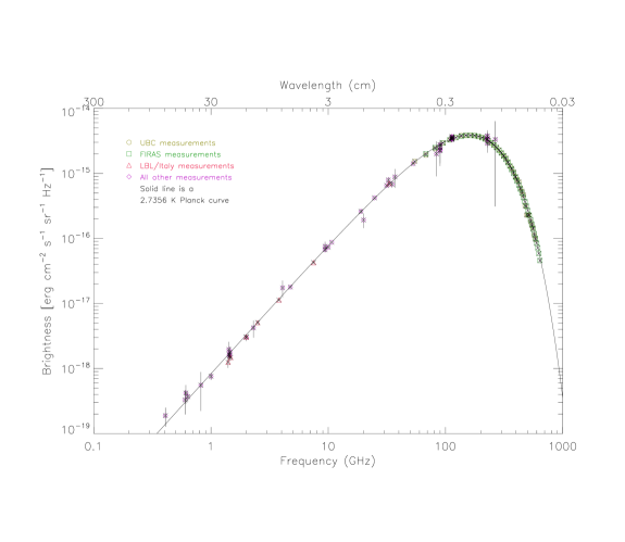
Figure 1: Brightness as a function of frequency of the CMB

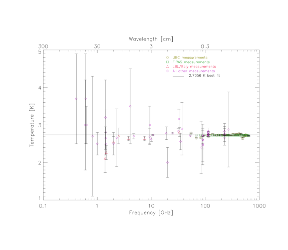
Figure 2: Thermodynamic temperature as a function of frequency of the CMB

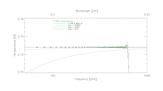
Figure 3: Thermodynamic temperature as a function of frequency of the CMB monopole. This is a close-up of Fig. 1 showing the FIRAS measurements.

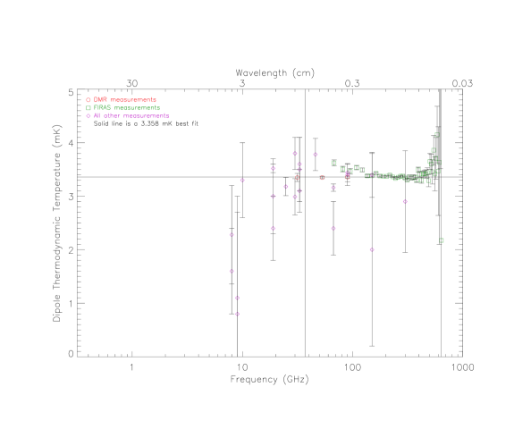
Figure 4: CMB dipole thermodynamic temperature as a function of frequency.

Figure 5: Antenna temperature for the CMB dipole with distortions versus frequency.

Figure 6: CMB dipole thermodynamic temperature as a function of frequency. This is a close-up of Fig. 5 Note the position and small errors of the COBE/DMR measurements (circles) compared to COBE/FIRAS (squares) and other measurements (diamonds).

We increased the error estimates of a few of the FIRAS and UBC points at high frequencies to account for possible systematic errors, specifically galactic dust emission removal. It is these expanded error estimates that are given in Tables The Cosmic Microwave Background Spectrum: an Analysis of Observations and 7 UBC COBRA Rocket Data; Gush et al. (1990).

4 Method

We fitted the data through finding the minimum $\chi^{2}$. Much of the data were reported as individual observations with a combined statistical and systematic error. These could in general be treated as independent, uncorrelated data points. However, much of the data including some of the most significant came from multiple observations (e.g. FIRAS, UBC, LBL) which share common systematics and calibration errors. We accounted for this via using a covariance matrix approach in calculation of $\chi^{2}$.

$$\chi^{2}\equiv(\vec{s}-\vec{t})^{T}{\bf M}^{-1}(\vec{s}-\vec{t}).$$ (25)

Here ${\bf M}$ is the covariance matrix of the data, $\vec{s}$ the signal and $\vec{t}$ the mathematical incarnation of our assumtion.

$${\bf M}\equiv[{\rm Random\;errors}]+[{\rm Correlated\;errors}]+[{\rm Theoretical\;errors}]$$ (26)

Fitting to a theory that is linear in the parameters is a simple and well developed procedure in linear algebra. For those cases where it was appropriate, we made linearized fits. When it was not appropriate we did a full non-linear fitting. We ran both approaches on a number of cases for comparison of results.

For the non-linear fitting we found that the Levenberg-Marquardt method worked well. We utilized the Levenberg-Marquardt method to iterate to the optimal $\chi^{2}$. It combines the Steepest Descent and Grid Search methods into an algorithm with a fast convergence.

Figure 3 and 4 show where the current measurements lie and where the distortions might be significant. As can be seen in the figures, the dipole might play a bigger role in determining the parameters of the distortions if more measurements were available in the region below 10 GHz.

4.1 Results

Table 1: Nonlinear fit of $T_{\rm 0}$, ${Y_{\rm ff}}$, $\mu_{\rm 0}$, $y$ and $\beta$. $\chi^{2}=259$ with 201 degrees of freedom.

$T_{0}$	=	$2.7356$	$\pm$	$0.0037$ K	(95% CL)
${Y_{\rm ff}}$	=	$-1.1\times 10^{-5}$	$\pm$	$2.3\times 10^{-5}$	(95% CL)
$\mu_{0}$	=	$-3.1\times 10^{-5}$	$\pm$	$1.2\times 10^{-4}$	(95% CL)
$y$	=	$1.6\times 10^{-6}$	$\pm$	$9.6\times 10^{-6}$	(95% CL)
$\beta$	=	$1.2293\times 10^{-3}$	$\pm$	$4.9\times 10^{-6}$	(95% CL)

Correlation matrix = $\begin{array}[]{c}\\ T_{0}\\ {Y_{\rm ff}}\\ \mu_{0}\\ y\\ \beta\end{array}\begin{array}[]{c}\\ \left[\begin{array}[]{c}\\ \\ \\ \\ \\ \end{array}\right.\end{array}\begin{array}[]{rrrrr}T_{0}&{Y_{\rm ff}}&\mu_{0}&y&\beta\\ 1.00&0.01&0.05&0.09&0.27\\ 0.01&1.00&-0.27&-0.18&0.01\\ 0.05&-0.27&1.00&0.82&-0.01\\ 0.09&-0.18&0.82&1.00&0.00\\ 0.27&0.01&-0.01&0.00&1.00\\ \end{array}\begin{array}[]{c}\\ \left.\begin{array}[]{c}\\ \\ \\ \\ \\ \end{array}\right]\end{array}$

The results of this work are new limits on the following cosmological parameters:
$T_{0}$ – the thermodynamic temperature of the background radiation
$\beta$ – the quotient of the speed of our solar system to the speed of light, $c$
${Y_{\rm ff}}$ – a measure of the effects of Bremsstrahlung, unitless; a.k.a. ${J_{\rm ff}}$
y – a measure of the effects of Compton scattering, unitless
$\mu_{0}$ – describes the Bose-Einstein distortion, unitless.
The latter three parameters are explained in section 2.1. The dipole appears because the solar system moves relative to the CMB.

The most complete fit is a nonlinear simultaneous fit of $T_{0}$, ${Y_{\rm ff}}$, $\mu_{0}$, $y$ and $\beta$, as shown in Table 1, making use of all data published for the CMB monopole and dipole. The data are dominated by the COBE FIRAS [Fixsen et al. (1996)] and the COBE DMR [Lineweaver et al. (1996)] measurements for the monopole and the dipole respectively.

Table 2 contains the best-fitted values of $T_{0}$, ${Y_{\rm ff}}$ and $\mu_{0}$. That fitting was done using both monopole and dipole data with linearized theory (see section 3 below). Table 1 includes $y$ and $\beta$, as well as the parameters in Table 2. All measurements of the CMB monopole are plotted in Figure 1 – background flux versus frequency, Figure 2 – temperature versus frequency and Figure 3 – a close-up of the most interesting part of Figure 2. The dipole is plotted in Figure 4 – dipole temperature versus frequency, Figure 6 – a close-up of Figure 4 and Figure 5 – dipole antenna temperature versus frequency.

Table 2: Linear fit with $T_{0}$, ${Y_{\rm ff}}$, $\mu_{0}$ and $y$

$T_{0}$	=	$2.7356$	$\pm$	$0.0038$ K	(95% CL)
${Y_{\rm ff}}$	=	$-1.1\times 10^{-6}$	$\pm$	$2.3\times 10^{-5}$	(95% CL)
$\mu_{0}$	=	$-3.0\times 10^{-5}$	$\pm$	$1.2\times 10^{-4}$	(95% CL)
$y$	=	$1.6\times 10^{-6}$	$\pm$	$9.6\times 10^{-6}$	(95% CL)

Correlation matrix = $\begin{array}[]{c}\\ T_{0}\\ {Y_{\rm ff}}\\ \mu_{0}\\ y\end{array}\begin{array}[]{c}\\ \left[\begin{array}[]{c}\\ \\ \\ \\ \end{array}\right.\end{array}\begin{array}[]{rrrr}T_{0}&{Y_{\rm ff}}&\mu_{0}&y\\ 1.00&0.03&-0.02&0.00\\ 0.03&1.00&-0.28&-0.18\\ -0.02&-0.28&1.00&0.82\\ 0.00&-0.18&0.82&1.00\\ \end{array}\begin{array}[]{c}\\ \left.\begin{array}[]{c}\\ \\ \\ \\ \end{array}\right]\end{array}$

Table 3: Non-linear fit with $T_{0}$, ${Y_{\rm ff}}$, $\mu_{0}$ and $y$ to CMB spectrum monopole. No dipole data included.

$T_{0}$	=	$2.7377$	$\pm$	$0.0038$ K	(95% CL)
${Y_{\rm ff}}$	=	$-1.1\times 10^{-5}$	$\pm$	$2.3\times 10^{-5}$	(95% CL)
$\mu_{0}$	=	$-3.0\times 10^{-5}$	$\pm$	$1.2\times 10^{-4}$	(95% CL)
$y$	=	$1.6\times 10^{-6}$	$\pm$	$9.6\times 10^{-6}$	(95% CL)

Correlation matrix = $\begin{array}[]{c}\\ T_{0}\\ {Y_{\rm ff}}\\ \mu_{0}\\ y\end{array}\begin{array}[]{c}\\ \left[\begin{array}[]{c}\\ \\ \\ \\ \end{array}\right.\end{array}\begin{array}[]{rrrr}T_{0}&{Y_{\rm ff}}&\mu_{0}&y\\ 1.00&0.01&0.06&0.09\\ 0.01&1.00&-0.27&-0.18\\ 0.06&-0.27&1.00&0.82\\ 0.09&-0.18&0.82&1.00\\ \end{array}\begin{array}[]{c}\\ \left.\begin{array}[]{c}\\ \\ \\ \\ \end{array}\right]\end{array}$

5 Analysis of the Cosmic Microwave Background Spectrum

A novelty of this analysis has been to use the dependence on frequency for the distortions of the dipole in the fits. Using the dipole data in the fit only marginally improved the fit, however. This is due to the particular frequencies of the dipole measurements. Figure 4 shows the current measurements versus frequency and where the distortions are significant. As can be seen in Figure 4, the dipole may play a bigger role in determining the parameters of the distortions when more measurements, with much greater precision or in the region below 10 GHz, become available. Using the dipole does provide an independent check of the spectrum data.

Figure 7: Upper limits (95% CL) on fractional energy ($\Delta E/E_{CBR}$) releases. $\Omega_{b}$ is the baryon number density and $h$ is the hubble expansion rate per 100 km s^-1 Mpc^-1 .

Figure 7 shows upper limits (95% CL) on fractional energy ($\Delta E/E_{CBR}$) releases as set by lack of CMB spectral distortions resulting from processes at different epochs. These can be translated into constraints on the mass, lifetime and photon branching ratio of unstable relic particles, with some additional dependence on cosmological parameters such as $\Omega_{\rm b}$, the baryon number density [Hu & Silk (1993), Wright et al. (1994)].

5.1 Some Interpretation of Limits

The greatest significance of the non-detection of distortions in the CMB spectrum is the support it gives to the Hot Big Bang model of cosmology. A blackbody spectrum is the natural result of a system in thermal equilibrium; conversely, it is very difficult to superpose a set of non-thermal spectra to mimic a blackbody to such tight tolerance over so broad a frequency range. Steady-state models generally create a microwave background by absorption and subsequent re-emission of starlight by dust. The re-emitted photons are then redshifted by the expansion of the universe, so that we observe a superposition of “shells” radiating at different epochs. If the dust opacity were independent of frequency, the microwave background would be a superposition of thermal spectra redshifted to different temperatures, equivalent to a Compton $y$ distortion. The dust opacity can be tailored to bring the superposition closer to a blackbody, but the required (very high) opacities at millimeter wavelengths conflict with direct observations of high-redshift galaxies at these wavelengths [Peebles (1993) p203-6].

The same basic arguments rule out “plasma universes” models.

5.1.1 Stucture Formation by Explosions

The lack of spectral distortions has implications for structure formation. Explosive models of structure formation provide a simple way to sweep (baryonic) matter out of the observed voids. The resulting shocks, however, heat the baryons and distort the CMB spectrum. Upper limits on a Compton $y$ distortion limit the maximum size of explosive voids to $R_{\rm void}<2$ Mpc, much smaller than the observed voids [Levin et al. (1992)].

5.1.2 Temperature of the Ionization of the Intergalactic Medium

The good agreement with a blackbody spectrum also tells us something about the intergalactic medium (IGM). A hot ($T_{\rm e}>10^{6}$ K) IGM would provide the high ionization inferred by the lack of a Gunn-Peterson absorption trough in the spectra of high-redshift quasars. Thermal bremsstrahlung from the hot gas would provide a natural source for the observed diffuse X-ray background. However, a column density large enough to explain the X-ray background would create an observable Compton $y$ distortion in the CMB spectrum. Upper limits on the $y$ parameter limit the filling factor of hot gas to less than $10^{-4}$: the diffuse IGM is not very hot, and the X-ray background must come from discrete (collapsed) sources [Wright et al. (1994)].

5.1.3 Limits on Particle Decay

Exotic particle decay provides another source for non-zero chemical potential. Particle physics provides a number of dark matter candidates, including massive neutrinos, photinos, axions, or other weakly interacting massive particles (WIMPs). In most of these models, the current dark matter consists of the lightest stable member of a family of related particles, produced by pair creation in the early universe. Decay of the heavier, unstable members to a photon or charged particle branch will distort the CMB spectrum provided the particle lifetime is greater than a year. Rare decays of quasi-stable particles (e.g., a small branching ratio for massive neutrino decay $\nu_{\rm heavy}\rightarrow\nu_{\rm light}+\gamma$) provide a continuous energy input, also distorting the CMB spectrum. The size and wavelength of the CMB distortion are dependent upon the decay mass difference, branching ratio, and lifetime. Stringent limits on the energy released by exotic particle decay provides an important input to high-energy theories including supersymmetry and neutrino physics [Ellis et al. (1992)].

5.1.4 Limits on Antimatter-matter mixing

In baryon symmetric cosmologies matter-antimatter annihilations give rise to excessive distortions of the CMB spectrum [Jones & Steigman (1978)].

5.1.5 Limits on Primordial Black Hole Evaporation

Only a very small fraction, $f=M_{planck}/M$, of matter can have formed black holes in the mass range $10^{11}\leq M\leq 10^{13}$ gm otherwise their evaporation in the epoch preceding recombination would have resulted in excessive distortions. For smaller blackholes the limit is much weaker, since for $M<10^{11}$ gm, evaporation would have taken place during the epoch when the photon spectrum would be completely thermalized. The constraints follow from the condition that no more than all the entropy in the universe can come from blackhole evaporation so that $f<10^{9}M_{planck}/M$.

5.1.6 Limits on Superconducting Cosmic Strings

If they are to play an important role in large-scale structure formation, superconducting cosmic strings would be significant energy sources, keeping the Universe ionized well past standard recombination. As a result, the energy input distorts the spectrum of the CMB by the Sunyaev-Zel’dovich effect. The Compton-$y$ parameter attains a maximum value in the range of $(1-5)\times 10^{-3}$ [Ostriker & Thompson (1987)]. This is well above the observed value.

5.1.7 Limits on Varying Fundamental Constants

Noerdlinger [1973] pointed out that the intensity of the Rayleigh-Jeans portion of the CMB spectrum gives the present values of $kT$, independently of the value of the Planck constant, $h$, while the wavelength at which the spectrum peaks gives $kT$ in combination with $h$. That the two temperatures agree within errors imply that the variation of $h$ must not have exceeded a few per cent since recombination ($z\sim 1000$). Likewise a wide variety of $G$-varying cosmologies predict that the CMB spectrum will follow the standard Planckian formula multiplied by an epoch-dependent factor, which, in turn, is related to $G(t)$ [Narlikar & Rana (1980)]. The agreement between the brightness temperature in the Rayleigh-Jeans region and the temperature determined by the peak location constrain the possible variation in the gravitational constant $G$. Likewise one can obtain limits on the variation in the cosmological constant (energy density of the vacuum) [Pollock (1973)]. The shape of the spectrum also constrains the number of large spatial dimension (taking into account the possibility of fractal dimensions) to very nearly three ($\pm 0.02$).

5.1.8 Limits on Tachyon Coupling Constant

The existence of particles with space-like four-momenta (“tachyons”) would make it kinematically possible for a photon to decay into a pair of tachyons. If tachyons have any electromagnetic coupling, photons should have finite lifetimes. Lorentz invariance dictates that the laboratory lifetime of a particle scales in proportion to its observed energy ($\gamma$). The temperature of the CMB does not vary by more than 1% over the range of wavelengths from 0.05 to 1 cm.

Assuming, as would be expected, that the radiation was in thermal equilibrium when last scattered at a redshift of about 1100, the absence of spectral distortions, which would result from the differential (with energy) photon decay rates acting over time, argues that the lifetime of microwave photons must be ${{}_{>}\atop{}^{\sim}}$ 40 Hubble times. (Note that the photons begin with energies a thousand times higher than they currently have and thus the effective time for decay is about 40% of the Hubble time.)

This argument [Shapiro (1991)] sets a more stringent upper limit on the coupling of tachyons to photons than has previously been reported [Baltay et al. (1970)].

5.1.9 Limits on Photon Mass/Oscillations/Paraphotons

Georgi, Ginsparg, & Glashow (1983) and Okun (1982) hypothesized the exisitence of a second species of photon whose coupling could produce photon masses and photon species oscillation. The oscillations of photon identity are entirely analogous to the much-discussed neutrino oscillations. Though the photon mass would have to be much lower than current experimental limits ($m_{\gamma}\leq 6\times 10^{-16}$ eV $c^{-2}$ at 99.7% CL), Georgi et al. showed that a photon mass at the $m_{\gamma}=5\times 10^{-18}$ eV $c^{-2}$ could produce distortions much beyond what is now allowed by the CMB spectrum observations.

The second species of photon would have a very weak interaction with matter and therefore not have been detected thus far. This new species of photon would have decoupled much earlier in the big bang and have a lower temperature than the detected CMB, since its decoupling would occur earlier. The intensity of the interacting/oscillating photon species is given by

$$I(\nu)=I_{BB}(\nu,T_{1})+[I_{BB}(\nu,T_{2})-I_{BB}(\nu,T_{1})]sin^{2}(2\phi)sin^{2}(\pi\nu_{0}/\nu)$$ (27)

where $I_{BB}$ is the standard blackbody Planckian spectrum, and $T_{1}$ and $T_{2}$ are the temperature of the two photon species, $\phi$ is the mixing phase angle, and $\nu_{0}=3\Delta m_{\gamma}^{2}c^{4}\tau/40\pi^{2}\hbar^{2}=8.2875\Delta(m_{\gamma}c^{2}/10^{-18}~{}{\rm eV})^{2}~{}{\rm GHz}$ for $\tau=1.5\times 10^{10}$ years for the age of the Universe (and thus the travel time for the photons).

This manifests itself as an oscillation with frequency of the observed CMB intensity or temperature.

This oscillation is very enhanced in the dipole amplitude and could even change the sign of the dipole as the dipole amplitude is related to the derivative of the intensity with respect to frequency and there is a one over frequency ($\nu$) in the intensity oscillations.

$$\Delta n = {\beta\over\nu}\left({x_{1}e^{x_{1}}\over(e^{x_{1}}-1)^{2}}+sin^{2}(2\phi)\left[\left({x_{2}e^{x_{2}}\over(e^{x_{2}}-1)^{2}}-{x_{1}e^{x_{1}}\over(e^{x_{1}}-1)^{2}}\right)sin^{2}({\pi\nu_{0}\over\nu})+({1\over e^{x_{2}}-1}-{1\over e^{x_{1}}-1})sin({2\pi\nu_{0}\over\nu}){\pi\nu_{0}\over\nu}\right]\right)$$ (28)

$${\Delta n\over n}\approx\beta\left({x_{1}e^{x_{1}}\over e^{x_{1}}-1}+sin^{2}(2\phi)\left[\left({x_{1}e^{x_{1}}\over e^{x_{1}}-1}-{x_{2}e^{x_{2}}\over e^{x_{2}}-1}\right)sin^{2}({\pi\nu_{0}\over\nu})-{e^{x_{1}}-e^{x_{2}}\over e^{x_{2}}-1}sin({2\pi\nu_{0}\over\nu}){\pi\nu_{0}\over\nu}\right]\right)$$ (29)

Figures 8 and 9 show the spectral monopole and dipole distortion for the effect of such an oscillation with the parameters: $sin^{2}(2\phi)=0.35$, $T_{1}=2.74$ K, $T_{2}=2$ K, and $\Delta m_{\gamma}c^{2}=1\times 10^{-18}$ eV and $\Delta m_{\gamma}c^{2}=0.25\times 10^{-18}$ eV .

Figure 8: Thermodynamic temperature as a function of frequency of the CMB for all measurements along with a plot of two photon oscillations with $\Delta m_{\gamma}^{2}=(1\times 10^{-18}{\rm eV/c^{2}})^{2}$, $\Delta m_{\gamma}^{2}=(0.25\times 10^{-18}{\rm eV/c^{2}})^{2}$, $sin^{2}(2\phi)=0.35$ and $T_{2\gamma}=2.0$ K.

Figure 9: Dipole amplitude in thermodynamic temperature as a function of frequency of the CMB for all measurements along with a plot of two photon oscillations with $\Delta m_{\gamma}^{2}=(1\times 10^{-18}{\rm eV/c^{2}})^{2}$, $\Delta m_{\gamma}^{2}=(0.25\times 10^{-18}{\rm eV/c^{2}})^{2}$, $sin^{2}(2\phi)=0.35$ and $T_{2\gamma}=2.0$ K.

Figure 10 shows a contour plot of the $\chi^{2}$ (chi-squared) in the $sin^{2}2\phi$ versus $\Delta m_{\gamma}^{2}$ plane of the two-photon oscillating model as fitted to the data. This plot has minimized $\chi^{2}$ for the other parameters: $T_{CMB}$, $\beta$, and the temperature of the second photon constrained to be between 0.9 and 2.0 K. In addition to having a very large region ruled out, there is a clear minimum in the $\chi^{2}$ at roughly $\Delta m_{\gamma}^{2}=(0.25\times 10^{-18}{\rm eV/c^{2}})^{2}$ and $sin^{2}(2\phi)=0.35$ in the all data plot. As can be seen in Figure 8 the minimum is due essentially to a limited set of the low frequency temperature data which are slightly lower than the average. Such a low photon mass difference produces a lowering of the predicted temperature at these lower frequencies. Other than the minimum in $\chi^{2}$, there is little evidence here by the data tracing out the expected form for photon oscillations. Thus while suggestive, we regard the results thus far as an upper limit set at a slightly higher $\chi^{2}$ than normal and await future measurements.

Note that going from $\Delta m_{\gamma}^{2}=(0.25\times 10^{-18}{\rm eV/c^{2}})^{2}$ to $\Delta m_{\gamma}^{2}=(1\times 10^{-18}{\rm eV/c^{2}})^{2}$ moves the frequency of the oscillations/effect upwards by a factor or 16 and is easily ruled out by both the temperature and dipole amplitude data. Also know the potential power of low frequency dipole amplitude measurements for discriminating photon oscillations.

Figure 10: Contour plot of $\chi^{2}$ on a plane of $sin^{2}(2\phi)$ versus $\Delta m_{\gamma}^{2}$ which is marginalized over the other parameters. The $\chi^{2}$ is for all measurements – temperature and dipole anisotropy amplitude.

5.2 Lower Limits on the Distortions

Observations show that the universe is ionized [Haiman & Loeb (1997)]. The ionized intergalactic medium creates bremsstrahlung and sets a lower limit on the free-free distortion to ${Y_{\rm ff}}\sim 2\times 10^{-6}$. This results in an added temperature of $\Delta T_{\rm ff}>0.15$ mK at 2 GHz (as low as one might reasonably go in frequency, due to synchrotron emision from the galaxy). This result only takes into account the observed baryons. The actual distortion is bigger, because this limit did not include bremsstrahlung that may have occured at earlier epochs.

A lower limit on the Compton distortion is obtained from measurements of the Sunyaev-Zeldovich effect [Sunyaev & Zeldovich (1970)]. The SZ effect is due to hot ionized plasma component of galactic clusters. This plasma creates a $y$ for paths that go through the cores of galactic clusters. Ionized gases in these potential wells Compton-scatter the passing photons. Integrating over the full sky, $y$ is of the order of $10^{-6}$ [Colafrancesco et al. (1997)].

Density fluctuations in the early universe oscillate as acoustic waves and are damped by photon diffusion [Silk (1968)]. The energy dissipated in this manner is added to the radiation field and gives rise to a non-zero chemical potential. Depending on the nature of the density fluctuations, $\mu$ will lie between $2\times 10^{-8}$ and a few times $10^{-5}$ [Daly (1991), Hu et al. (1994)].

6 Future Experiments

Even though no significant distortions to the CMB spectrum have been detected and since many of the distortions predicted and required by known effects are not much below current limits, it is worth considering if future experiments will detect them. There are two hinderances: (1) the current limits, especially those set by COBE FIRAS, are quite good and (2) there is currently a limited effort in spectrum observations in part due to (1) and to the high interest in CMB anisotropy and due to a lack of appreciation that the spectral distortions are there to detect.

Since the distortions are frequency dependent an absence of them at millimeter and sub-mm wavelengths does not imply correspondingly small distortions at centimeter wavelengths. A better understanding of Galactic emissions, especially at longer wavelengths, would help produce tighter limits on the distortion parameters. It would be difficult to improve on the COBE measurements without getting above the atmosphere. There are, nevertheless, proposals for new experiments that will measure the CMB.

ARCADE (Absolute Radiometer for Cosmology, Astrophysics, and Diffuse Emission) is a balloon-borne instrument designed to make measurements in the middle of the spectrum. The first flight will have two channels at 10 and 30 GHz. Later incarnations will measure the spectrum at 2, 4, 6, 10, 30 and 90 GHz.

The anticipated measurement sensitivity is 1 mK from a balloon, limited by the ability to estimate/measure emissions from the atmosphere, balloon, flight train, and Earth. ARCADE is also a hardware development project for the proposed eventual space mission, DIMES.

The Diffuse Microwave Emission Survey (DIMES) has been selected for a mission concept study for NASA’s New Mission Concepts for Astrophysics program [Kogut (1996), http://ceylon.gsfc.nasa.gov/DIMES/index.html]. DIMES will measure the frequency spectrum of the cosmic microwave background and diffuse Galactic foregrounds at centimeter wavelengths to 0.1% precision (0.1 mK). Note that this should detect the free-free distortion, the lower limit of which was mentioned in section 5.2.

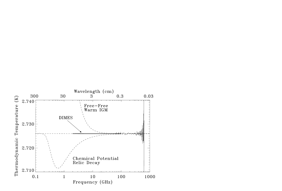
Figure 11: Current 95% confidence upper limits to distorted CMB spectra appear as dashed lines. The FIRAS data and DIMES 0.1 mK error box are also shown; error bars from existing cm-wavelength measurements are larger than the figure height.

The FIRAS measurement at sub-mm wavelengths shows no evidence for Compton heating from a hot IGM (Inter-Galactic Medium). Since the Compton parameter $y\propto n_{e}T_{e}$, the IGM at high redshift must not be very hot ($T_{e}\sim 10^{5}$ K) or reionization must occur relatively recently ($z_{\rm ion}<10$). DIMES will provide a definitive test of these alternatives. Since the free-free distortion $Y_{\rm ff}\propto n_{e}^{2}/\sqrt{T_{e}}$, lowering the electron temperature increases the spectral distortion [Bartlett & Stebbins (1991)]. Figure 11 shows the limit to $z_{\rm ion}$ that could be established from the combined DIMES and FIRAS spectra, as a function of the DIMES sensitivity. A spectral measurement at centimeter wavelengths with 0.1 mK precision can detect the free-free signature from the ionized IGM, allowing direct detection of the onset of hydrogen burning.

ESA’s Planck Surveyor mission to map CMB anisotropy is capable of measuring the CMB dipole with sufficient accuracy to provide limits at about the current level provided by COBE FIRAS + DMR in a very independent manner. This would provide a significant cross-check of these results and perhaps a small improvement in net results. It will require dedicated missions such as DIMES to make a really significant improvement.

7 Summary

None of the distortions, $y,{Y_{\rm ff}}$ or $\mu$, are larger than the current errors in measurement for the monopole and dipole CMB spectra. The monopole CMB spectrum is very close to a blackbody spectrum. This is strong evidence of the validity of the hot Big Bang model [Smoot (1996)] because there are roughly $10^{9}$ photons to each baryon in the universe, and it would be extremely difficult to produce the CMB in astrophysical processes such as the absorption and re-emission of starlight by cold dust, or the absorption or emission by plasmas, and still produce such a precise black body spectrum.

The dipole data did not significantly improve on the errors, but were consistent with and an independent check of the monopole data. Future measurements of the dipole could potentially contribute to tightening the limits or detecting distortions. The Planck Surveyor measurements of the dipole could, in principle, determine the distortions to approximately the same precision as the monopole measurements do now. Very substantial progress that would surely detect the predicted distortions and provide us with new information on the thermal history of the Universe will require a significant dedicated mission.

8 Acknowledgments

We thank Dr. Alan Kogut for providing us with information on DIMES. We also thank Dr. S.Y. Frank Chu (LBNL), for his insight into numerical programming.

This work supported in part by the DOE contract No. DE-AC03-76SF00098 through the Lawrence Berkeley National Laboratory.

Dipole References

Bennett, C.L., et al. 1994, Astrophysical Journal, 436, 423
Bennett, C.L., et al. 1996, Astrophysical Journal, 464, L1-4
Boughn, S.P. et al. 1971, Astrophysical Journal, 165, 439
Boughn, S.P. et al. 1981, Astrophysical Journal, 243, L113
Cheng, E.S. et al. 1979, Astrophysical Journal, 232, L139
Cheng, E.S. 1983 Ph.D. thesis, Princeton Univ.
Conklin, E.K. 1969, Nature, 222, 971
Conklin, E.K. 1972, IAU Symposium 44, ed. D.S. Evans (Dordrecht: Reidel), 518
Corey, B.E. 1978, Ph.D. thesis Princeton U.
Corey, B.E. & Wilkinson D. T., 1976, Bull. Amer. Astron. Soc, 8, 351
Cottingham, D.A. 1987, Ph.D. thesis, Princeton Univ.
Fabbri, R., et al. 1980, Phys. Rev. Let., 44, 1563, erratum 1980, Phys. Rev. Let., 45, 401
Fixsen, D.J., Cheng, E.S. & Wilkinson, D.T. 1983, Phys. Rev. Let., 50, 620
Fixsen, D.J., et al. 1994, Astrophysical Journal, 420, 445
Fixsen, D.J., et al. 1996, Astrophysical Journal, 486, 623
Ganga, K., Cheng, E., Meyer, S., Page, L. 1993, Astrophysical Journal, 410, L57
Gorenstein, M.V. 1978, Ph.D. thesis, U.C. Berkeley
Halpern, M., et al. 1988 Astrophysical Journal, 332, 596
Henry, P.S. 1971, Nature, 231, 516
Kogut, A., et al. 1993, Astrophysical Journal, 419, 1
Lineweaver, C.H., et al. 1995, Astrophysical Letters and Comm., 32, 173-181
Lineweaver, C.H., et al. 1996, Astrophysical Journal, 470, 38
Lubin, P.M., Epstein, G.L., Smoot, G.F. 1983, Phys. Rev. Let., 50, 616
Lubin, P.M. et al. 1985, Astrophysical Journal, 298, L1
Meyer, S.S., et al. 1991, Astrophysical Journal, 371, L7
Muehler, D. 1976, in Infrared and Submillimeter Ast., ed G.Fazio, D.Reidel, Dordrecht, 63
Partridge, R.B. & Wilkinson, D. T., 1967, Phys. Rev. Let.18, 557
Penzias, A.A. & Wilson, R. W. 1965, Astrophysical Journal, 142, 419
Smoot, G.F., Gorenstein, M. V. & Muller, R. A. 1977, Phys. Rev. Let., 39, 898
Smoot, G.F. & Lubin, P. 1979, Astrophysical Journal, 234, L83
Smoot, G.F., et al. 1991, Astrophysical Journal, 371, L1
Smoot, G.F., et al. 1992, Astrophysical Journal, 396, L1
Strukov, I.A., Skulachev, D.P. 1984, Sov. Ast. Lett. 10, 3
Strukov, I.A., Skulachev, D.P., Boyarskii, M.N., Tkachev, A.N. 1987, Sov. Ast. Lett. 13, 2
Wilkinson, D.T. & Partridge, R.B. 1969, Partridge quoted in American Scientist, 57, 37

Table 4: All dipole data used in the fits. Coordinates are galactic.

	Amplitude	Longitude	Latitude	Freq
	[mK]	l [deg]	b [deg]	[GHz]
Penzias & Wilson (1965)	$<$270			4
Partridge & Wilkinson (1967)	0.8 $\pm$ 2.2			9
Wilkinson & Partridge (1969)	1.1 $\pm$ 1.6			9
Conklin (1969)	1.6 $\pm$ 0.8	96 $\pm$ 30	85 $\pm$ 30	8
Boughn et al. (1971)	7.6 $\pm$ 11.6			37
Henry (1971)	3.3 $\pm$ 0.7	270 $\pm$ 30	24 $\pm$ 25	10
Conklin (1972)	$>$2.28 $\pm$ 0.92	195 $\pm$ 30	66 $\pm$ 10	8
Corey & Wilkinson (1976)	2.4 $\pm$ 0.6	306 $\pm$ 28	38 $\pm$ 20	19
Muehler (1976)	2.0 $\pm$ 1.8	207	-11	150
Smoot et al. (1977)	3.5 $\pm$ 0.6	248 $\pm$ 15	56 $\pm$ 10	33
Corey (1978)	3.0 $\pm$ 0.7	288 $\pm$ 26	43 $\pm$ 19	19
Gorenstein (1978)	3.60 $\pm$ 0.5	229 $\pm$ 11	67 $\pm$ 8	33
Cheng et al. (1979)	2.99 $\pm$ 0.34	287 $\pm$ 9	61 $\pm$ 6	30
Smoot & Lubin (1979)	3.1 $\pm$ 0.4	250.6 $\pm$ 9	63.2 $\pm$ 6	33
Fabbri et al. (1980)	2.9 $\pm$ 0.95	256.7 $\pm$ 13.8	57.4 $\pm$ 7.7	300
Boughn et al. (1981)	3.78 $\pm$ 0.30	275.4 $\pm$ 3.9	46.8 $\pm$ 4.5	46
Cheng (1983)	3.8 $\pm$ 0.3			30
Fixsen et al. (1983)	3.18 $\pm$ 0.17	265.7 $\pm$ 3.0	47.3 $\pm$ 1.5	25
Lubin (1983)	3.4 $\pm$ 0.2			90
Strukov et al. (1984)	2.4 $\pm$ 0.5			67
Lubin et al. (1985)	3.44 $\pm$ 0.17	264.3 $\pm$ 1.9	49.2 $\pm$ 1.3	90
Cottingham (1987)	3.52 $\pm$ 0.08	272.2 $\pm$ 2.3	49.9 $\pm$ 1.5	19
Strukov et al. (1987)	3.16 $\pm$ 0.07	266.4 $\pm$ 2.3	48.5 $\pm$ 1.6	67
Halpern et al. (1988)	3.4 $\pm$ 0.42	289.5 $\pm$ 4.1	38.4 $\pm$ 4.8	150
Meyer et al. (1991)	$\pm$	249.9 $\pm$ 4.5	47.7 $\pm$ 3.0	170
Smoot et al. (1991)	3.3 $\pm$ 0.1	265 $\pm$ 1	48 $\pm$ 1	53
Smoot et al. (1992)	3.36 $\pm$ 0.1	264.7 $\pm$ 0.8	48.2 $\pm$ 0.5	53
Ganga et al. (1993)	$\pm$	267.0 $\pm$ 1.0	49.0 $\pm$ 0.7	170
Kogut et al. (1993)	3.365 $\pm$ 0.027	264.4 $\pm$ 0.3	48.4 $\pm$ 0.5	53
Fixsen et al. (1994)	3.347 $\pm$ 0.008	265.6 $\pm$ 0.75	48.3 $\pm$ 0.5	300
Bennett et al. (1994)	3.363 $\pm$ 0.024	264.4 $\pm$ 0.2	48.1 $\pm$ 0.4	53
Bennett et al. (1996)	3.353 $\pm$ 0.024	264.26$\pm$ 0.33	48.22 $\pm$ 0.13	53
Fixsen et al. (1996)	3.372 $\pm$ 0.005	264.14$\pm$ 0.17	48.26 $\pm$ 0.16	300
Lineweaver et al. (1996)	3.358 $\pm$ 0.023	264.31$\pm$ 0.17	48.05 $\pm$ 0.10	53

Table 5: Measurements of $T_{\rm CMB}$

Frequency	Wavelength	Temperature	Type	Reference
(GHz)	(cm)	(K)
0.408	73.5	$3.7\pm 1.2$	Ground (LN)	Howell & Shakeshaft 1967, Nature, 216, 753.
0.6	50	$3.0\pm 1.2$	Ground (Term)	Sironi et al. 1990, Ap.J., 357, 301.
0.610	49.1	$3.7\pm 1.2$	Ground (LN)	Howell & Shakeshaft 1967, Nature, 216, 7
0.635	47.2	$3.0\pm 0.5$	Ground (LN)	Stankevich et al 1970, Australian J. Phys, 23, 529
0.820	36.6	$2.7\pm 1.6$	Ground (Term)	Sironi et al. 1991, Ap.J., 378, 550.
1	30	$2.5\pm 0.3$	Ground (LN)	Pelyushenko & Stankevich 1969, Sov. Astron., 13, 223.
1.4	21.3	$2.11\pm 0.38$	Ground (CLC)	Levin et al. 1988, Ap.J., 334,14
1.42	21.2	$3.2\pm 1.0$	Ground (Term)	Penzias and Wilson 1967, AJ, 72, 315
1.43	21	$2.65^{+0.33}_{-0.30}$	Ground (LN)	Staggs et al. 1996, ApJ, 458, 407
1.44	20.9	$2.5\pm 0.3$	Ground (LN)	Pelyushenko & Stankevich 1969, Sov. Astron., 13, 223.
1.45	20.7	$2.8\pm 0.6$	Ground (Term)	Howell & Shakeshaft 1966, Nature, 210, 1318.
1.47	20.4	$2.27\pm 0.19$	Ground (CLC)	Bensadoun et al. 1993, Ann. NY Acad. Sci, 668, p792-4
2	15	$2.5\pm 0.3$	Ground (LN)	Pelyushenko & Stankevich 1969, Sov. Astron., 13, 223.
2	15	$2.55\pm 0.14$	Ground (CLC)	Bersanelli et al., 1994, Ap.J., 424, 517
2.3	13.1	$2.66\pm 0.77$	Ground (Term)	Otoshi & Stelzreid 1975, IEEE Trans on Inst & Meas, 24, 174.
2.5	12	$2.71\pm 0.21$	Ground (CLC)	Sironi et al. 1991, Ap. J., 378, 550.
3.8	7.9	$2.64\pm 0.06$	Ground (CLC)	De Amici et al. 1991, Ap.J., 381, 341.
4.08	7.35	$3.5\pm 1.0$	Ground (Term)	Penzias & Wilson 1965, Ap.J., 142, 419.
4.75	6.3	$2.70\pm 0.07$	Ground (CLC)	Mandolesi et al. 1986, Ap.J., 310, 561.
7.5	4.0	$2.60\pm 0.07$	Ground (CLC)	Kogut et al. 1988, Ap.J., 355, 102
7.5	4.0	$2.64\pm 0.06$	Ground (CLC)	Levin et al. 1992, Ap.J., 396, 3
9.4	3.2	$3.0\pm 0.5$	Ground (Term)	Roll & Wilkinson 1966, Phys. Rev. Lett., 16, 405.
9.4	3.2	$2.69^{+0.16}_{-0.21}$	Ground (CLC)	Stokes et al. 1967, Phys. Rev. Lett., 19, 1199.
10	3.0	$2.62\pm 0.06$	Ground (CLC)	Kogut et al. 1990, Ap.J., 355, 102.
10.7	2.8	$2.730\pm 0.014$	Balloon (LHe)	Staggs et al. 1996, Ap.J., 473, L1
19.0	1.58	$2.78^{+0.12}_{-0.17}$	Ground (CLC)	Stokes et al. 1967, Phys. Rev. Lett., 19, 1199.
20	1.5	$2.0\pm 0.4$	Ground (CLC)	Welch et al. 1967, Phys. Rev. Lett, 18, 1068.
24.8	1.2	$2.783\pm 0.025$	Balloon	Johnson & Wilkinson 1987, Ap.J. Lett, 313, L1.

Table 5: Measurements of $T_{\rm CMB}$ continued

Frequency	Wavelength	Temperature	Type	Reference
(GHz)	(cm)	(K)
31.5	0.95	$2.83\pm 0.07$	COBE/DMR	Kogut et al. 1996, Ap.J, 470, 653
32.5	0.924	$3.16\pm 0.26$	Ground (CLC)	Ewing et al. 1967, Phys. Rev. Lett, 19, 1251.
33.0	0.909	$2.81\pm 0.12$	Ground (CLC)	De Amici et al. 1985, Ap.J., 298, 710.
35.0	0.856	$2.56^{+0.17}_{-0.22}$	Ground (CLC)	Wilkinson 1967, Phys. Rev. Lett., 19, 1195.
37	0.82	$2.9\pm 0.7$	Ground (LN)	Puzanov et al. 1968, Sov. Astr., 11, 905.
53	0.57	$2.71\pm 0.03$	COBE/DMR	Kogut et al. 1996, Ap.J, 470, 653
83.8	0.358	$2.4\pm 0.7$	Ground (LN)	Kislyakov et al. 1971, Sov. Ast., 15, 29.
90	0.33	$2.46^{+0.40}_{-0.44}$	Ground (CLC)	Boynton et al. 1968, Phys. Rev. Lett., 21, 462.
90	0.33	$2.61\pm 0.25$	Ground (CLC)	Millea et al. 1971, Phys. Rev. Lett., 26, 919.
90	0.33	$2.48\pm 0.54$	Plane (Term)	Boynton & Stokes 1974, Nature, 247, 528.
90	0.33	$2.60\pm 0.09$	Ground (CLC)	Bersanelli et al. 1989, Ap.J., 339, 632.
90	0.33	$2.712\pm 0.020$	Ground (CLC)	Schuster et al. UC Berkeley PhD Thesis
90	0.33	$2.72\pm 0.04$	COBE/DMR	Kogut et al. 1996, Ap.J, 470, 653
90.3	0.332	$<2.97$	Balloon	Bernstein et al. 1990, Ap.J., 362, 107.
113.6	0.264	$2.70\pm 0.04$	CN (z Per)	Meyer & Jura 1985, Ap.J., 297, 119.
113.6	0.264	$2.74\pm 0.05$	CN (z Oph)	Crane et al. 1986, Ap.J., 309, 12.
113.6	0.264	$2.76\pm 0.07$	CN (HD 21483)	Meyer et al. 1989, Ap.J. Lett, 343, L1.
113.6	0.264	$2.796^{+0.014}_{-0.039}$	CN (z Oph)	Crane et al. 1989, Ap.J., 346, 136.
113.6	0.264	$2.75\pm 0.04$	CN (z Per)	Kaiser & Wright 1990, Ap.J. Lett, 356, L1.
113.6	0.264	$2.834\pm 0.085$	CN (HD 154368)	Palazzi et al. 1990, Ap.J., 357, 14.
113.6	0.264	$2.807\pm 0.025$	CN (16 stars)	Palazzi et al. 1992, Ap.J., 398, 53.
113.6	0.264	$2.279^{+0.023}_{-0.031}$	CN (5 stars)	Roth et al. 1993, Ap.J., 413, L67.
154.8	0.194	$<3.02$	Balloon	Bernstein et al. 1990, Ap.J., 362, 107.
195.0	0.154	$<2.91$	Balloon	Bernstein et al. 1990, Ap.J., 362, 107.
227.3	0.132	$2.656\pm 0.057$	CN (5 stars)	Roth et al. 1993, Ap.J., 413, L67.
227.3	0.132	$2.76\pm 0.20$	CN (z Per)	Meyer & Jura 1985, Ap.J., 297, 119.
227.3	0.132	$2.75^{+0.24}_{-0.29}$	CN (z Oph)	Crane et al. 1986, Ap.J., 309, 822.
227.3	0.132	$2.83\pm 0.09$	CN (HD 21483)	Meyer et al. 1989, Ap.J. Lett, 343, L1.
227.3	0.132	$2.832\pm 0.072$	CN (HD 154368)	Palazzi et al. 1990, Ap.J., 357, 14.
266.4	0.113	$<2.88$	Balloon	Bernstein et al. 1990, Ap.J., 362, 107.
See Tab. The Cosmic Microwave Background Spectrum: an Analysis of Observations	See Tab. The Cosmic Microwave Background Spectrum: an Analysis of Observations	$2.728\pm 0.002$	COBE/FIRAS	Fixsen et al. 1996, Ap.J., 486, 623.
300	0.1	$2.736\pm 0.017$	Rocket	Gush et al. 1990, PRL, 65, 537., See also Tab. 7 UBC COBRA Rocket Data; Gush et al. (1990)

Table 6: FIRAS Data; Fixsen et al. (1996)

Frequency	Temperature	Upper Error	Lower Error
GHz	K	K	K
$68.1$	$2.72804$	$.00011$	$.00011$
$81.5$	$2.72805$	$.00011$	$.00011$
$95.3$	$2.72807$	$.00011$	$.00011$
$108.8$	$2.72801$	$.00009$	$.00009$
$122.3$	$2.72806$	$.00007$	$.00007$
$136.1$	$2.72792$	$.00006$	$.00006$
$149.6$	$2.72792$	$.00005$	$.00005$
$163.4$	$2.72798$	$.00004$	$.00004$
$176.9$	$2.72807$	$.00004$	$.00004$
$190.4$	$2.72801$	$.00003$	$.00003$
$204.2$	$2.72800$	$.00003$	$.00003$
$217.6$	$2.72803$	$.00002$	$.00002$
$231.1$	$2.72795$	$.00002$	$.00002$
$244.9$	$2.72802$	$.00002$	$.00002$
$258.4$	$2.72802$	$.00002$	$.00002$
$272.2$	$2.72795$	$.00003$	$.00003$
$285.7$	$2.72802$	$.00003$	$.00003$
$299.2$	$2.72803$	$.00004$	$.00004$
$313.0$	$2.72803$	$.00005$	$.00005$
$326.5$	$2.72792$	$.00006$	$.00006$
$340.0$	$2.72786$	$.00007$	$.00007$
$353.8$	$2.72820$	$.00008$	$.00008$
$367.2$	$2.72802$	$.00008$	$.00008$

Table 6: FIRAS Data; Fixsen et al. (1996) – continued

Table 7: UBC COBRA Rocket Data; Gush et al. (1990)

Table 7: UBC COBRA Rocket Data; Gush et al. (1990) – continued

Table 8: All CMB measurements except FIRAS and UBC COBRA

Table 8: All CMB measurements except FIRAS and UBC COBRA – continued

References

- (1) Alpher, R.A. and Herman, R.C., Physics Today, 1988, 41, No. 8, 24
- Karachentsev & Makarov (1996) Karachentsev, I.D., & Makarov, D. A., 1996 Astronomical Journal 111, 794.
- Baltay et al. (1970) Baltay, C. et al., 1970, Phys. Rev. D., 1, 759
- Bartlett & Stebbins (1991) Bartlett, J.G., and A. Stebbins, 1991, Astrophysical Journal, 371, 8
- Burigana et al. (1991) Burigana, C., et al. (1991), Astronomy and Astrophysics, 246, 49–58.
- Colafrancesco et al. (1997) Colafrancesco, C., Mazzotta, P., Rephaeli, Y. and Vittorio, N., 1997, astro-ph/9703121
- Daly (1991) Daly, R. A. (1991), The Astrophysical Journal, 371, 14–28.
- (8) Danese, L., and De Zotti, G. (1978), Astronomy and Astrophysics 68, 157.
- Danese & De Zotti (1982) Danese, L. and De Zotti, G. 1982, Astr. Ap., 107, 39
- Dicke et al. (1965) Dicke, R.H, Peebles, P.J.E., Roll, P.G. and Wilkinson, D.T., 1965, Astrophysical Journal, 142, 414
- De Amici et al. (1991) De Amici et al. 1991, Astrophysical Journal, 381, 341
- Ellis et al. (1992) Ellis, J., Gelmini, G.B., Lopez, J.L., Nanopoulos, D.V., & Sarkar, S. Nucl. Phys. B373 (1992) 399-437.
- Fixsen et al. (1996) Fixsen, D.J., Cheng, J.M, Mather, J.C., Shafer, R.A., and Wright, E.L. 1996, Astrophysical Journal 486, 623, astro-ph/96050504,
- Forman (1970) Forman, M.A. 1970, Planet. Space Sci. 18, 25