P³M-SPH simulations of the Lyman-$\alpha$ Forest

Abstract

We investigate the importance of several numerical artifacts such as lack of resolution on spectral properties of the Lyman-$\alpha$ -forest as computed from cosmological hydrodynamic simulations in a standard cold dark matter universe. We use a new simulation code which is based on a combination of a hierarchical particle-particle–particle-mesh (P3M) scheme for gravity and smoothed particle hydrodynamics (SPH) for gas dynamics. We have performed extensive comparisons between this new code and a modified version of the HYDRA code of Couchman et al. and find excellent agreement. We have also rerun the TREESPH simulations of Hernquist et al. using our new codes and find very good agreement with their published results. This shows that results from hydro dynamical simulations that include cooling are reproducible with different numerical algorithms. We then use our new code to investigate several numerical effects such as resolution on spectral statistics deduced from Voigt profile fitting of lines by running simulations with gas particle masses of $1.4\times 10^{8}$, $1.8\times 10^{7}$, $2.2\times 10^{6}$ and $2.1\times 10^{5}M_{\odot}$. When we increase the numerical resolution the mean effective hydrogen optical depth converges and so does the column density distribution. However, higher resolution simulations produce narrower lines and consequently the $b$-parameter (velocity width) distribution has only marginally converged in our highest resolution run. Obtaining numerical convergence for the mean ${\rm He{\sc ii}~{}}$transmission is demanding. When progressively smaller halos are resolved at better resolution, a larger fraction of low density gas contracts to moderate over densities in which ${\rm He{\sc ii}~{}}$is already optically thick, and this increases the net transmission, making it difficult to simulate ${\rm He{\sc ii}~{}}$reliably. Our highest resolution simulation gives a mean effective optical depth in ${\rm He{\sc ii}~{}}$5% lower than the simulation with eight times lower mass resolution, illustrating the degree to which the ${\rm He{\sc ii}~{}}$optical depth has converged. In contrast, the hydrogen mean optical depth for these runs is identical. Since many properties of the simulated Lyman-$\alpha$ -forest depend on resolution, one should be careful when deducing physical parameters from a comparison of the simulated forest with the observed one. We compare predictions from our highest resolution simulation in a cold dark matter universe with a photo-ionising background inferred from quasars as computed by Haardt & Madau (1996), with observations. The simulation reproduces both the ${\rm H{\sc i}~{}}$column density and $b$-parameter distribution when we assume a high baryon density, $\Omega_{B}h^{2}\mbox{$\;\buildrel>\over{\sim}\;$}0.028$. In addition we need to impose a higher IGM temperature than predicted within our basic set of assumptions. We argue that such a higher temperature could be due to differences between the assumed and true reionization history. The simulated ${\rm H{\sc i}~{}}$optical depth is in good agreement with observations but the ${\rm He{\sc ii}~{}}$optical depth is lower than observed. Fitting the ${\rm He{\sc ii}~{}}$optical depth requires a larger jump $\sim 14$ between the photon flux at the ${\rm H{\sc i}~{}}$and ${\rm He{\sc ii}~{}}$edge than is present in the Haardt & Madau spectrum.

1 Introduction

Sight lines to distant quasars intersect many cosmological structures containing neutral hydrogen and Lyman-$\alpha$ scattering by the ${\rm H{\sc i}~{}}$in these structures produces a forest of lines blueward of the quasar’s Lyman-$\alpha$ emission line (Lynds 1971). This ‘Lyman-$\alpha$ forest’  contains unbiased information on the temperature, density, velocity and ionization structure of the intergalactic medium (IGM) along the line of sight to the quasar, making the structures responsible for the Lyman-$\alpha$ forest a useful probe for studying the high-redshift universe. In addition, it is likely that the absorbing gas retains a memory of its state at even higher redshifts, enabling us to study its initial conditions (Croft et al. 1998) and previous history. Since these structures are of moderate density contrast, they are easier to simulate numerically than galaxies, and consequently the high redshift universe can be studied efficiently and accurately by comparing simulations of the Lyman-$\alpha$ forest with observations.

Recent hydrodynamic simulations of hierarchical structure formation in a universe dominated by cold dark matter (CDM) have been shown to be remarkably successful in reproducing a variety of statistics of Lyman-$\alpha$ absorption lines (Cen et al. 1994, Zhang, Anninos & Norman 1995, Miralda-Escudé et al. 1996, Hernquist et al. 1996, Wadsley & Bond 1996, Zhang et al. 1997), including the number of lines per unit redshift per unit column density and the number of lines with given width (‘$b$’  parameter), as well as its evolution at low-redshift (Theuns, Leonard & Efstathiou 1998). This is quite encouraging for the hierarchical picture of structure formation since the underlying cosmological models were designed with galaxy formation in mind, hence their Lyman-$\alpha$ properties can be considered to be a genuine and successful prediction. Most simulations to date have assumed a critical density, cold dark matter model, in which a photo-ionising background close to that inferred from quasars as computed by Haardt & Madau (1996) is required to explain the properties of the Lyman-$\alpha$ forest. However, other variants of the CDM model still provide acceptable fits, with only minor modifications to the required photo-ionization background (Cen et al. 1994, Miralda-Escudé et al. 1996).

In this paper we introduce a new simulation code designed to study numerically the formation of Lyman-$\alpha$ systems. It is based on a combination of Smoothed Particle Hydrodynamics (SPH, Lucy 1977, Gingold & Monaghan 1977, see e.g. Monaghan 1992 for a review) and an adaptive P3M (particle-particle–particle-mesh) gravity solver (Couchman 1991). Its efficient gravity solver and SPH implementation lead to a fast and accurate code which has the potential to extend considerably the dynamic range of the simulations. We discuss tests of the new code and perform extensive comparisons against two other simulation codes: HYDRA and TREESPH . Both of these are also based on SPH but their gravity solvers differ: HYDRA [Couchman, Thomas & Pearce 1995] uses the same gravity solver as APMSPH but TREESPH [Katz, Weinberg & Hernquist 1996b] uses a tree structure. We discuss in detail the differences between the APMSPH and HYDRA codes. We also discuss the changes we have made to the publically available HYDRA code to study the Lyman-$\alpha$ cloud problem. The overall agreement between the three codes is excellent which shows that hydrodynamic simulations that include cooling are reproducible with different simulation codes. The good agreement also shows that HYDRA can be used to study the Lyman-$\alpha$ problem and we are currently analysing several large HYDRA simulations performed on the T3D computer to understand in more detail how resolution affects Lyman-$\alpha$ statistics (the VIRGO consortium, in preparation).

We then use APMSPH to perform simulations at increased resolution and establish the extent to which published results are influenced by lack of numerical resolution and other numerical artifacts. Wadsley & Bond (1996; see also Bond & Wadsley 1997) recently warned simulators of the importance of long-wavelength perturbations on the occurrence of filamentary structures in simulations. This is illustrated explicitly in the work of Miralda-Escudé et al. (1996) who compare simulations with the same resolution but different box sizes. Unfortunately, current numerical codes do not possess the required dynamic range to resolve the Jeans length in a very large simulation box. We try to gauge the effects of missing waves and of failing to resolve the Jeans length by performing simulations with various box sizes. This paper is organised as follows: Section 2 discusses the physical model and gives details of the simulation codes, Section 3 presents the comparisons between codes, Section 4 addresses the importance of numerical resolution, Section 5 does a comparison of simulations against observations and finally Section 6 summarises. Technical details are relegated to Appendices.

2 Simulation

2.1 Physical model

We model the evolution of a periodic, cubical region of a critical density Einstein-de Sitter universe ($\Omega=1$, $\Omega_{\Lambda}=0$). The Newtonian equations of motion governing the evolution of structures are given in Appendix A. The comoving size of the simulated box is $L/(2h)$ Mpc, where the Hubble constant today is written as $H_{0}=100h$ km s^-1 Mpc^-1. We will assume $h=0.5$ throughout and describe simulations with $L=2.5$, $L=5.5$, $11.11$ and $22.22$Mpc. A fraction $\Omega_{B}=0.05$ of the matter density is assumed to be baryonic, consistent with limits from nucleosynthesis (Walker et al. 1991, but note the continuing debate on the deuterium abundance derived from quasar spectra, favouring higher values $\Omega_{B}\approx 0.075$, see e.g. Burles & Tytler 1997 and references therein). The rest of the matter is in the form of cold dark matter (DM). These model parameters were chosen to enable comparison with the TREESPH simulation of Hernquist et al. (1996) which has identical parameters to our lowest resolution run. We use the smaller boxes which have correspondingly higher resolution to test for numerical convergence. The simulations are started at a redshift $z=49$ and we follow the evolution to $z=2$. To generate initial conditions for the simulations we use the following fit to the CDM linear transfer function from Bardeen et al. (1986)

$$T(k) = (1+3.89q+(16.1q)^{2}+(5.46q)^{3}+(6.71q)^{4})^{-1/4}$$ (1)

$$\times {{\rm ln}(1+2.34q)\over 2.34q}\,,$$

where $q=k/h^{2}{\rm Mpc}$ and normalise it such that $\sigma_{8}=0.7$. Here, $\sigma_{8}^{2}$ denotes the r.m.s. of mass fluctuation in spheres of radius 8$h^{-1}$ Mpc. This value of $\sigma_{8}$ is higher than the one deduced from the abundance of galaxy clusters ($\sigma_{8}=0.52\pm 0.04$, Eke, Cole & Frenk 1996) but we use it to allow a direct comparison with the Hernquist et al. (1996) simulations. The equations of motion used in the SPH code are detailed in Appendix A.1.

Gas is allowed to interact with the cosmic microwave background radiation (CMB) through Compton cooling and with an imposed uniform background of ionising photons, assumed to originate from quasars and/or young galaxies. Collisions between atoms that lead to ionization represent a loss term for the optically thin gas causing cooling, whereas photo-ionizations heat the gas because the ionised electron carries excess kinetic energy. We detail the temperature dependence of the cross-sections for these processes in Appendix B. They are taken from Cen (1992) with some minor modifications. The flux spectrum of the ionising photons from a given quasar source seen by an average Lyman-$\alpha$ cloud is changed due to reprocessing (absorption and emission) by intervening clouds in the clumpy IGM. The amplitude of the ionising background changes due to the evolution of the quasar luminosity function, causing the flux spectrum to depend on redshift. Haardt & Madau (1996) took all these effects into account and provide fits to the photo-ionization and photo-heating rate as a function of redshift for the case where the main sources of UV photons are quasars. We use the Haardt & Madau rates but divide them by two so that they are identical to the rates used in the TREESPH simulations of Hernquist et al. (1996), enabling us to compare directly with their results. The imposed background flux is time-dependent but we assume nevertheless that the gas remains in ionization equilibrium throughout (see below). The resulting fits to the photo-heating and photo-ionization rates can be found in Appendix B and we will refer to them as ‘HM/2’. We will also present simulations with an ionising background of radiation with constant amplitude $J_{21}$ and power law spectrum with index $\alpha$ (see Appendix  B for details). $J_{21}$ denotes the amplitude of the radiation spectrum at the hydrogen Lyman-$\alpha$ edge in the usual units ($10^{-21}$ ergs cm^-2 s^-1 Hz^-1 sr^-1). The net cooling and heating rates depend on the relative helium abundance by mass for which we assume $Y=0.24$.

Figure 1: Evolutionary tracks of IGM temperature at $\rho/\bar{\rho}_{B}=1$ ($\Omega=1,h=0.5,\Omega_{B}=0.05,Y=0.24$). (a) Evolution from $z=49$ assuming the background ionising flux as computed by Haardt & Madau (1996) but with amplitude divided by 2, ionization equilibrium and setting initial temperatures, $T_{i}=10^{4}$ K (solid), $10^{4.5}$ and $10^{3.5}$ K (both dotted). The evolution in the non-equilibrium case, with $T_{i}=2.74(1+49)$ is also plotted (dashed). Both cases are also shown in the lower panel for comparison (dotted and dashed respectively). (b) Temperature evolution including non-equilibrium effects resulting when a constant ($J_{21}=0.5,\alpha=1$) power-law UV background is ‘switched on’ at $z_{on}$ = 9, 7.5 and 6. These converge with decreasing $z$ to the temperature where the net cooling time equals the Hubble time (dot-dashed). We also show evolution with $z_{on}=9$ assuming $\alpha=3$, similarly converging on the (long dashed) temperature for which the net cooling time equals the Hubble time for that radiation spectrum.

Since our simulations include gas we need to specify the initial temperature of the IGM at high redshift. We will first describe the temperature evolution in the absence of any extra energy input and then discuss various reionization scenarios. These models are shown in figure 1 and were computed using a scheme based on Giroux & Shapiro (1996). At high redshifts, Compton cooling is very efficient hence gas will cool very quickly due to the coupling of the free electrons left over from recombination to the CMB photons giving $T\sim T_{CMB}=2.7\times(1+z)$K. At later times, the gas becomes progressively more neutral to make the coupling with the CMB inefficient, causing the temperature to drop almost adiabatically, $T\propto(1+z)^{\alpha}$, with $\alpha\sim 1.8$ (Giroux & Shapiro 1996). This temperature evolution is shown as the dashed line in figure 1. In contrast, in the simulations described here, we assume an IGM temperature at the mean IGM density of $T=10^{4}$K at $z=49$ and in addition assume ionization equilibrium, in which case the gas will cool adiabatically $T\propto(1+z)^{2}$ (full line in the upper panel). If the starting temperature is higher, the gas will cool very efficiently through Compton cooling until it becomes mostly neutral at $T\sim 10^{4}$K, after which it cools adiabatically (upper dotted line). If the starting temperature is lower, it will cool adiabatically from the start (lower dotted curve). In any of the previous cases, $T$ will be low with respect to the reionization value provided reionization occurs at redshifts $z\leq 10$ say, hence $T$ after reionization is independent of our assumed starting temperature at $z=49$.

The behaviour of $T$ after reionization depends on the reionization scenario and to some extent on whether non-equilibrium ionization effects are taken into account, as is illustrated in figure 1 (lower panel). If reionization occurs impulsively, more ionizations will take place per unit time than in equilibrium conditions so the non-equilibrium gas will become hotter (Miralda-Escudé & Rees 1994, Haehnelt & Steinmetz 1998). Since the thermal time scales are long in low density gas, this difference in temperature may survive to low redshifts. The IGM temperature is sensitive to the imposed photo-ionization heating rate, notably the ${\rm He{\sc ii}~{}}$heating rate at reionization, which is based on an uncertain extrapolation to $z\sim 6$ of the quasar luminosity function. This introduces a considerable uncertainty in the temperature of the IGM, even at redshifts as low as $\sim 2$.

The temperature of the non-equilibrium gas will approach that of the equilibrium gas if the flux of photo ionising photons evolves slowly after reionization so that ionization equilibrium is re-established. From then on, photo ionization heating competes with Compton cooling and adiabatic expansion in trying to change the gas temperature. The age of the universe at a given redshift then basically determines how long the gas has been heated, which in turn determines its temperature. This sequence of events is illustrated in figure 1b for a range of reionization scenarios. In the low density regime, the gas temperature depends on its density in a straightforward way which is derived in Appendix C (see also Giroux & Shapiro 1996 and Hui & Gnedin 1997). The equilibrium temperature of the IGM, i.e. that temperature where heating balances cooling, is generally higher than this (e.g. Zhang et al. 1997). In contrast, at high densities line cooling in the shock-heated gas becomes important and the gas cools to temperatures of a few times $10^{4}$K, below which atomic hydrogen cooling becomes inefficient. Since we do not include molecular hydrogen, the gas in the simulations cannot cool radiatively below $T=10^{4}$K. In summary (for $z\sim 6\rightarrow 2$, after reionization): for low densities ($\leq 0.1\langle\rho_{B}\rangle$) there is a one-to-one relation between $T$ and $\rho$ obeyed by unshocked gas which is determined by the photo ionization heating rate, adiabatic cooling, and to a small extent by Compton cooling. At high densities, $\rho\geq 10^{2}\langle\rho_{B}\rangle$, collisions try to cool the shock-heated gas to $T\sim 10^{4}$K. At intermediate densities, there is a large range in $T$ for any given $\rho$, depending on the extent to which the gas has been shocked.

2.2 Simulation methods

The numerical methods described here are based on Smoothed Particle Hydrodynamics (SPH, Lucy 1977, Gingold & Monaghan 1977, see e.g. Monaghan 1992 for a review) for hydrodynamics and P3M (Hockney & Eastwood 1988, Efstathiou et al. 1985) for self-gravity. The gas in the simulation is represented by a set of SPH particles which each carry the same mass but possibly a different thermal energy. Spline interpolation over these particles allows one to compute smoothed estimates for density and temperatures throughout the computational volume. Gradients may also be computed. The width of the spline kernel is matched to the local particle number density and so high density regions have higher numerical resolution than do low density regions, in contrast to Eulerian schemes. P3M uses a combination of Fast Fourier Transforms (FFTs) and local direct summation to combine speed with accuracy. We compare detailed results from two codes. APMSPH was written specifically for this problem by one of us (TT) and is based on the hierarchical P3M code of Couchman (1991). HYDRA [Couchman, Thomas & Pearce 1995] is a publically available code used extensively by the VIRGO consortium. We have modified HYDRA to include photo-heating effects and to improve the simulation of low density regions (Section 2.4 and Appendix A.3). We also compare with the published results of the TREESPH code [Hernquist & Katz 1989, Katz, Weinberg & Hernquist 1996b]. In the rest of this section we will describe some technical details of the codes pertinent to their comparison.

2.3 APMSPH

This code is based on the adaptive P3M implementation of Couchman (1991) which uses mesh refinements in regions of high particle number density to speed-up gravity particle-particle interactions. The SPH implementation uses a similar but separate linked-list scheme based on a hierarchy of grids to find neighbouring SPH particles. This is because the refinements used by the gravity part of the code are not necessarily optimal for the SPH calculation and vice versa. Note that in APMSPH we find the neighbours of all particles even in low density regions, in contrast to other P3M+SPH implementations such as HYDRA (see below) and Evrard’s (1988) versions. The explicit expressions used to compute the SPH accelerations are given in Section A.2 as well as details of our method of determining SPH neighbours.

Given a power spectrum we set-up initial conditions by perturbing particles from a grid using the Zel’dovich (1970) approximation (Efstathiou et al. 1985). We take the DM and SPH particle grids offset by half a cell size. We then march the particle positions forwards in time using a second-order accurate leap-frog integrator with variable time-step, using the correction procedure of Hernquist & Katz (1989) to keep the scheme second-order even when the step changes. The SPH accelerations depend on the particles’ velocities: we synchronise these by predicting velocities over half a time-step. As is usual, we take a time-step based on the Courant-Friedrichs-Levy condition (CFL, e.g. Monaghan 1992), but take smaller steps whenever violent shocks occur. Such shocks are flagged by large values of the artificial viscosity terms (e.g. Katz et al. 1996b) and the latter decrease the allowed time-step for accuracy and numerical stability (e.g. Hockney & Eastwood 1988, ch. 4). Since we use a uniform time-step, we take as system time-step the minimum time-step over all particles. To avoid one or a few particles from unnecessarily slowing down all the others, we make sure that there are a reasonable number of particles with similarly small time-step, by increasing the resolution length of those few offending particles that would otherwise require an even smaller step by a factor $\mbox{$\;\buildrel<\over{\sim}\;$}1.2$.

The integration of the cooling terms requires prohibitively small time-steps, comparable to the local cooling time. We solve this problem in the usual way by integrating the thermal energy equation at with an implicit scheme, assuming in addition ionization equilibrium and fixed density. We evaluate the cooling and heating rates by interpolation from tables which we recompute every time the background flux changes significantly.

This new SPH+AP3M implementation was tested with a variety of test problems: the 1D shock tube, the spherically symmetric collapse of a gas sphere and the formation of a massive galaxy cluster. Energy conservation based on the the Layzer-Irvine cosmic energy (equation 15 below) gives typically $\Delta I/W\sim 1-2\%$ for the runs discussed here. A simulation with $64^{3}$ SPH and equal number of DM particles takes $\sim$ 1000 steps to evolve from $z=49$ to $z=2$ for a box size of 22Mpc. Using a $128^{3}$ grid for the gravity calculations, the code takes 110$s$ per step at $z=50$ (40$s$ for gravity, $50$ for SPH) which increases to 230$s$ at $z=2$ (125$s$ for gravity, $82$ for SPH) on a DEC-alpha 4100 server. The total simulation then takes $\approx$ 32 hours and requires $\approx$ 60 M bytes of RAM memory in single precision (32 bits).

2.4 HYDRA

HYDRA (Couchman et al. 1995) is similar to APMSPH in that it combines a variable resolution SPH code with the adaptive P3M code of Couchman (1991). This code has been used extensively by the VIRGO Consortium on massively parallel computers such as the Cray T3D & T3E computers in Edinburgh and Munich, with the primary aim of studying large scale structure (Jenkins et al. 1997), cluster (Colberg et al. 1997) and galaxy formation problems (Pearce et al. 1998), where typically very large dynamic ranges are required. Throughout its development the code has also been used to explore the accuracies and inaccuracies of the SPH technique in modelling astrophysical scenarios, in keeping with the spirit of this paper. In this section we concentrate on reporting the code-modifications introduced to allow an accurate treatment of photoionised primordial gas dynamics on scales of $\;\buildrel>\over{\sim}\;$ 10kpc.

The first modification involved updating the thermal energy solver to take into account the cooling and heating functions in ionization equilibrium, as listed in Appendix B and also used in APMSPH . We then tested this new solver by comparing with the APMSPH one and another solver developed by one of us (APBL, based on a scheme of Giroux & Shapiro 1996), for a wide range of initial temperatures, densities and photo ionising background choices.

Since the Lyman-$\alpha$ forest absorption is expected to arise from gas in the IGM at moderate over densities and slight under densities, it is paramount that an accurate handling of low-density gas is achieved in the simulations. HYDRA suffers in this respect since its implementation requires that the same linked-list to find neighbours be used for both gravity and SPH interactions. This leads to the following problem: if a linked-list is used that is optimal for the gravity calculation, then particles in low density regions will not find enough SPH neighbours to accurately compute hydrodynamic quantities such as their density. If, on the other hand, a linked-list is used which is suited to the SPH computation, then the gravity calculation will become very time-consuming. We decided to deal with this problem in a two-step fashion. Firstly, we run our simulations with FFT cells for the base mesh (the PP linking cells are typically 2-3 FFT cells on a side) set at half the mean inter-particle separation (leading to an efficient gravity calculation) but use a correction for the SPH smoothing kernel applied for particles with few neighbours (see below). Secondly, post-simulation, we continue every end state for two further time-steps where the number of linking cells is decreased by a factor $4^{3}$ and the original SPH kernel is used to re-calculate the densities for all particles with $\rho/\bar{\rho}_{B}\mbox{$\;\buildrel<\over{\sim}\;$}10$ from their respective positions as simulated. Only particle densities are ever updated in this step, referred to as the ‘density reconstruction’  step.

Since the temperatures in the low-density IGM are density dependent these must be post-adjusted during density reconstruction as well. Fortunately we can use the power-law density temperature relation obeyed by low density gas (see figure 33 below). This relation is history independent if reionization occurs gradually or at sufficiently high redshift, as discussed in Section 2.1. In Section 3 we shall compare the effects of this scheme with the exact density scheme of APMSPH , and show that the temperature-density distributions simulated by the two codes are essentially indistinguishable, also at low densities. More details of this HYDRA low density correction are given in Section A.3.

2.5 TREESPH

TREESPH [Katz, Weinberg & Hernquist 1996b] uses a tree structure to compute gravitational forces using multipole expansion based on an accuracy criteria and to find SPH neighbours. Each SPH particle is advanced with its own time-step based on the CFL condition, which may be smaller than the ‘ system’  time-step imposed on all the collisionless particles. TREESPH uses the same spline kernel as APMSPH and HYDRA but a different symmetrization procedure to compute SPH pairwise quantities (Katz et al. 1996b). Gravitational forces are softened using a spline-kernel softening and made periodic using the Ewald summation method. We will compare our results with the published TREESPH simulation results of Hernquist et al. (1996).

3 Code comparisons

The characteristics of the absorption lines in simulated spectra reflect the properties of the neutral gas in the simulation box. For example, stronger lines tend to be produced in regions with higher densities and correspondingly higher temperatures. For such lines, effects of peculiar velocities and Hubble expansion are less important and deviations from Voigt profiles are usually caused by surrounding matter that often lies in a filamentary distribution and contributes to the absorption. Consequently, the statistical properties of strong lines mostly reflect the statistics and shapes of halos that form in the simulation. In contrast, weaker lines usually originate in filaments and pancakes and residual Hubble expansion contributes significantly in shaping the line. These lines then reflect the properties of the gas distribution in the low density IGM. We will first compare the overall gas distribution between APMSPH and HYDRA by studying the amount of cold gas responsible for most of the weaker lines before concentrating on the halo statistics. In the second part of the section, we will compute and compare simulated spectra. These will be analysed using Voigt profile fitting in the same way as observed spectra.

To make comparison with the TREESPH runs (Hernquist et al. 1996) we have run simulations with initial conditions computed from the initial linear density field originally used by these authors which they kindly provided for us. We shall refer to these runs as 22-64-k, where 22 refers to the box size (22.22 comoving Mpc) and 64 to the cube root of the number of particles (i.e. $64^{3}$ particles of a single species) in the simulation. Throughout this paper we will compare results from simulations using a variety of different codes and numerical parameters and refer to them as above. These are summarised in Table LABEL:table:runs and are all performed in a standard CDM cosmology ($\Omega=1$, $h=0.5$). In what follows, APMSPH simulations will be labelled with ‘A’  and the HYDRA ones with ‘H’.

Table 1: Runs performed. All runs assume a standard adiabatic, scale-invariant CDM cosmology ($\Omega=1$, $\Omega_{\Lambda}=0$, $H_{0}=50$ km s^-1 Mpc^-1) with normalisation $\sigma_{8}=0.7$ and baryon fraction $\Omega_{B}=0.05$. Each run had equal numbers of SPH and dark matter particles. HKWM refers to Hernquist et al. (1996) initial conditions. $\epsilon$ is the comoving softening for the spline gravity kernel, the SPH resolution length $h$ is not allowed to fall below $\epsilon/2$. ‘HM/2’  refers to the radiation spectrum computed by Haardt & Madau (1996), with amplitude divided by 2. $J_{21}=0.5$, $\alpha=1$ refers to a power law spectrum of ionising photons. cen and apb refer to different fits to the cooling and heating functions (see Appendix B).

	Name	Box size (Mpc)	$N_{\rm SPH}$	ICs	code	$\epsilon$ (kpc)	$J(z)$	rates
1	22-64-k	22.22	$64^{3}$	HKWM	APMSPH ,HYDRA	17.3,20	HM/2	cen
2	22-64	22.22	$64^{3}$	own	APMSPH ,HYDRA	17.3,20	HM/2	apb
3	11-64	11.11	$64^{3}$	own	APMSPH ,HYDRA	20,10	HM/2	apb
4	5-64	5.5	$64^{3}$	own	APMSPH	10	HM/2	apb
5	2.5-64	2.5	$64^{3}$	own	APMSPH	4.5	HM/2	apb
6	22-32	22.22	$32^{3}$	own	APMSPH ,HYDRA	17,20	HM/2	apb
7	11-32	11.11	$32^{3}$	own	APMSPH ,HYDRA	8.6,10	HM/2	apb
8	5-32	5.5	$32^{3}$	own	APMSPH	4.3	HM/2	apb
9	11-64-j	11.11	$64^{3}$	own	HYDRA	10	$J_{21}=0.5$, $\alpha=1$	apb

3.1 Gas distribution

3.1.1 Global distribution

In figure 2 we present the temperature-density distribution for the simulations A-22-64-k and H-22-64-k at $z=2$. The overall distributions look very similar and can be understood in terms of the relative efficiencies of cooling and heating and the respective time scales involved, as will be described below. We first define the cooling time of gas at temperature $T$ as

$$t_{\rm cool}={u\over|\dot{u}|}={3k_{B}T\over 2\mu}{m_{H}\over\rho(1-Y)^{2}({\cal C}-{\cal H})}\,.$$ (2)

where $k_{B}$ is Boltzmann’s constant, $\mu$ is the mean molecular weight and $m_{H}$ is the proton mass. ${\cal C}(u)$ and ${\cal H}(\rho,u)$ are the normalised cooling and heating rates of Appendix B. The Hubble time is $t_{\rm H}=(6\pi G\bar{\rho}(z))^{-1/2}$. On the left hand panel of figure 2 we indicate with a solid line the location where the absolute value of the cooling time equals the Hubble time at $z=2$. This line splits the diagram into three separate regions. At low densities and high temperatures the cooling time is longer than the Hubble time, i.e. neither heating nor cooling are able to change the gas temperature significantly. At high densities and high temperatures, bremsstrahlung and line cooling processes always dominate leading to cooling times shorter than the Hubble time. Finally, at low densities photo-heating is dominant leading to heating times shorter than the Hubble time. (For ${\cal H}<{\cal C}$ the gas is heated and the cooling time in equation (2) is negative. In such a case we call $-t_{\rm cool}$ the heating time, and $|t_{{\rm cool}}|$ the ‘net’  cooling time.)

Now consider the line indicated by ${\cal H}={\cal C}$, i.e. the equilibrium track, at high densities. Approaching this line from both lower and higher temperatures we start from a region where $|t_{\rm cool}|<t_{\rm H}$ and then pass onto the track where the denominator of equation (2) tends to zero very fast leading to an infinite net cooling time, $t_{\rm cool}\rightarrow\infty$. Consequently, we must go through a point where $t_{\rm cool}=t_{\rm H}$ which explains why the solid line is basically identical to the equilibrium track at sufficiently high densities. Gas lying just below this line will be heated very quickly on a time scale $\ll t_{\rm H}$ onto the track, and vice versa for gas slightly hotter than the equilibrium $T$.

We can now understand the distribution of the gas in the ($\rho,T$) plane as follows. Efficient photo-heating of under dense gas forces it to remain at those temperatures where $t_{\rm cool}=t_{\rm H}$. Where gas falls into DM potential wells, shock heating ¡generates the large plume of hot gas evident in the figure. Some of this gas may then reach high enough densities so that cooling becomes efficient. This gas condenses onto the equilibrium track where heating balances cooling.

Figure 2: Temperature-density distribution for runs 22-64-k at $z=2$ for APMSPH (left panel) and HYDRA (right panel). The small differences in the low density, low temperature gas distribution between APMSPH and HYDRA are a consequence of the low density correction applied to the HYDRA simulation, as discussed in the Appendix. The solid line indicates the locus where the cooling time equals the Hubble time, $t_{\rm cool}=t_{\rm H}$. At high densities, this corresponds to the equilibrium temperature where cooling balances heating. The dashed line shows 1.5$\times T_{\rm min}(\rho)$, where $T_{\rm min}$ is defined as that temperature below which heating is dominant and on which the net cooling time is equal to the Hubble time (see text for details). At high densities, $T_{\rm min}$ equals the equilibrium temperature. Only 1 particle in 16 is plotted.

From the previous discussion it is clear that gas at both low and high densities is forced by photo-heating to remain close to the line where heating is dominant and provides a heating (net cooling) time equal to the Hubble time (lower branch of the solid line in figure 2). This line then defines a minimum temperature at given density, $T_{\rm min}(\rho)$, for the simulated gas distribution. Not evident from figure 2 is that in fact most of the particles lie very close to this minimum temperature. We illustrate this in the following way. We label all gas with $T\leq 1.5\times T_{\rm min}$ as being ‘cool’  and the rest as being ‘hot’ . The condition $T=1.5\times T_{\rm min}$ is shown by the dashed line in the figure. The distribution of cool and hot gas is shown in detail in figure 3 which compares the respective mass fractions as a function of density for various redshifts. The figure shows that at all redshifts most of the gas is in the cool phase, though its fraction decreases with time. In addition we clearly see an increasing amount of gas in the cool phase at the highest densities, resulting from cooling in shocked halos at density contrasts $\geq 200$.

Figure 3 shows good agreement between APMSPH and HYDRA for the distribution of gas within each phase. The distribution of cool gas at low densities (the largest mass fraction component) is very similar between APMSPH & HYDRA , boding well for Lyman-$\alpha$ simulations. This shows that the low density correction in HYDRA works well. The distribution of hot gas is almost identical between the two codes as well, but there are small differences in the high density cool phase: APMSPH halos have less cool gas at intermediate densities, but more cool gas at the highest densities, indicating that APMSPH halos tend to be more concentrated at these highest densities. This is mostly due to small differences in the gravitational softening employed in these runs (see Table LABEL:table:runs).

Figure 3: Mass fractions at given density in the hot and cool phases for various redshifts for runs 22-64-k. Right hand panels refer to cool gas, left hand panels to hot gas (see text), the redshifts are indicated in the different panels. APMSPH results are indicated by circles, HYDRA results by squares. Density is in units of the average baryon density. The percentages in the panels refer to the respective total mass fraction for APMSPH , which were very similar for HYDRA .

3.1.2 Collapsed systems

We have run a friends-of-friends group finder with linking length 0.177 times the average dark matter inter-particle distance on the output files of A-22-64-k and H-22-64-k at $z=2.33$, thereby selecting halos at an over density of $\sim 180$. Only halos with at least ten dark matter particles are considered here. The centre of each dark matter halo is defined by the position of the most strongly bound dark dark matter particle. We then compute the spherically symmetric density profile around the centre of the halo and remove all dark matter particles further than $r_{200}$ from the centre, thus confining the halo to its virialised part. Here, $r_{200}$ is the distance at which the density falls below 200 times the mean density. In what follows, SPH particles within $h+r_{200}$ from the centre of a halo are counted as belonging to that halo.

The mass function of the halos thus selected is illustrated in figure 4 which shows the number $N$ of halos per comoving volume as a function of virial mass. There is good agreement between the two codes when comparing the total masses (i.e. gas plus dark matter) within the virial radius $r_{200}$. For each halo we have also determined the amount of cooled gas, which for a halo with virial temperature larger than $2T_{4}=2\times 10^{4}$K is gas with temperature less than $2T_{4}$. As figure 4 shows, the APMSPH halos tend to have slightly more cooled gas than the corresponding HYDRA ones. This is at least partly a consequence of the smaller gravitational softening in the APMSPH simulations.

We have computed and compared several other quantities that characterise the structure and dynamical properties of the halos, such as their specific angular momentum and their shape parameters, as determined from fitting the universal dark matter profiles of Navarro, Frenk & White (1996). There is very good agreement between the two codes on all these quantities.

We end this section by showing that the properties of the gas distribution within halos are very similar as well. Figures (5-7) compare the density and temperature distribution in three halos of total mass within the virial radius of $5\times 10^{12}$, $5\times 10^{11}$ and $5\times 10^{10}M_{\odot}$ respectively. The mean and scatter in temperature as well as density at any given radius is very similar in the two codes. The APMSPH halos reach higher central densities because a smaller gravitational softening is used. It is gratifying that the properties of a halo with as few as $\sim 20$ particles of each type are reasonably similar when comparing APMSPH with HYDRA .

Figure 4: Top panel: mass function for the simulation 22-64-k at $z=2.33$ for APMSPH (full line) and HYDRA (dashed line). $N$ denotes the number of halos per comoving Mpc³ with given mass in solar units. At this resolution, a halo with mass $10^{11}~{}M_{\odot}$ contains $\sim$ 37 dark matter particles. Bottom panel: same as top panel but showing the mass function for the cooled gas in each halo. Cooled gas masses are divided by the baryon fraction $\Omega_{B}=0.05$.

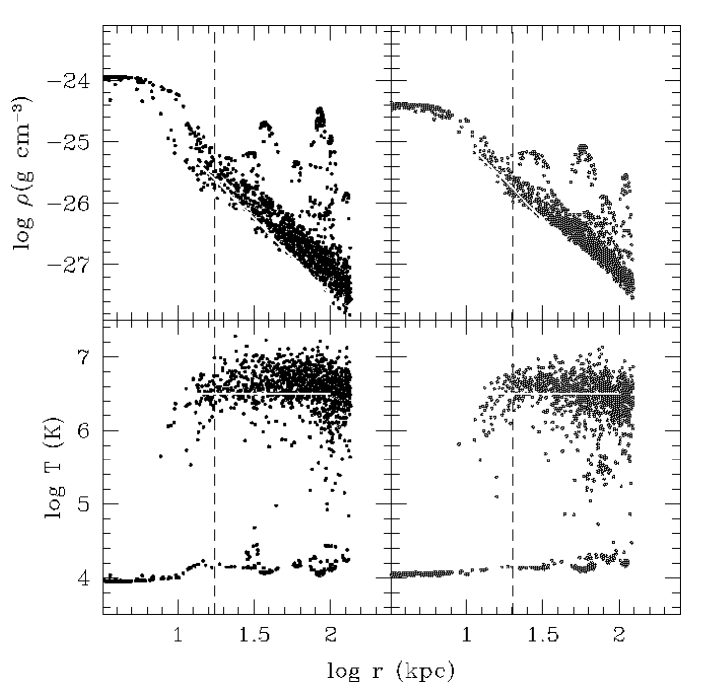
Figure 5: Comparison of gas density (top panels) and temperature (bottom panels) between APMSPH (left panels) and HYDRA (right panels) for a halo of mass $5\times 10^{12}M_{\odot}$ in the 22-64-k simulations at $z=2.33$. The APMSPH halo has higher density in the centre and also in the in-falling satellites. Thick lines are the same in the left and right panels and were drawn to guide the eye. The vertical dashed line denotes the gravitational softening, the SPH smoothing length $h$ is at least half that.

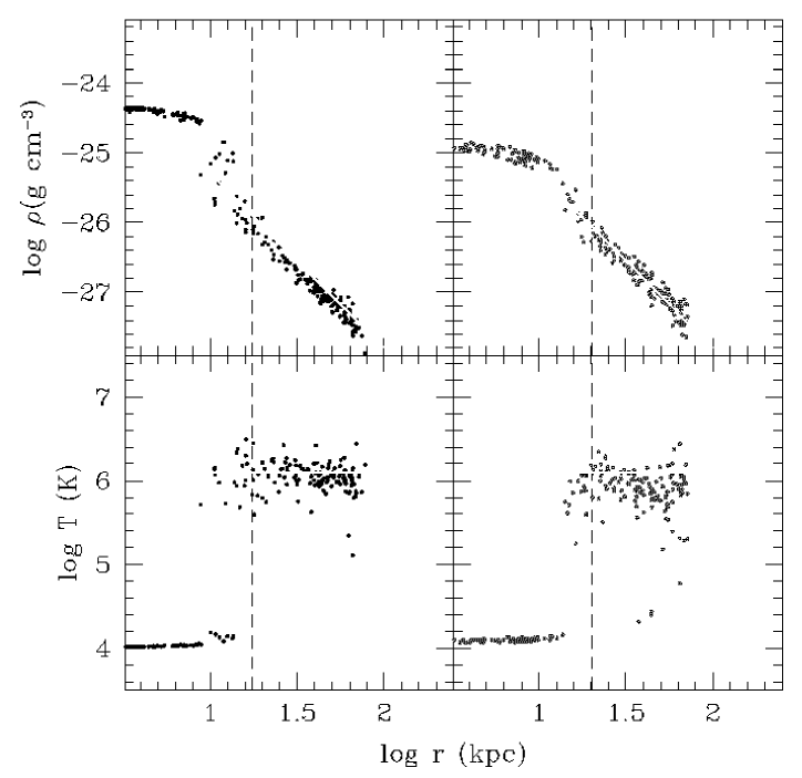
Figure 6: Same as figure 5 but for a halo of mass $5\times 10^{11}M_{\odot}$.

Figure 7: Same as figure 5 but for a halo of mass $5\times 10^{10}M_{\odot}$.

3.2 Spectra

To compare the statistics of simulated spectra with those presented by Hernquist et al. (1996), we will use in this section both their initial conditions and their cooling rates (our runs A-22-64-k and H-22-64-k). These simulations should, in principle, use the spectral evolution of Haardt & Madau (1996) but with a reduced amplitude (see Table LABEL:table:runs), for which we give the fits to the ionising spectrum in Appendix B. Unfortunately, the actual evolution of the background radiation is not identical, since there were small changes between the fit to $J_{21}(z)$ in the preprint of Haardt & Madau (1996), from which Hernquist et al. took their evolution, and the one which appeared in print (D. Weinberg, private communication).

This Section is organised as follows. We begin by comparing spectra along a given line of sight between APMSPH and HYDRA . Next, we compare global spectral measurements (mean absorption and one-point distribution of the optical depth). Finally, we compare spectral statistics (column- and $b$-parameter distributions) deduced from automated Voigt-profile fitting of lines. Our detailed description of the calculation of simulated spectra is given in Section A.4.

3.2.1 Individual spectra

We have computed absorption spectra through the middle of the computational box of the 22-64-k simulations at a redshift of $z=2.33$. Figures 8–10 compare the results of APMSPH with HYDRA , showing simulated spectra, density, temperature and peculiar velocity along a particular line of sight. These figures show that maxima in the density distribution give rise to increased absorption with line widths determined by Doppler broadening and Hubble expansion, as also shown by previous authors. For hydrogen there are regions with very low absorption making a distinction between ‘lines’  and continuum possible, but this is no longer true for helium nor for hydrogen at higher redshifts. The agreement between the two codes is impressive, both for ${\rm H{\sc i}~{}}$and ${\rm He{\sc ii}~{}}$as well as for the total density, over most of the velocity range. The excellent agreement increases our confidence that both codes are working properly and can be used to study the Lyman-$\alpha$ forest.

Figure 8: Absorption spectrum for ${\rm H{\sc i}~{}}$through the middle of the box of the 22-64-k simulation at $z=2.33$. From top to bottom: ${\rm H{\sc i}~{}}$absorption spectrum, ${\rm H{\sc i}~{}}$fraction, ${\rm H{\sc i}~{}}$weighted temperature, ${\rm H{\sc i}~{}}$weighted peculiar velocity. The top graph is versus velocity (wavelength), the bottom three graphs are in units of position along the line of sight, from the front of the box to the back. Solid lines refer to APMSPH simulation, dashed lines to HYDRA .

Figure 9: Same sight line as in figure 8 but now showing ${\rm He{\sc ii}~{}}$results.

Figure 10: Comparison of the state of the IGM between APMSPH (full lines) and HYDRA (dashed line) along the same line of sight as figures 8 and 9, showing gas density, temperature and peculiar velocity (from top to bottom, respectively) versus position in the box. Density is in units of the average gas density at that redshift.

3.2.2 Global spectral characteristics

We have computed simulated spectra along 1024 lines-of-sight on a square grid through the box of the 22-64-k simulations at various redshifts. From the spectra we have computed the effective mean optical depth at this redshift, $\bar{\tau}(z)\equiv-{\rm ln}(\sum_{1}^{N_{p}}e^{-\tau}/N_{p})$ where the sum is over $N_{p}$ pixels of the spectrum. Figure 11 shows that APMSPH , HYDRA and TREESPH predict a very similar redshift evolution for $\bar{\tau}(z)$. Most of the remaining differences are presumably due to the slightly different assumed evolution of the background flux, as can be seen by comparing the HYDRA*and TREESPH* curves. The latter runs use identical fits to the photo-ionising flux although they still use a different fit to the photo-heating rates. A more detailed comparison is shown in figure 12 which depicts the one-point probability distribution for the optical depth in a pixel. Again the comparison is satisfactory, with most of the difference between the Tree and the P3M codes being due to the different background flux. Note that the apparent shift in the mean of $P(\tau)$ between Tree and P3M codes is not just due to the difference in $\bar{\tau}$. Indeed, when the distribution of $P(\tau/\bar{\tau})$ is plotted as in figure 13 then some differences remain, indicating that also the shape of $P(\tau)$ is not quite the same between the codes. The APMSPH & HYDRA codes show small differences in the high $\tau$ tail, which is a consequence of the small differences in the properties of the high density gas, as we remarked on earlier.

Figure 11: Mean effective optical depth $\tau$ as a function of redshift $z$ for runs A-22-64-k & H-22-64-k and published data from TREESPH . The top panel refers to hydrogen, the bottom panel to singly ionised helium. The APMSPH & HYDRA curves are computed from $32^{2}$ sight lines through the box. The TREESPH data were taken from figure  3 in Croft et al. (1997). The HYDRA*and TREESPH* use the fit equations. 3-5 from Croft et al. (1997) for the evolution of the ionization rate divided by two, the other two use the fit from table 4, divided by two.

Figure 12: One-point probability distribution of optical depth for ${\rm H{\sc i}~{}}$(open symbols) and ${\rm He{\sc ii}~{}}$(filled symbols) for the same simulation as shown in figure 11 at a redshift of $z=2.33$. Symbols: APMSPH : circles; HYDRA : squares; TREESPH : triangles. The APMSPH and HYDRA curves assume the fit in Table 4 for the background radiation; the TREESPH data were taken from figure 11 in Croft et al. 1997.

Figure 13: Same as figure 12 but for probability distribution of the ${\rm H{\sc i}~{}}$optical depth in units of the mean.

3.2.3 Voigt-profile analysis

In the previous sections we have shown that APMSPH and HYDRA spectra along a given line of sight look very similar and that global statistical quantities of the optical depth distribution are similar as well. Here we want to compare the statistical properties of the simulated absorption lines based on Voigt profile (VP) fitting. VP fitting has consistently been used to analyse the complex blended features of the Lyman-$\alpha$ forest, seen in real quasar spectra (e.g. Webb 1987, Carswell et al. 1987) and in numerical simulations (Davé et al. 1997, Haehnelt & Steinmetz 1998, Zhang et al. 1998). The technique was devised initially under the premise that the forest lines arose from discrete absorbing clouds intervening the quasar line of sight, a picture currently challenged by the successful reproduction of such observed VP parameter distributions by the smoothly distributed IGM naturally occurring within gas-dynamical simulations.

As we have seen earlier, many of the ‘lines’  occurring in these simulations have significant distortions from the simple Voigt profile due to the fact that the structure giving rise to the line is extended in space and thus still takes part in the Hubble expansion. VP-fitting of such a system then requires a complex blend of several Voigt profiles with a range in column density and velocity width. Consequently, the parameters characterising these components cannot automatically be used to infer physical properties of the absorbers. Given the loss of a physical justification for the VP approach, the method serves merely as way of characterising the undulations of what has been described more accurately by authors as a Lyman-$\alpha$ Gunn-Peterson-effect (Gunn & Peterson 1965). Its power as a diagnostic tool for doing this must be scrutinised, before agreement with the observations can be described as a success for the model. However, since we want to compare our simulated spectra with observed ones, it is important that we analyse them in the same way. We therefore use a standard package for VP fitting (Carswell et al. 1987) used frequently by observers. We will also show that the results deduced from VP-fitting are relatively insensitive to the detailed implementation of the profile fitting. There is however one remaining difference between the simulated and real spectra, namely our simulated spectra are not superposed onto the continuum of a background quasar. It is therefore difficult to model the continuum fitting performed by observers. This problem is aggravated by the small length of our simulated spectra compared to observed ones. We try to estimate the uncertainty introduced by this below.

In this paper, we use an automated version of the VPFIT software (Carswell et al. 1987) written to perform $\chi^{2}$ minimisation over many VP parameters given observational spectra. Prior to using VPFIT, each spectrum is convolved with a Gaussian profile with FWHM = 8 km s^-1, then re-sampled onto pixels of width 3 km s^-1 to mimic the instrumental profile and characteristics of the HIRES spectrograph on the Keck telescope, which currently provides the most up-to-date results on the properties of the weak Lyman-$\alpha$ forest lines. Artificial noise is introduced by adding a Gaussian random signal with zero mean, and standard deviation $\sigma=0.02$ to every pixel (i.e. a SNR of 50 for pixels at the continuum), mimicking the read-out noise dominated character of modern observed spectra.

In our simulated spectra, zero-order absorption occurs across each line of sight that would presumably be removed during observational analysis by the continuum fitting procedure. In analysing real spectra, the continuum is normally determined by fitting a low-order polynomial to apparently ‘unabsorbed’  regions of the spectrum that are typically much longer than our simulated spectra. This difference in spectral range means that we cannot mimic the continuum fitting procedure used by observers on our simulated spectra. The observational procedure depends a great deal on the quality of data as well as on redshift since finding ‘unabsorbed’  regions of the spectrum becomes more difficult at higher redshift, where the Lyman-$\alpha$ forest opacities are higher. Our spectra cover a small enough velocity range to be fit by a flat continuum, as chosen by a simple procedure described as follows. A low average continuum level is assumed initially, then all pixels below and not within 1 $\sigma$ of this level are rejected, and a new average flux level for the remaining pixels is computed. The same condition is applied for this new level and so-on, until the average flux varies by less than 1% (note that the signal to noise ratio adopted is 50 at the continuum). This final average flux level is adopted as the fitted continuum, and the spectrum is renormalised accordingly. We test for the effects of varying this level on the VP results (see below).

The final stage in preparing spectra for VPFIT is via an automatic procedure to find first guess profiles for each line. We make initial guesses using the method of Davé et al. (1997) for finding weak lines, i.e. firstly smoothing the spectrum before ‘growing’  a Voigt profile into the deepest depression. We repeat this procedure on the spectrum with the current best fit Voigt profile subtracted, until the residual absorption varies by less than 20%. VPFIT turns out to be robust in finding accurate fits given few and even quite wrong initial guesses, so we are confident that our results do not depend strongly on the details of the procedure for obtaining first guesses. VPFIT then uses these guesses to find the best-fitting profiles, adding more lines and removing ill-constrained lines where necessary. In general, we calculated VP parameters for a spectrum until an overall reduced $\chi^{2}$ value for the fit falls below 1.3, unless otherwise indicated. This is carried out for typically 300 sight line spectra taken on a grid through each simulation. We check below the effects of varying the required minimum reduced $\chi^{2}$ value.

It is not clear a priori that the deduced VP statistics are independent of the fitting procedure, given e.g. the non-uniqueness of Voigt profiles in fitting a blended line and the fact that observers often fit profiles by hand. Nevertheless, we will show below that our deduced statistics are in excellent agreement with the ones obtained by Davé et al. (1997), using an independent fitting procedure.

In figure 14 we show the column density distribution (the number $N$ of lines per unit redshift and column density $d^{2}N/dz/d\log N_{\rm H{\sc i}}$, or ‘differential distribution function’ , DDF) for runs 22-64-k which use the initial conditions from Hernquist et al. (1996) undertaken using APMSPH (solid), and HYDRA (dotted) at redshift 2. Also shown are the results of a second similar simulation using APMSPH (dashed), but where the initial conditions are drawn from a different random realization of the initial density field (run A-22-64). All three simulations produce very similar DDFs across the range of column densities $\leq 10^{15}$ cm^-2. There is good agreement between the two codes at $z=3$ as well, as illustrated in figure 15. It is gratifying to conclude that these results should not depend greatly on either our code implementations, nor the specific realization chosen, nor the VP-fitting procedure as applied to two different sets of spectra at both redshifts.

Superposed on the simulated DDFs are observationally determined points of Petitjean et al. (1993, hereafter PWRCL) and Kim et al. (1995, hereafter KHCS) for redshift $z=2.0$ and 2.3, and Hu et al. (1995, hereafter HKCSR), for $z=3$. We see that the simulations follow the observed points well, though possibly under predicting lines with $N_{\rm H{\sc i}}>10^{13}$ cm^-2 at $z=2$. More importantly however, our simulated DDFs are directly comparable to the derived column density distributions of figures 2 and 3 of Davé et al. (1997) where the same cube simulated using TREESPH was analysed in a similar way using the AUTOVP/PROFIT fitting software, instead of VPFIT. We find that there is a very close similarity. The results of Davé et al. at $z=2$ also under predict the points of PWRCL and have a very similar slope to our DDF for $N_{{\rm H{\sc i}}}>10^{13}$ cm^-2. Further at $z=3$, the distribution lies constantly above the $z=2$ results for $N_{{\rm H{\sc i}}}>10^{13.5}$ cm^-2, but has a shallower slope at lower column densities. The exact comparison for $N_{{\rm H{\sc i}}}<10^{13.5}$ cm^-2, as shown later, is sensitive to the VP-fitting conditions, nevertheless the similarity is striking enough to suggest that the detailed nature of the weak Lyman-$\alpha$ forest column density distributions are reproducible given both different simulation codes and VP-fitting software.

Figures (16-17) show the derived $b$-parameter distributions for each simulation described above. We follow Davé et al. (1997) and include only lines with $N_{\rm H{\sc i}}>10^{13}$ cm^-2 to eliminate broad, weak features, which are sensitive to the VP-fitting process, from biasing the comparison with observations. These distributions show a consistency indicating independence with simulation code and realization. The shape of the $b$ parameter distribution is very similar to the one obtained by Davé et al. (1997, see their figure 3), from their analysis of TREESPH simulations with the same initial conditions and resolutions as our A-22-64-k and H-22-64-k runs. However there is a clear discrepancy between the observed $b$ distribution as determined by HKCSR at $z=3$ from observations and the simulation results at that redshift. Our simulations all over-predict lines with $b<20$ and $b>50$ km s^-1, whilst failing to reproduce the observed high peak of lines at $b\sim 30$ km s^-1. Although the $b$ parameter distribution is sensitive to the signal to noise ratio and the VP set-up, we will show below that the dominant reason for the discrepancy with observations is lack of numerical resolution.

Figure 14: Column density distributions, $d^{2}N/dz/dlogN_{\rm H{\sc i}}$, from an analysis using VPFIT of 300 spectra along lines of sight through several 22Mpc, $64^{3}$ particle simulations, at $z=2$. Solid and dashed lines show results of A-22-64-k, and H-22-64-k simulations respectively, run using the same initial conditions as used by Hernquist et al. (1996) (c.f. figure 2 of Davé et al. 1997). The dotted line shows results of an APMSPH simulation run with different initial conditions (A-22-64). Observational results of PWRCL and KHCS with mean absorption redshifts $\bar{z}=2.0$ and 2.3 respectively, are also plotted as indicated.

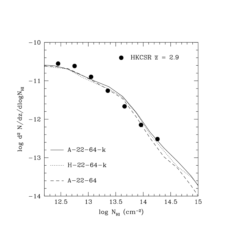
Figure 15: Same as figure 14 but at $z=3$. Observational results of HKCSR with mean absorption redshifts $\bar{z}=2.9$ are plotted.

Figure 16: $b$-parameter distributions correspondoing to the column densities shown in figure 14. Only lines with $N({\mbox{${\rm H{\sc i}~{}}$}})>10^{13}$ cm^-2 are included.

Figure 17: $b$-parameter distributions corresponding to the column densities shown in figure 15. Only lines with $N({\mbox{${\rm H{\sc i}~{}}$}})>10^{13}$ cm^-2 are included. The histogram shows the corresponding observational results of HKCSR.

4 Numerical effects

In the previous section we have shown that there is excellent agreement between APMSPH , HYDRA and TREESPH on a variety of statistics that characterise the simulated Lyman-$\alpha$ spectra. The different codes, however, were compared at identical numerical resolution. In this section, we will investigate how sensitive these statistics are to details of the simulation and analysis, such as numerical resolution, box size, and details of the VP-fitting process. To investigate the effects of numerical resolution one would ideally like to do a simulation of a given region of space at several resolutions to asses the degree of convergence. However, since the required CPU time to perform a given simulation rapidly increases with the number of particles in the run, we have opted to keep the number of particles fixed but decrease the box size. This complicates the analysis since differences in statistics between a small and a large box may be due to the lack of long wavelength perturbations and saturation of modes in the smaller box, rather than non-convergence of the simulation in the larger box. In the same vein as the previous section we will describe first how global properties depend on resolution before concentrating on line statistics. We will then investigate the dependence of line statistics on the VP-fitting procedure. Finally, we will investigate how line statistics depend on the assumed UV background.

4.1 Numerical resolution

4.1.1 Global spectral characteristics

We have computed the effective mean optical depth $\bar{\tau}(z)$ at various redshifts as well as the one-point probability distribution $P(\tau)$ from 1024 lines-of-sight for the A-22-64, A-11-64 and A-5-64 simulations. Figure 18 shows only small differences for the $\bar{\tau}_{\rm H{\sc i}}$ optical depth as the resolution is increased. Note that the optical depth tends to decrease with increasing resolution. The main reason for this is that at higher resolution, small halos collapse that were not resolved at lower resolution. This decreases the density of gas in the low density regions which leads to a decreasing optical depth. This effect is much more pronounced for helium, for which there are still significant differences in mean optical depth between A-11-64 and A-5-64. Note that this is a resolution and not a box size effect: the A-5-32 box also shown in the figure has the same resolution as the A-11-64 box and gives the same optical depths despite its different box size. We have therefore run an even higher resolution simulation, A-2.5-64, which gives a mean optical depth for ${\rm He{\sc ii}~{}}$at $z=4$ of $\bar{\tau}=2.63$ which is reasonably close to the value 2.78 of the A-5-64 simulation. This suggests that the ${\rm He{\sc ii}~{}}$absorption has almost converged in our highest resolution simulations, but not in the lower resolution ones.

Zhang et al. (1997) already pointed out that it is far more difficult to obtain convergence for the effective mean optical depth for helium than for hydrogen. To explain the reason for this we first define the effective mean optical depth $\bar{\tau}(\rho)$ at given density $\rho$ from

$$\exp(-\bar{\tau}(\rho))=\sum\exp\left(-\tau(\rho)\right)/N(\rho)\,,$$ (3)

where the sum is over all $N(\rho)$ pixels in the simulated spectra where the real space density in the particular pixel is $\rho$ (see e.g. the discussion of figures 6c & 6d in Croft et al. 1997). For later use we define the normalised volume fraction of gas at density $\rho$ as $P(\rho)=N(\rho)/N_{p}$, where $N_{p}$ is the total number of pixels. Now, at higher resolution a larger fraction of gas collapses into halos with a modest over density which are simply not resolved in lower resolution simulations. At $z=2$ for example, this reduces the fraction of gas at densities $\sim(0.1-1)\times\bar{\rho}_{B}$ and correspondingly increases that fraction at densities $\sim(1-10)\times\bar{\rho}_{B}$, as is illustrated in figure 19, where we show the distribution of cool and hot gas (as defined in Section 3.1.1) at each resolution. The gas that collapses to higher densities has an effective mean optical depth $\lower 2.15277pt\hbox{\mbox{$\;\buildrel<\over{\sim}\;$}}1$ in hydrogen yet $\tau\gg 1$ for helium, as is also shown in the figure. Therefore, for hydrogen some of the absorption lost because of the decreased fraction of low density gas is recuperated from the increased opacity in the higher density gas. This is not true for helium, however, since the lower density gas is already optically thick and increasing its column density does not significantly change its net absorption. The same reasoning applies at higher redshifts where it is even clearer that the amount of cool gas is resolution dependent and has only just converged in our highest resolution simulation. Miralda-Escudé (1993) previously remarked that for a large jump in ionising flux from the ${\rm H{\sc i}~{}}$limit to the ${\rm He{\sc ii}~{}}$limit, as occurs in the Haardt & Madau (1996) spectra, lines with an ${\rm H{\sc i}~{}}$column density of $\sim 10^{12}$ cm^-2 have central ${\rm He{\sc ii}~{}}$optical depths $\sim 1$. Hence for a simulation to have a reliable ${\rm He{\sc ii}~{}}$mean effective optical depth it needs to resolve well lines with ${\rm H{\sc i}~{}}$column density of $\mbox{$\;\buildrel<\over{\sim}\;$}10^{12}$ cm^-2. We will show later (figure 21) that the A-22-64 simulation produces far fewer lines with such low column densities than the higher resolution runs, which then explains why the low resolution simulation has a considerably higher mean effective ${\rm He{\sc ii}~{}}$optical depth.

We have shown in figure 19 that the amount of cool gas is strongly resolution dependent. In particular, run 22-64-k, which has identical parameters and resolution to the Hernquist et al. (1996) simulation, underpredicts the amount of cool, high density gas by a large fraction (a factor of $\sim 5$ at $z=3$). Since lines of sight intersecting high density cool gas regions produce damped Lyman-$\alpha$ absorbers, the statistics of those damped Lyman-$\alpha$ systems, as deduced from these simulations (Katz et al. 1996a), are uncertain because they are very sensitive to numerical resolution.

Figure 18: Mean effective optical depth $\bar{\tau}$ as a function of redshift $z$ for several box sizes indicated in the figure. The top panel refers to hydrogen, the bottom panel to singly ionised helium. The $64^{3}$ simulations have mass resolutions of $1.4\times 10^{8}$, $1.8\times 10^{7}$, $2.2\times 10^{6}$ and $2.1\times 10^{5}M_{\odot}$ per SPH particle, respectively.

Figure 19:

Mass fractions at given density in the hot and cool phases for various redshifts for runs A-22-64 (full lines), A-11-64 (long dashed) and A-5-64 (short dashed) for various redshifts as indicated in the panels (see Section 3.1.1 for definition of cool/hot). At higher resolution a larger fraction of gas collapses to higher densities leading to less gas at densities $\rho\sim(0.1-0.3)\times\bar{\rho}_{B}$ which contributes most to the absorption. The symbols in the $z=5$ panels refer to our highest resolution A-2.5-64 run and compare well with the lower resolution A-5-64 run. The dot-dashed lines in the cool gas panels at $z=3$ and $z=2$ indicate the effective mean optical depth $\bar{\tau}(\rho)$ as a function of density measured from the simulations for hydrogen and helium (curve giving higher values, right scale).

Figure 20: Mean transmission at given density, $1-\exp(-\bar{\tau}(\rho))$, weighted by the fraction by volume of pixels $P(\rho)$ at that density, plotted versus density, illustrating which densities contribute most to the absorption as a function of redshift, indicated in the panels. Full curves: A-22-64, dashed curves: A-5-64, for hydrogen (thick lines) and helium (thin lines).

The influence of resolution on optical depth is further illustrated in figure 20 which compares the net transmission of gas as a function of its density for our highest and lowest resolution runs. The figure illustrates clearly that at higher resolution the transmission in the low density gas increases significantly but for hydrogen this is mostly compensated by a decrease in transmission in the higher density pixels. This compensation does not happen for helium and consequently the helium optical depth decreases noticeably with increased resolution. Note also that, although the hydrogen mean optical depth has converged there are still significant differences in the distribution of $P(\rho)\,(1-\exp(-\bar{\tau}(\rho)))$.

4.1.2 Line statistics

Figure 21: Column density distribution dependence on box-size and resolution at z=2. Results are shown for three simulations run using APMSPH with the same initial modes, but with box size and particle numbers as indicated. Observational results of KHCS and PWRCL are also plotted as indicated.

Figure 22: Corresponding $b$ parameter distributions to the column densities shown in figure 21 for lines with $N_{h}>13$ cm^-2, at $z=2$. The histogram shows the corresponding observational results of KHCS. Note that the highest bin plotted for the KHCS results contains only 18 lines.

Figure 23: Same as figure 21 for $z=3$. Observational results are taken from KHCS and HKCSR, using independent data.

Figure 24: Same as figure 22 for $z=3$. The histogram shows the observational results of HKCSR.

We have used VP-fitting with the set-up as described earlier to characterise the absorption lines in simulated spectra to investigate the extent to which VP distributions depend on numerical resolution. The results are shown in figures 21-24 for redshifts 2 and 3. The number of hydrogen lines with column density $\geq 10^{13}$ cm^-2 is largely independent of resolution and box size at both redshifts, as shown by the DDFs in figures 21 and 23, which is quite encouraging. However below this column density, the lower resolution simulation A-22-64 starts to lose a significant number of lines. The higher resolution simulations show excellent agreement with the observed DDFs also indicated in the figures for both redshifts, although there may be a hint that the simulations underproduce lines at redshift 2.

This agreement does not extent to the $b$-parameter distributions however. Simulations at different resolutions produce quite different $b$-parameter distributions, none of which fit particularly well the observed one. Higher resolution simulations produce a larger fraction of narrower lines. Note that the $b$-parameter distributions shown in the figures are restricted to lines with $N_{\rm H{\sc i}}\geq 10^{13}$ cm^-2 where there was good agreement for the DDF between simulations at different resolution. We will show in the next section that these $b$-parameter distributions are in fact also quite sensitive to the parameters used in the VP-fit analyses (e.g. required reduced $\chi^{2}$ and continuum placement), complicating the comparison with observational data.

4.2 Dependence on VP-fitting procedure

Figure 25: Column density distributions derived from the same A-11-64 simulation at $z=2$ but varying the reduced $\chi^{2}$ requirement and continuum level chosen for each spectrum. Solid and dotted lines show results requiring the overall VP-fitting to each spectrum to have a reduced $\chi^{2}<1.3$ and 2 respectively. Short-dashed and long-dashed lines show the effect of respectively raising and lowering the chosen continuum fit for each spectrum by 2%, prior to VP-fitting, for $\chi^{2}<1.3$. Observational results of KHCS and PWRCL are also plotted as indicated.

Figure 26: $b$-parameter distributions corresponding to the column densities shown in figure 25 for lines with $N_{\rm H{\sc i}}>10^{13}$ cm^-2. The histogram shows the corresponding observational results of KHCS. Lines broader than 100 km s^-1 are arbitrarily set to 100 km s^-1.

The VP-fitting process is sensitive to the quality of the observational data, the continuum level chosen, and the strictness of the fit demanded, as we will quantify here. In figure 25 we show the DDF of the high resolution A-11-64 simulation at z=2, calculated using varying VP-fitting parameters. The solid line shows our previous results obtained using the default reduced $\chi^{2}$ requirement, $\chi^{2}<1.3$, and choosing a continuum fit as described previously. The dotted lines show the results of relaxing the $\chi^{2}$ requirement to $\chi^{2}<2$, thereby simulating observations with lower signal to noise. This clearly reduces the number of very weak lines, $N_{{\rm H{\sc i}}}<10^{12.5}$ cm², found, but otherwise leaves the DDF unchanged. The long-dashed line shows the results when the continuum level found by the procedure outlined above is then lowered by just 2%, this being the noise level set for these spectra (once again requiring $\chi^{2}<1.3$). Here we see a similar but even less noticeable effect. Finally the short-dashed line shows the result of raising the continuum level by the same amount. We see now that the column density distribution is slightly raised down to $N_{{\rm H{\sc i}}}<10^{13.5}$ cm². Beyond this column density it seems that the distribution found is insensitive to the chosen parameters of the VP fitting process.

Figure 26 shows the $b$-parameter results given the different VP analyses described above. Encouragingly, the changes are slight except for the case where the continuum level is chosen higher which decreases significantly the height of the observed peak and correspondingly increases the number of lines at large values of $b\geq 100$ km s^-1.

4.3 Comparison with UV background scaling

Figure 27: Column density distributions derived from H-11-64-j simulations at z=2. The solid and dot-dashed lines show results where the assumed UV backgrounds are given by HM/2 (tabulated UV background of HM with amplitude divided by 2), and a fixed power-law ($J_{21}=0.5,\alpha=1$), respectively both during run-time and for the calculation of spectra. Results are also shown for the latter simulation but where an HM/2 UV background is assumed for the calculation of spectra (dashed line), and where the original results have been raised by $\log(2.36)$ (dotted line). The latter factor 2.36 is the ratio of the flux at the Lyman-$\alpha$ limit between the $J_{21}=0.5$ power law spectrum and the HM/2 one. Observational results of KHCS and PWRCL are also plotted as indicated.

Figure 28: $b$-parameter distributions corresponding to the column densities shown in figure 27 for lines with $N_{\rm H{\sc i}}>10^{13}$ cm^-2. The histogram shows the corresponding observational results of KHCS.

The deduced DDFs and $b$-parameter distributions depend on the amplitude of the assumed ionising background which is not well known, and on the baryon fraction which is equally uncertain. The shape of the radiation spectrum also determines the amplitude and slope of temperature-density relation obeyed by the cool IGM (see equation (65) for the case of a power law radiation spectrum) and hence has some influence on the neutral fraction of gas at a given density. This potentially introduces a large parameter space to search through with numerical simulations. Fortunately, the resulting optical depth only depends on a particular combination of these parameters. Indeed, in ionization equilibrium the number of photo ionizations per unit time balances the number of recombinations, hence $J_{21}\rho\propto\alpha_{\rm H{\sc ii}}\rho^{2}$. The recombination coefficient scales with temperature as $\alpha_{\rm H{\sc ii}}\propto T^{-0.7}$, so in the low density phase where $\rho\propto T^{1.7}$ we find $\tau\propto\Omega_{B}^{2-0.7/1.7}/J_{21}\propto\Omega_{B}^{1.59}/J_{21}$ (e.g. Hui & Gnedin (1997) and Appendix C for details). The exponent of $\Omega_{B}$ depends weakly on the shape of the ionising spectrum. We now show that simulations can be run with one set of values of $\Omega_{B}$ and $J_{21}$ and later scaled to good accuracy to another set. Figure 27 compares the DDFs for simulations H-11-64 and H-11-64-j. The first of these was run with the Haardt & Madau (1996) ionising background (with amplitude divided by 2, indicated by the lines labelled ‘HM/2’ ) and the second with an imposed power law spectrum of ionising photons with constant amplitude $J_{21}=0.5$ and slope $\alpha=1$. The DDFs of these two runs are significantly different, with the H-11-64 run producing more lines at all column densities. However, if we assume in the analysis phase that the spectrum is HM/2 for the H-11-64-j run than we obtain an almost identical DDF as for the original H-11-64 run. This kind of scaling also works well for the associated $b$-parameter distributions, shown in figure 28. Note that the run with power law ionising sources produces a $b$-parameter distribution very similar to the original HM/2 run, even without post-processing scaling.

5 Comparison with observations

Figure 29: Mean optical depth $\bar{\tau}$ as a function of redshift $z$ for our highest resolution run A-5-64 (open squares connect by solid line). The top panel refers to hydrogen, where we have plotted the observed data points presented in Rauch et al. (1997) and those determined by Fardal et al. (1998, denoted FGS) using combined line-lists from authors using high-resolution spectra. The bottom panel refers to singly ionised helium. The observational data points shown are those of Davidsen et al. (1996, DKZ), Jakobsen (1997, BDGJP), Reimers et al. (1998, RKWGRW) and Tytler et al. (1998, as plotted in figure 1 of Fardal et al. 1998). The dashed line connecting triangles in the lower panel shows the effect of increasing the $\Gamma_{\rm H{\sc i}}/\Gamma_{\rm He{\sc ii}}$ break in the Haardt & Madau UV background by a factor 2.

Figure 30: $b$-parameter distribution for lines with $N_{\rm H{\sc i}}>10^{13}$ cm^-2 at $z=4$ for A-5-64 and A-2.5-64 compared to data from Williger et al. (1994) and Lu et al. (1996). These two data sets were taken with different resolution and so we analysed the simulated spectra accordingly: A-5-64-Williger is analysed assuming a FWHM of 12 km s^-1 and SNR of 20 in the VPFIT procedure, A-5-64-Lu and A-2.5-64-Lu with FWHM of 8 km s^-1 and SNR of 60.

Figure 31: $b$-parameter distribution for lines with $N_{\rm H{\sc i}}>10^{13}$ cm^-2 for A-5-64, after increasing the temperature of all gas arbitrarily by a factor of two, for redshifts 4, 3 and 2 (top to bottom respectively). The VPFIT parameters in the analysis were chosen to allow comparison with the data of Lu et al. (1996, $\bar{z}=3.9$), Hu et al. (1995, $\bar{z}=2.9$) and Kim et al. (1997, $\bar{z}=2.3$), which are superposed for comparison.

Given the level of convergence of simulated quantities, as discussed in the previous section, we now turn our attention to a detailed comparison of simulations with observations at redshifts $\geq 2$.

A comparison of the effective optical depths for ${\rm H{\sc i}~{}}$and ${\rm He{\sc ii}~{}}$, computed from the A-5-64 run at z=2, with observational data is given in figure 29. For the evolution of $\tau_{\rm H{\sc i}}$ we plot the recent results of Fardal et al. (1998), who used a combined line-list from a variety of authors for which only those originating from studies carried out using the HIRES spectrograph on the Keck were included here. We also show the effective optical depths observed by Sargent & Barlow (published in Rauch et al. 1997). It is clear that the simulated $\tau_{\rm H{\sc i}}$ results fit well, as might be expected from the good fit of the ${\rm H{\sc i}~{}}$DDF results. Rauch et al. (1997) used the good agreement between simulated and observed optical depths to set a lower limit on the baryon fraction, using a lower limit on the ionization flux deduced from the observed quasar luminosity function. Since we confirm their simulation results for standard CDM models, we also confirm their lower limit, $\Omega_{B}h^{2}\mbox{$\;\buildrel>\over{\sim}\;$}0.017$.

For $\tau_{\rm He{\sc ii}}$ we have used the recent ${\rm He{\sc ii}~{}}$Gunn-Peterson effect detections collected by Fardal et al. (1998) (see references therein). Although the available $\tau_{\rm He{\sc ii}}$ observations are limited, the results of Davidsen et al. (1996) do supply a strong constraint at $\bar{z}_{\rm abs}=2.4$. In this case our result that the $\tau_{\rm He{\sc ii}}$ value inferred from our simulations does indeed change significantly when simulating at higher resolution, means that this constraint is not matched by our simulations which predict a $\tau_{\rm He{\sc ii}}$ lying about a factor 2 below the observed value. Unlike the conclusions of Croft et al. (1997) we consequently find it is impossible to match both the $\tau_{\rm H{\sc i}}$ and the $\tau_{\rm He{\sc ii}}$ observational constraints by a applying a single renormalisation to the Haardt & Madau (1996) UV background spectrum, and instead require a ’softer’ spectral shape. Since $\tau_{\rm He{\sc ii}}$ scales as $\tau_{\rm He{\sc ii}}/\tau_{\rm H{\sc i}}\propto\Gamma_{\rm H{\sc i}}/\Gamma_{\rm He{\sc ii}}\propto J_{\rm H{\sc i}}/J_{\rm He{\sc ii}}$, where $J_{\rm H{\sc i}}/J_{\rm He{\sc ii}}$ is the ratio of the ionising flux at the respective ${\rm H{\sc i}~{}}$and ${\rm He{\sc ii}~{}}$limit frequencies, we can increase the helium optical depth by scaling the helium ionization rate keeping the hydrogen photo-ionization rate constant. Increasing the ratio $J_{\rm H{\sc i}}/J_{\rm He{\sc ii}}$ by a factor two at all observable redshifts from $\sim 7$ to $\sim 14$ then provides a good fit to both the ${\rm H{\sc i}}$ and ${\rm He{\sc ii}}$ optical depths (figure 29).

This softened UV background may yet prove to be consistent with the UV background inferred from quasars alone, since recent estimates of the ‘average’  intrinsic quasar spectral index have yielded softer values $\sim 1.8$ (Zheng et al. 1997), as opposed to the value $1.5$ originally assumed in Haardt & Madau (1996). Nevertheless, since the values of the UV background at the ionising edges are strongly affected by the self-absorption by Lyman-$\alpha$ forest clouds, we must wait for more detailed models taking these effects into account before drawing any strong conclusions. The values for $\Gamma_{\rm H{\sc i}}$, and $\Gamma_{\rm He{\sc ii}}$ depend somewhat on the effective slope of the spectrum at frequencies immediately higher than their ionising frequencies, however this dependence is weak, so achieving the required factor two change in the ratio of photo-ionising coefficients by changing the background spectrum in this way is unlikely.

Previously we have have shown that our SCDM simulations using the Haardt & Madau (1996) spectrum (with amplitude divided by 2) reproduce the observed DDFs quite well, both at $z=2$ (figure 21) and $z=3$ (figure 23). The only discrepancy may be that the simulations produce a slightly lower DDF than seen at $z=2$ by Petitjean et al. (1992). The difference is slight and in any case the observations are as yet not discriminating enough at this redshift to really suggest that this is a problem, as the newer results of Kim et al. (1997) at $z=2.3$ are somewhat discrepant with the older data. However it is not clear at present to what extent the DDF discriminates different plausible cosmological models and consequently it is not yet possible to use the relatively good agreement between observed and simulated DDFs as an argument in favour of our assumed cosmology.

The simulated and observed $b$-parameter distributions at $z=4$ are compared in figure 30. We have analysed the simulated spectra using a VPFIT set-up that mimics the signal to noise ratio and spectral resolution of the data from Williger et al. (1994, simulations shown as A-5-64-Williger) and Lu et al. (1996, simulations labelled -Lu). For the latter data we compare A-5-64 with the higher resolution A-2.5-64 run. First note the excellent agreement between the different resolution runs, suggesting that the $b$-parameter distribution in the 5Mpc box has very nearly converged. We noted earlier that the ${\rm He{\sc ii}~{}}$optical depth of these two runs is very similar as well, which increases our confidence in the reliability of results drawn from the 5Mpc box run, as far as numerical artifacts such as resolution are concerned. Next note the importance of the wavelength resolution in the analysis stage, by comparing the A-5-64 run analysed with two different VPFIT set-ups. The lower spectral resolution of A-5-64-Williger versus A-5-64-Lu reduces dramatically the peak in the $b$-distribution at $\sim$ 25 km s^-1, correspondingly increasing the number of broader lines. This trend is also shown by the data. The $b$-parameter distribution of A-5-64-Williger provides an excellent fit to the data from Williger et al. (1994), both at low and high $b$ values. At higher resolution, when we compare the A-5-64-Lu curve with the Lu et al. (1996) data, the agreement is still very good. There is however a hint that there are too many narrow lines in the simulated spectra.

This difference between simulated and observed distributions at small $b$-parameters is even clearer at lower $z$ (see figure 22 for $z=2$ and figure 24 for $z=3$, comparing data with the resolved A-5-64 run): the simulated $b$-parameter distributions peak at lower values of $b\sim 20$ km s^-1 whereas the observed ones peak at $b\sim 30$ km s^-1. A fair comparison between observations and simulations is hampered by the sensitivity of the $b$-parameters to the continuum fitting procedure. Note that the high resolution simulations have a box size of only $\sim 10{\mbox{\AA}}$, and this might introduce large continuum errors. Also, the observed $b$-parameter distributions have been shown to vary slightly from quasar to quasar (Kim et al. 1997), though the effect is larger for the higher column density systems $N_{\rm H{\sc i}}>10^{13.8}$ cm^-2. Despite these complicating factors the simplest interpretation of our results is that our simulated IGM has temperatures that are slightly lower by a factor $\sim 2$ than those existing in the actual absorbing IGM. Indeed, if we increase arbitrarily the temperature of the simulated gas by a factor of two (dashed lines in figure 31) then we find excellent agreement between the simulated and observed $b$-distributions at all redshifts 2, 3 and 4, in accord with the findings of Haehnelt & Steinmetz (1998).

What could give rise to such a hotter IGM? As discussed in Section 2.1, the temperature of the IGM at redshifts $z=4\rightarrow 2$ depends on the epoch of reionization. In the Haardt & Madau scenario, ${\rm H{\sc i}~{}}$reionizes at $z\sim 6$ and ${\rm He{\sc ii}~{}}$at $z\sim 4.7$ (dashed line in figure 1b), and the reionization is due to the increase in the combined QSO luminosity at those high redshifts. However, at present there are no known QSOs at $z>5$, hence the assumed increase in QSO flux depends mostly on the extrapolation of the evolution of the QSO luminosity function to higher $z$. If ${\rm He{\sc ii}~{}}$reionization would be delayed, then non-equilibrium effects would give a substantial increase in IGM temperature, even at redshifts of $z\sim 2$. Consequently, uncertainties in the QSO flux at redshifts $\geq 5$ alone would appear to give sufficient leverage for the required increase in the IGM temperature. It is not clear whether such changes in reionization history alone could conspire to give the correct increase in the mean IGM temperature over the whole of the redshift interval $4\rightarrow 2$. Note that any increase in temperature necessary to provide $b$-distributions that fit observations, would in effect scale both the DDF and $\tau_{\rm H{\sc i}},\tau_{\rm He{\sc ii}}$ results further; increasing $T$ by a factor of 2 requires increasing $\Omega_{B}$ by a factor $\sim 2^{0.7}$ to keep the same level of absorption.

There exist some further numerical possibilities that may result in a simulated IGM that appears slightly cool. Firstly, larger waves not included in our highest resolution run of box-size 5.5Mpc could dynamically heat the medium to a greater extent than found in our simulations. The lack of dependence of the $b$-distribution to the different box-sizes examined here indicates that this is probably not an important effect. Secondly, baryons collapsed in small dark matter halos that have formed at high-$z$ could possibly be ‘evaporated’  by a large temperature boost at reionization such as found in the non-equilibrium models. Our smoother temperature increase during reionization may then allow more low-circular velocity halos to capture gas than appropriate. To reiterate then, we find that it is likely that a temperature boost within our simulations is likely to be necessary in order to produce absorption lines that fit the observations at $z=2$, 3 and 4. The necessary temperature increase may well result from a consistent treatment of the thermal history as computed by Haardt & Madau (1996) but including non-ionization equilibrium effects, though our estimates show that higher temperatures due to an even later reionization epoch, may eventually be necessary. Another plausible candidate for extra energy input into the gas is feedback from star formation. Certainly it is likely that in future observations of the Doppler parameter distribution of the Lyman-$\alpha$ forest could become an excellent tool in providing constraints on the thermal history of the universe beyond $z=2$.

6 Summary and conclusions

We have presented a new simulation tool, APMSPH , designed to study numerically the formation of structures responsible for the Lyman-$\alpha$ -forest. This code is very fast and treats the low density IGM relatively accurately, allowing increased resolution at little extra simulation time. The IGM is allowed to interact with a time-dependent but uniform background of ionising photons assumed to come from quasars, using the rates suggested by Haardt & Madau (1996). This background heats the low density gas and changes the form of the cooling function at higher densities. The distribution of the gas in the density-temperature plane can be understood from the relative importance of cooling and heating processes, and from the comparison of the appropriate cooling time scale with the Hubble time.

We performed extensive comparisons of the new code with the HYDRA code of Couchman et al. (1995), which was adapted to study this problem as well. The agreement between the two codes is excellent for a wide variety of statistics. The distribution of gas in the $(\rho,T)$ plane is very similar and various statistics on the distribution of halos agree very well. The amount of gas which is able to cool in collapsed halos is similar in the two codes, showing that coding details are not very important in determining this fraction. We are currently analysing several large HYDRA simulations performed on the T3D computer to understand in more detail how resolution affects Lyman-$\alpha$ statistics (the VIRGO consortium, in preparation). Both APMSPH and HYDRA are based on the Lagrangian SPH method, which has high resolution in high density regions. However, since many lines form in low density regions where SPH suffers from low resolution, it would still be very valuable to compare in detail with some of the Eulerian codes used by other groups.

We also compared our new code with published results from TREESPH (Hernquist et al. 1996) for simulations started from their initial conditions and confirm their findings. We have also analysed independently our simulated spectra from these runs using a different implementation of automated Voigt profile fitting (VPFIT, Carswell et al. 1987). The deduced line statistics in terms of column density and $b$-parameter distributions agree well with their published values, showing that Voigt profile fitting gives reproducible results.

We have then used APMSPH to study the effects of lack of numerical resolution on quantities deduced from simulated spectra based on Voigt profile fitting. The mean effective hydrogen optical depth is converged in our medium resolution simulation and so are the derived column density distributions (DDFs). The latter also are in good agreement with DDFs deduced from observations, for our assumed background flux and baryon fraction. However, the relative amounts of cool gas are rather different when comparing the A-22-64 with the A-11-64 run, which has eight times better mass resolution, and there are still noticeable differences with our highest A-5-64 run (which has another factor of eight better mass resolution), due to lack of numerical resolution. With increasing resolution, we find that the optical depth decreases, especially for ${\rm He{\sc ii}~{}}$, and that the number of lines with small $b$-parameter increases. However, from a comparison of the A-5-64 run with an even higher resolution simulation, A-2.5-64, we find that the A-5-64 box is already very close to convergence and we are relatively confident that we can draw reliable conclusions from this simulation. We found that the deduced $b$-parameter distributions are sensitive to the assumed continuum level, a problem which should also influence observations to some extent. The DDFs, on the other hand, are not very sensitive to the exact VP-fitting procedure.

Some previously published results on the ${\rm He{\sc ii}~{}}$forest are unreliable due to lack of numerical resolution. For example at $z=4$, the mean effective ${\rm He{\sc ii}~{}}$optical depths are 4.54, 3.52, 2.78 and 2.63 for runs A-22-64, A-11-64, A-5-64 and A-2.5-64, respectively. This shows that the required resolution to get the mean optical depth correct is very high. We interpreted the dependence on resolution as being due to the formation of progressively smaller halos being resolved with better resolution. Low density gas falls into these halos and hence the optical depth decreases. The good agreement between the 5.5Mpc and the 2.5Mpc box increases our confidence that these higher resolution runs have effectively converged.

Turning to a comparison of our highest resolution simulation with observations, we come to the following conclusions.

• There is excellent agreement between the observed and simulated Lyman-$\alpha$ column density distributions at $z=2$ and $3$, provided we divide the ionising background intensity advocated by Haardt & Madau (1996) by two, for our assumed baryon fraction of $\Omega_{B}h^{2}=0.0125$. Alternatively, for the intensity of the ionising background as computed by Haardt & Madau, we require a higher baryon fraction (Rauch et al. 1997)

  $$\Omega_{B}h^{2}\mbox{$\;\buildrel>\over{\sim}\;$}0.017\,\,\,\,{\mbox{\rm(from DDFs)}}\,.$$ (4)

• The simulated $b$-parameter distributions peak at lower $b$-values than the observed ones for $z=4$, 3 and 2, suggesting that the simulated IGM temperature in our simulations is too low. We argued that uncertainties in reionization history, combined with non-equilibrium effects and feedback from star formation, might be sufficient to increase the temperature by a factor $\sim 2$, which would bring the simulated distributions into excellent agreement with the observed ones. However, this would increase the required $\Omega_{B}$ even more, since increasing the temperature would decrease the amount of absorption, giving the higher $\Omega_{B}$ limit

  $$\Omega_{B}h^{2}\mbox{$\;\buildrel>\over{\sim}\;$}0.028\,\,\,\,{\mbox{\rm(from $b$-parameter distribution)}}\,.$$ (5)

• The ${\rm He{\sc ii}~{}}$optical depth corresponding to our best fit ${\rm H{\sc i}~{}}$optical depth is lower than observed values, suggesting that the Haardt & Madau ionization spectrum may be too hard. The more recent analysis by Zheng et al. (1997) of observed quasar spectra lead to a similar conclusion. Fitting both ${\rm H{\sc i}~{}}$and ${\rm He{\sc ii}~{}}$optical depths requires a spectral break

  $${J_{\rm H{\sc i}}\over J_{\rm He{\sc ii}}}\approx 14\,.$$ (6)

Overall we find that the level of agreement between simulations of the Lyman-$\alpha$ forest in a scale-invariant, CDM universe and observations, is still impressive. More detailed comparisons between simulations and observations will allow us to study the thermal history of the universe at even higher redshifts.

Appendix A Mathematical description

In the first part of this Appendix we give details of the equations describing the growth of structure. The second part gives the explicit equations for computing SPH quantities in the APMSPH implementation as well as a detailed description of the way we determine SPH neighbours. The third part of this Appendix describes the HYDRA low density correction. In the final part of this Appendix we give the explicit expressions used to compute simulated spectra.

A.1 Physical model

In the Newtonian approximation valid on the scales under consideration, the evolution of structures is governed by the following set of Lagrangian equations:

$${d\hat{\rho}\over dt} = -\hat{\rho}\nabla{\bf x}$$ (7)

$${d\dot{\bf x}\over dt}+2{a\over\dot{a}}\dot{\bf x} = -{1\over a^{3}}\nabla\psi-{1\over a^{2}}{\nabla p\over\rho}$$ (8)

$${du\over dt}+3{\dot{a}\over a}{p\over\rho} = -{p\over\rho}\nabla\dot{\bf x}+\left({1-Y\over m_{H}}\right)^{2}\,\rho({\cal H}-{\cal C})$$ (9)

$$\nabla^{2}\psi = 4\pi G(\hat{\rho}_{\rm T}-\langle\hat{\rho}_{\rm T}\rangle).$$ (10)

Here, $\hat{\rho}\equiv a^{3}\rho$ is the comoving gas density, $Y$ is the helium abundance by mass, ($1-Y$) is the hydrogen abundance, ${\bf x}={\bf r}/a$ are comoving coordinates, ${\bf v}_{p}\equiv a\dot{\bf x}$ is the peculiar velocity, $a(t)=(1+z)^{-1}$ is the scale factor, $t$ denotes time, $z$ is the redshift and $\nabla\equiv\partial/\partial{\bf x}$. The pressure is $p=(\gamma-1)\rho u$, where $u$ is the thermal energy per unit mass and $\gamma=5/3$ for a mono-atomic gas. The density $\hat{\rho}_{\rm T}$ entering in the Poisson equation (10) is the sum of the dark matter and gas density; $G$ is the gravitational constant and $m_{H}$ is the proton mass. The dark matter evolves according to the Euler equation (8) with $p=0$. These equations neglect feedback from stars and AGN. Defining

$$K = \int{\hat{\rho}\over 2}{\bf v}_{p}^{2}\,d^{3}{\bf x}$$ (11)

$$U = \int\hat{\rho}u\,d^{3}{\bf x}$$ (12)

$$W = \int\hat{\rho}\psi\,d^{3}{\bf x}$$ (13)

$$L = \int\hat{\rho}^{2}({\cal H}-{\cal C})/a^{3}\,d^{3}{\bf x}$$ (14)

one can write the Layzer-Irvine cosmic energy equation as (e.g. Peebles 1980, §24)

$$\Delta I = \int_{a_{i}}^{a}(W+(5-3\gamma)U+a^{2}L/\dot{a})da$$ (15)

$$+ a\int_{a_{i}}^{a}(K+(3\gamma-4)U-aL/\dot{a})da$$

$$- (a-a_{i})a_{i}(K_{i}+U_{i}+W_{i})$$

$$= 0,$$

where the index $i$ means at the initial expansion factor $a_{i}$.

The functions ${\cal H}(\rho,u)$ and ${\cal C}(u)$ in equation (9) describe the heating of the medium by photo-ionization and cooling through collisions and interaction with the CMB, respectively. In our simulations we use the evolution of the photo-ionising background as computed by Haardt & Madau (1996). Detailed expressions for the fits to the temperature dependence for all included processes are given in Appendix B.

A.2 APMSPH implementation

The explicit expressions to compute the SPH quantities of particle $i$ are

$$\hat{\rho}(i){\!\!\!\!} = {\!\!\!\!}\sum_{j}{\cal W}_{ij}$$ (16)

$$h\nabla_{\bf r}{\bf v}(i){\!\!\!\!} = {\!\!\!\!}-{h(i)\over\rho(i)}\,\sum_{j}({\bf r}(i)-{\bf r}(j))\cdot({\bf v}(i)-{\bf v}(j))d{\cal W}_{ij}$$

$${\nabla p\over\rho}(i){\!\!\!\!} = {\!\!\!\!}\sum_{j}\left({s(i)^{2}\over\hat{\rho}(i)}+{s(j)^{2}\over\hat{\rho}(j)}\right)({\bf x}(i)-{\bf x}(j))\,d{\cal W}_{ij}$$ (18)

$${p\over\rho}\nabla\dot{\bf x}(i){\!\!\!\!} = {\!\!\!\!}{s(i)^{2}\over\hat{\rho}(i)}\,\sum_{j}({\bf x}(i)-{\bf x}(j))\cdot(\dot{\bf x}(i)-\dot{\bf x}(j))\,d{\cal W}_{ij}\,.$$

Here, ${\cal W}_{ij}=mW(q_{ij})/h_{ij}^{3}$ is the normalised SPH kernel and $d{\cal W}_{ij}=m\partial W(q_{ij})/\partial q_{ij}/q_{ij}/h_{ij}^{5}$ its derivative; $m$ is the SPH particle mass which is the same for all SPH particles. For $W$ we use the M4 spline (Monaghan 1992) given by

$$W(q) = {1\over 4\pi}(4-6q^{2}+3q^{3})\,\,\,{\rm if}\,q\leq 1$$ (20)

$$= {1\over 4\pi}(2-q)^{3}\,\,\,{\rm if}\,1\leq q\leq 2$$

$$= 0\,\,\,{\rm else.}$$

For $q\leq 2/3$ we take $(1/q)dW(q)/dq=1/\pi q$ in the calculation of accelerations to avoid the occurrence of dense knots of SPH particles within a gravitational smoothing length. We have defined

$$q_{ij} = {|{\bf x}(i)-{\bf x}(j)|\over\hat{h}_{ij}}$$ (21)

$$\hat{h}_{ij} = {1\over 2}(\hat{h}(i)+\hat{h}(j))$$ (22)

$$s(i)^{2} = {c(i)^{2}\over\gamma}+\Pi(i),$$ (23)

where the artificial viscosity is the sum of a bulk and a von-Neumann component:

$$\Pi=-\alpha h\rho c\nabla_{\bf r}{\bf v}+\beta\rho h^{2}(\nabla_{\bf r}{\bf v})^{2}.$$ (24)

Note that the latter is in physical (as opposed to comoving) coordinates: $h=a\hat{h}$ is the physical smoothing length, $c=(\gamma(\gamma-1)u)^{1/2}$ is the physical sound speed and ${\bf v}=(\dot{a}/a){\bf r}+a\dot{\bf x}$ is the velocity. As is usual, the resolution length $h$ is taken such that on average 32 particles (‘neighbours’ ) are within $2h(i)$ from particle $i$. For computational efficiency we do not allow $h$ to drop below 1/2 the gravitational spline softening. We typically take $\alpha=1$, $\beta=2$. SPH quantities are computed from the particles’ positions and velocities in two passes over all the neighbours: one pass to compute density and velocity divergence (equations 16-A.2) and a second pass to compute the terms entering in the computation of accelerations and thermal energy derivative (equations 18-A.2).

Neighbours (particle $j$ is a neighbour of $i$ if its distance to $i$ is smaller than twice the SPH smoothing length of $i$) are found using a linked-list (Hockney & Eastwood 1988, p. 274). A square grid is placed over the computational volume and the linked-list is used as a book-keeping tool to find which set of particles resides in a given cell. Since only nearest neighbour cells are used to check for potential particle neighbours during the SPH loop, to find all neighbours for all particles then requires a cell size $\Delta=2h_{\rm max}$, with $h_{\rm max}$ the maximum smoothing radius of any particle. The usage of such a large cell size $\Delta$ becomes rapidly prohibitively expensive in evolved systems that have a large dynamic range in density and hence in $h$. We circumvent this problem by using a hierarchy of cell sizes: we first loop over all neighbouring cell pairs using a cell size $\Delta$ but only compute interactions between particle pairs if at least one of its members has $fh_{\rm max}\leq h(i)$. Typically, we take $f=0.8$. In the next pass, $h_{\rm max}$ of those particles for which all forces have not been computed yet is now smaller, and so we can do a new loop with a smaller cell size for the linked-list until all particle pairs have been processed. Consequently, interactions between particles in high density regions are computed efficiently with a small linking cell size yet all potential neighbours of particles residing in low density regions are still found. For systems with a small dynamic range, this extra book-keeping leads to a small increase in CPU-time but it leads to huge time savings for more clustered systems. In fact, the CPU time per step for the SPH calculations increases only by a factor of 1.6 from a redshift of 50 to the final highly clustered redshift of 2 (for a simulation using $2\times 64^{3}$ particles in an $L=22$  Mpc box), whereas the CPU time for the gravity calculation increases by a factor 3.1 over this range.

A.3 HYDRA low density correction

We now describe the correction to the SPH kernel we employed in HYDRA . The effect on the density attributed to a particle when the SPH search length is restricted is directly dependent on the form of the SPH kernel, $W$. In fact HYDRA uses exactly the same SPH formalism and kernel as APMSPH , so using equations (16) & (20) we may write the density attributed to any particle as

$$\hat{\rho}_{i} = \hat{\rho}_{i}^{0}+\sum_{j=1,j\neq i}^{n}{\cal W}_{ij}$$ (25)

where the particle’s ‘self-density’ contribution, $\hat{\rho}_{i}^{0}={\cal W}_{ii}$, is written explicitly ($n$ is the number of neighbours found within the SPH search length 2$h_{i}<2h_{\rm max}$). We illustrate the results of using this kernel at low densities where $h_{i}\sim h_{\rm max}$ and $n$ is small in figure 32. Here the upper shaded region shows the results of using this kernel to find the densities of $16^{3}$ particles randomly filling a box of varying size, chosen to represent the range of given baryonic over densities shown. Each particle’s search length, $h_{i}$, was set to the mean inter-particle separation, where this was less than $h_{\rm max}$. $h_{\rm max}$ itself was set at half the mean inter-particle separation at over density unity, as this would be the gravitational cell-size imposed during a standard HYDRA run. With decreasing $\rho/\bar{\rho}_{B}\mbox{$\;\buildrel<\over{\sim}\;$}10$, the number of neighbours found begins to drop (inset) due to the search length restriction, and the calculated particle densities fall slower than do their true densities, towards a minimum floor when $n=0$. The value for the minimum density is just the ‘self-density’ contribution specified by the kernel, $\hat{\rho}_{i}^{0}=8/\pi$ in this case.

Since this minimum density is an arbitrary consequence of the kernel used we are essentially free to reset this minimum self-density term as we like. We chose the simplest possible modification, calculating densities according to the following equation for all particles with $n<$ twenty two

$$\hat{\rho}_{i} = \frac{{\cal W}_{ii}}{32}+\sum_{j=1;j\neq i}^{n}\left({\cal W}_{ij}+{{\cal W}_{ii}\over 32}\right)\quad,\quad n<22$$ (26)

while for all particles with $n\geq 22$, the original kernel i.e. equation (25) is still applied. Using this compensated kernel, the self-density level is reduced to a value comparable to the lowest densities seen in the simulations of APMSPH , but the kernel itself is added to, such that for $n=31$, the result would be the same as that given by equation (25). We make no changes to the computation of gradients for particles with less than 32 neighbours.

We can now look at the results of using this compensated kernel to calculate densities of randomly placed gas at different densities as before – this is shown as the lower shaded region of figure 32. Though the scatter is significantly increased, the mean of densities assigned follows well the true average densities of the particles down to $\rho/\bar{\rho}_{B}\sim 0.1$. This success is slightly tempered by the inevitable dependence of calculated densities on neighbour distribution when $n$ is small. For example if the particles are not randomly placed, but distributed evenly on a grid, then the results of using the compensated kernel to calculate particles (dashed line in figure 32) is rather different. The calculated densities are biased lower than their true densities in a discontinuous fashion since the number $n$ of neighbours found falls discontinuously from $n=32$ with $h<h_{\rm max}$ (occurring at $\rho/\bar{\rho}_{B}\mbox{$\;\buildrel>\over{\sim}\;$}10$) to 26, 18 and 6 as the search length $h=h_{\rm max}$, becomes successively smaller in comparison with the spacing of the particles at decreasing densities. $n$ finally reaches 0 at $\rho/\bar{\rho}_{B}=0$, and thus evenly spaced particles set up with densities less than this never see any of their neighbours, and would then according to equation 26 be assigned a density simply at the (compensated) self density level, $\hat{\rho}_{0}={\cal W}_{ii}/32=8/32\pi$.

In figure 33b we show the simulated $\rho-T$ distribution at low densities for one of our runs (H-22-64-k, see Table LABEL:table:runs for run labelling) at $z=2$, pre-density reconstruction. Since in the simulations the particles are placed initially on a perturbed grid, many particles do initially have $n$ close to zero, and are assigned densities biased low towards this compensated $\hat{\rho}_{0}$ level, and this situation evidently persists to z=2, as there is a group of particles fixed all at the same lowest density. However overall the HYDRA $\rho-T$ distribution compares very well at low densities with the distribution found by APMSPH (figure 33a) using its exact scheme. This can be understood since the evolution of gas in the low density IGM with densities biased low is in fact very similar to the evolution one would expect with the correct densities. Shock heating processes are not underestimated as these are negligible for $\rho/\bar{\rho}_{B}\mbox{$\;\buildrel<\over{\sim}\;$}10$ anyway, and pressure effects are also most important for gas settling into DM halos, where the gas becomes better and better resolved, and the number of neighbours, and hence the accuracy of the assigned densities increases.

We also see that the particles in both APMSPH and pre-reconstruction HYDRA lie on a power-law relation $\log(T)\propto\alpha\log(\rho)$ (whose form is shown in figure 33d discussed in detail in Appendix C). It is this relation which can be made use of to post-adjust the particle temperatures at the same time as the densities in the reconstruction step. Defining pre(post)-reconstruction densities and temperatures as $\rho_{i(f)},T_{i(f)}$ we fit the slope $\alpha$ obeyed by $\rho_{i}$ and $T_{i}$, find $\rho_{f}$ accurately by the density reconstruction step outlined earlier, and then set $T_{f}$ according to

$$\log(T_{f})=\log T_{i}+\alpha(\log\rho_{f}-\log\rho_{i})$$ (27)

i.e. proportionally adjusting the temperatures along with the densities according to the same slope as was obeyed pre-reconstruction. We show the results of reconstructing the densities and temperatures in this way in figure 33c. It is clear that this procedure indeed retrieves the low-density distribution so that it compares very well with the distribution simulated by the exact scheme of APMSPH , with only a small induced scatter in temperature evident. (The distribution of gas below the dashed line was shown earlier in figure 3. This distribution also compares well with the APMSPH one at low densities.)

Figure 32: Densities calculated using kernels given by equations (25) (upper shaded region) & (26) (lower shaded region) of randomly distributed gas vs true density, where the SPH neighbour search length, $h<h_{\rm max}$, so that the the number of neighbours found per particle, $n$ (inset) can drop to small values at low densities (see text for details). The dashed lines give the results for $n$, and the density calculated using equation (26) where gas is distributed evenly on a grid.

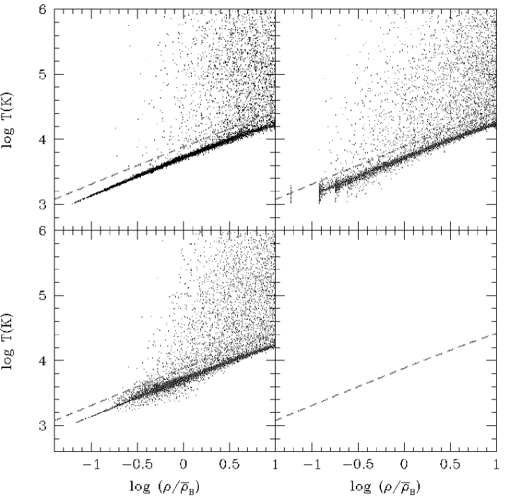
Figure 33: Density-temperature distributions at $z=2$ of runs 22-64-k using a) APMSPH , b) HYDRA without reconstruction, and c) HYDRA after reconstruction. In panel d) the solid curve shows $\log T_{\rm min}(\rho)$ for the gas (see figure 2), and its approximated power-law form as given by equation (55). The dotted line shows the equilibrium temperature of the gas (where heating balances cooling). The dashed lines in each panel are identical and the same as those plotted and defined in figure 2.

A.4 Calculation of spectra

Given the positions, velocities, densities and temperatures of all SPH particles at a given redshift, we compute spectra along a given line of sight through the box as follows. We divide the sight line into $N\sim 1000$ bins of width $\Delta$ in distance $x$ along the sight line. For a bin $i$ at position $x(i)$ we compute the density and the density weighted temperature and velocity from:

$$\rho_{X}(j) = a^{3}\,\sum_{i}X(i){\cal W}_{ij}$$ (28)

$$(\rho T)_{X}(j) = a^{3}\,\sum_{i}X(i)T(i){\cal W}_{ij}$$ (29)

$$(\rho v)_{X}(j) = a^{3}\,\sum_{i}X(i)(a\dot{x}(i)+\dot{a}(x(i)-x(j)){\cal W}_{ij}\,.$$

where $X(i)$ is the abundance of species $X$ of SPH particle $i$, assuming ionization equilibrium ($X={\mbox{${\rm H{\sc i}~{}}$}}$, $X={\mbox{${\rm He{\sc ii}~{}}$}}$; $X=1$ denotes total gas density, see Appendix A.1 for meaning of other symbols). Labelling bins according to velocity, from zero to $\dot{a}L$, a bin at velocity $v(k)$ will suffer absorption from the bin at velocity $v(j)$ by an amount $e^{-\tau(k)}$ where

$$\tau(k) = \sigma_{\alpha}{c\over V_{X}(j)}\rho_{X}(j)a\Delta$$ (31)

$$\times \exp\left(-\left[{v(k)-v(j)\over V_{X}(j)}\right]^{2}\right)/\sqrt{\pi}$$

$$V_{X}^{2}(j) = {2k_{B}T_{X}(j)/m_{X}}.$$ (32)

Here, $c$ is the light speed and $V_{X}$ is the Doppler width of the species with particles mass $m_{X}$. The Lyman-$\alpha$ cross section is $\sigma_{\alpha}=(3\pi\sigma_{T}/8)^{1/2}f\lambda_{0}$, where $\sigma_{T}=6.625\times 10^{-25}$ cm² is the Thomson cross section, $f=0.41615$ is the oscillator strength and $\lambda_{0}$ is the rest wavelength of the transition. For the hydrogen Lyman-$\alpha$ transition, we take $\lambda_{0}=1215.6{\mbox{\AA}}$ ($\sigma_{\alpha}=4.45\times 10^{-18}$ cm²), for ${\rm He{\sc ii}~{}}$, $\lambda_{0}=304.8{\mbox{\AA}}$ ($\sigma_{\alpha}=1.12\times 10^{-18}$ cm². These spectra can converted from ‘velocity’  $v$ to ‘observed’  wavelength $\lambda$ using $\lambda=\lambda_{0}\,(1+z)(1+v/c)$.

Appendix B Atomic processes and photo-ionization rates

Our simulations include all the physical processes relevant for the problem of studying primordial gas dynamics in a photo ionised intergalactic medium, as first collected by Black (1981), and whose completeness is well addressed elsewhere (see e.g. Katz et al. (1996b) and references therein). In this Appendix we briefly detail the functional form of the atomic physics coefficients used. Both APMSPH and HYDRA use the same set of coefficients, all of which are based on those collected by Cen (1992) specifically for use in cosmological hydrodynamic simulations. A few adjustments were made where improvements in accuracy or economy were found after comparison with fits used by Efstathiou (1992). Where differences occur these have also checked out satisfactorily against those quoted using updated atomic data by Abel et al. (1997), as detailed below.

We calculate the normalised radiative cooling function, ${\cal C}$ (normalised as in equation. (9) such that the rate of loss of thermal energy per unit volume, $\rho du/dt=n^{2}_{\rm H}{\cal C}$) by summing the cooling rates whose units and functional dependence on temperature are given in Table LABEL:table:cooling, such that

$${\cal C}=\sum^{11}_{i=1}c_{i}(T,\rho_{B},J(\nu,z),T_{\rm CMB})$$ (33)

The functions used to fit the $c_{i}$ are those of Cen (1992), where we have increased the collisional ionization cooling rates by a factor 2 to offset the reducing effects of the $(1+(T/10^{5}K)^{1/2})^{-1}$ factor introduced by Cen to extend the validity of existing fits to higher temperatures (this factor 2 was analogously applied to our collisional ionization rates $\Gamma_{e{\rm H{\sc i}},{\rm He{\sc i}},{\rm He{\sc ii}}}$ given below).

In order to compute cooling rates as given in Table LABEL:table:cooling we need ionic abundances for the different gas species. Normalising fractional densities to the total hydrogen density, and denoting them by their standard species nomenclature (e.g. ${\mbox{${\rm H{\sc i}~{}}$}}=n_{{\rm H{\sc i}}}/n_{\rm H}$), we may write the equations of ionization evolution as

$${d{\mbox{${\rm H{\sc i}~{}}$}}\over dt} = \alpha_{\rm H{\sc ii}}\,n_{e}{\mbox{${\rm H{\sc ii}~{}}$}}-{\mbox{${\rm H{\sc i}~{}}$}}(\Gamma_{\gamma{\rm H{\sc i}}}+\Gamma_{e{\rm H{\sc i}}}\,n_{e})$$ (34)

$${d{\mbox{${\rm He{\sc i}~{}}$}}\over dt} = \alpha_{\rm He{\sc ii}}n_{e}{\mbox{${\rm He{\sc ii}~{}}$}}-{\mbox{${\rm He{\sc i}~{}}$}}(\Gamma_{\gamma{\rm He{\sc i}}}+\Gamma_{e{\rm He{\sc i}}}n_{e})$$ (35)

$${d{\mbox{${\rm He{\sc iii}~{}}$}}\over dt} = {\mbox{${\rm He{\sc ii}~{}}$}}(\Gamma_{\gamma{\rm He{\sc ii}}}+\Gamma_{e{\rm He{\sc ii}}}n_{e})-\alpha_{\rm He{\sc iii}}{\mbox{${\rm He{\sc iii}~{}}$}}n_{e}\,$$

supplemented with the closing conditions

$${\mbox{${\rm H{\sc i}~{}}$}}+{\mbox{${\rm H{\sc ii}~{}}$}} = 1$$ (37)

$${\mbox{${\rm He{\sc i}~{}}$}}+{\mbox{${\rm He{\sc ii}~{}}$}}+{\mbox{${\rm He{\sc iii}~{}}$}} = y$$ (38)

$${\mbox{${\rm H{\sc ii}~{}}$}}+{\mbox{${\rm He{\sc ii}~{}}$}}+2{\mbox{${\rm He{\sc iii}~{}}$}} = e,$$ (39)

where $y=Y/(m_{He}/m_{H}(1-Y))$ denotes the helium abundance by number; $m_{H},m_{He}$ are the hydrogen and helium atomic mass, $n_{e}=en_{H}$ is the electron number density, and the ionization and recombination rates’ units and functional dependence on temperature are given in Tables 3, 4 & LABEL:table:photo. Assuming photo-ionization equilibrium we solve the resulting set of closed equations iteratively until the fractional change in all species densities has dropped below 0.001%.

For the recombination and collisional ionization rates’ dependence on temperature $T$, we used the functional fits listed in Table 3. Once again these are based on those of Cen (1992), but in addition to the high temperature factor correction mentioned above we introduce a factor 0.75 to reconcile the fit quoted for the ${\rm H{\sc ii}~{}}$ion recombination rate, with the data points given in Spitzer (1978). This inconsistency between Cen’s fit and Spitzer’s data has already been noted in Rauch et al. (1997, sec. 3.1) where they introduce a similar factor 0.8, and does not appear to be present for the ${\rm He{\sc iii}~{}}$ion recombination rate coefficient used.

The rate of photo-ionization of any species ion $i$, $\Gamma_{\gamma i}$, depends on the flux spectrum of ionising ultraviolet background photons, $J(\nu,z)$ (erg cm^-2 s^-1 Hz^-1 sr^-1 ), in the following way:

$$\Gamma_{\gamma i}(z) = \int^{\infty}_{\nu_{i}}\frac{J(\nu,z)\sigma_{i}(\nu)}{h\nu}\,d\nu\,,$$ (40)

where $\sigma_{i}(\nu)$ and $\nu_{i}$ are the photo-ionization cross-sections and ionising threshold frequencies respectively for each species. Similarly, excess energy in electrons ejected through photo-ionization provides a gas heating mechanism from the UV background, for which the normalised photo-heating function ${\cal H}$ (again normalised as in equation (9) such that the rate of gain in thermal energy per unit volume, $\rho du/dt=n^{2}_{\rm H}{\cal H}$) is given by,

$${\cal H}=\left({\mbox{${\rm H{\sc i}~{}}$}}\,\epsilon_{\gamma{\rm H{\sc i}}}+{\mbox{${\rm He{\sc i}~{}}$}}\,\epsilon_{\gamma{\rm He{\sc i}}}+{\mbox{${\rm He{\sc ii}~{}}$}}\,\epsilon_{\gamma{\rm He{\sc ii}}}\right)/n_{\rm H}\,.$$ (41)

Here the photo-heating coefficients used, $\epsilon_{\gamma}$, are calculated via an analogous expression to equation 40:

$$\epsilon_{\gamma i}(z)=\int^{\infty}_{\nu_{i}}\frac{J(\nu,z)\sigma_{i}(\nu)(h\nu-h\nu_{i})}{h\nu}\,d\nu\,,$$ (42)

where $h\nu_{i}$ is the ionization energy.

In this paper we assume two separate models for the UV background history of the universe. These are implemented by deducing photo-ionization and photo-heating rates using the above equations. We describe the actual fits implemented for each coefficient here.

In case of the evolving background UV spectrum computed by Haardt & Madau (1996, with deceleration parameter $q_{0}=0.5$, corresponding QSO z-evolution, and QSO spectral index equal to 1.5), we performed these integrations numerically using $\sigma_{i}(\nu)$ given by Cen (1992). Our own fits to these integrated photo-ionization and heating rates as a function of redshift, given in Table 4, are accurate at all redshifts to within 8% and also agree with fits calculated for the same spectra independently (Haardt, private communication) to within 2% (beyond $z=9$ all the rates were set to zero).

As a second more general case we assume a background of ionising photons with a power-law spectrum of the standard form:

$$J(\nu)=J_{21}\times 10^{-21}\left({\nu\over\nu_{\rm H{\sc i}}}\right)^{-\alpha}{\rm erg\,s^{-1}\,cm^{-2}\,sr^{-1}\,Hz^{-1}},$$ (43)

where the background flux is normalised by parameter $J_{21}$ at the ${\rm H{\sc i}~{}}$Lyman limit frequency $\nu_{\rm H{\sc i}}$. We can integrate equations 40 & 42 in general if we approximate the ion-photon cross-sections, $\sigma_{i}$, as having simple power-law dependencies on frequency. This is already the case for $\sigma_{\rm He{\sc i}}$, however for the hydrogenic ions ${\rm H{\sc i}~{}}$and ${\rm He{\sc ii}~{}}$we use

$$\sigma_{i}(\nu) = 6.3\times 10^{-18}{\rm cm}^{2}{f_{i}\over Z^{2}}\left(\frac{\nu_{i}}{\nu}\right)^{3}\,,$$ (44)

where $Z$ denotes the atomic number; $f_{i}\sim 1$ is a dimensionless constant. By using $f_{{\rm H{\sc i}},{\rm He{\sc ii}}}=1,1.21$ for the photo-ionization rates and $f_{{\rm H{\sc i}},{\rm He{\sc ii}}}=1.12,1.26$ for the heating rates, the resulting expressions (given in Table LABEL:table:photo) agree to 2% for a wide range of spectral index, $\alpha$, with numerical integrations using the exact $\sigma_{i}(\nu)$.

Table 2: Cooling rates (ergs cm³ s^-1). $z\equiv$ redshift, $n_{H}\equiv$ hydrogen number density and $T_{n}\equiv T/(10^{n}K)$. $T$ is in $K$.

		Collisional ionization cooling	Species
$c_{1}$	=	$2.54\times 10^{-21}T^{1/2}e^{-157809.1/T}(1+T_{5}^{1/2})^{-1}e{\mbox{${\rm H{\sc i}~{}}$}}$	${\rm H{\sc i}~{}}$
$c_{2}$	=	$1.88\times 10^{-21}T^{1/2}e^{-285335.4/T}(1+T_{5}^{1/2})^{-1}e{\mbox{${\rm He{\sc i}~{}}$}}$	${\rm He{\sc i}~{}}$
$c_{3}$	=	$9.90\times 10^{-22}T^{1/2}e^{-631515./T}(1+T_{5}^{1/2})^{-1}e{\mbox{${\rm He{\sc ii}~{}}$}}$	${\rm He{\sc ii}~{}}$
		Recombination cooling
$c_{4}$	=	$8.70\times 10^{-27}T^{1/2}T_{3}^{-0.2}(1+T_{6}^{0.7})^{-1}e{\mbox{${\rm H{\sc ii}~{}}$}}$	${\rm H{\sc ii}~{}}$
$c_{5}$	=	$1.55\times 10^{-26}T^{0.3647}e{\mbox{${\rm He{\sc ii}~{}}$}}$	${\rm He{\sc ii}~{}}$
$c_{6}$	=	$3.48\times 10^{-26}T^{1/2}T_{3}^{-0.2}(1+T_{6}^{0.7})^{-1}e{\mbox{${\rm He{\sc iii}~{}}$}}$	${\rm He{\sc iii}~{}}$
		Dielectronic recombination cooling
$c_{7}$	=	$1.24\times 10^{-13}T^{-1.5}e^{-470000./T}(1+0.3e^{-94000/T})e{\mbox{${\rm He{\sc ii}~{}}$}}$	${\rm He{\sc ii}~{}}$
		Collisional excitation cooling
$c_{8}$	=	$7.5\times 10^{-19}e^{-118348/T}(1+T_{5}^{1/2})^{-1}e{\mbox{${\rm H{\sc i}~{}}$}}$	${\rm H{\sc i}~{}}$
$c_{9}$	=	$5.54\times 10^{-17}T^{-0.397}e^{-473638/T}(1+T_{5}^{1/2})^{-1}e{\mbox{${\rm He{\sc ii}~{}}$}}$	${\rm He{\sc ii}~{}}$
		Bremsstrahlung
$c_{10}$	=	$1.42\times 10^{-27}g_{f}T^{1/2}e({\mbox{${\rm H{\sc ii}~{}}$}}+{\mbox{${\rm He{\sc ii}~{}}$}}+4{\mbox{${\rm He{\sc iii}~{}}$}})$	${\mbox{${\rm H{\sc ii}~{}}$}},{\mbox{${\rm He{\sc ii}~{}}$}},{\mbox{${\rm He{\sc iii}~{}}$}}$
$g_{f}$	=	$1.1+0.34e^{-((5.5-\log_{10}(T))^{2})/3}$
		Inverse Compton cooling
$c_{11}$	=	$5.406\times 10^{-36}\,(T-2.7(1+z))(1+z)^{4}e/n_{H}$

Table 3: Recombination and collisional ionization rates in s^-1, as a function of temperature $T$(K).

		Recombination
$\alpha_{{\rm H{\sc ii}}}$	=	$6.30\times 10^{-11}T^{-1/2}T_{3}^{-0.2}/(1+T_{6}^{0.7})$
$\alpha_{{\rm He{\sc ii}}}$	=	$1.50\times 10^{-10}T^{-0.6353}$
$\alpha_{\rm He{\sc iii}}$	=	$3.36\times 10^{-10}T^{-1/2}T_{3}^{-0.2}/(1+T_{6}^{0.7})+\alpha_{{\rm He{\sc ii}}}^{(D)}$
		Dielectronic recombination
$\alpha_{{\rm He{\sc ii}}}^{(D)}$	=	$1.9\times 10^{-3}T^{-1.5}e^{-4.7\times 10^{5}/T}(1+0.3e^{-9.4\times 10^{4}/T})$
		Collisional ionization
$\Gamma_{e{\rm H{\sc i}}}$	=	$1.17\times 10^{-10}T^{1/2}e^{-157809.1/T}\,(1+T_{5}^{1/2})^{-1}$
$\Gamma_{e{\rm He{\sc i}}}$	=	$4.76\times 10^{-11}T^{1/2}e^{-285335.4/T}\,(1+T_{5}^{1/2})^{-1}$
$\Gamma_{e{\rm He{\sc ii}}}$	=	$1.14\times 10^{-11}T^{1/2}e^{-631515/T}\,(1+T_{5}^{1/2})^{-1}$

Table 4: photo-ionization ($\Gamma_{\gamma}$ in s^-1) and photo-heating ($\epsilon_{\gamma}$ in erg s^-1) rates: Haardt & Madau spectrum. ($z\equiv$ redshift)

	Ionization rates
$\Gamma=e^{x_{1}+zx_{2}+z^{2}x_{3}}$	$x_{1}$	$x_{2}$	$x_{3}$
$\Gamma_{\gamma{\rm H{\sc i}}}$	-31.04	2.795	-0.5589
$\Gamma_{\gamma{\rm He{\sc i}}}$	-31.08	2.822	-0.5664
$\Gamma_{\gamma{\rm He{\sc ii}}}$	-34.30	1.826	-0.3899
	Photo-heating rates
$\epsilon=e^{x_{1}+zx_{2}+z^{2}x_{3}}$	$x_{1}$	$x_{2}$	$x_{3}$
$\epsilon_{{\rm H{\sc i}}}$	-56.62	2.788	-0.5594
$\epsilon_{\gamma{\rm He{\sc i}}}$	-56.06	2.800	-0.5531
$\epsilon_{\gamma{\rm He{\sc ii}}}$	-58.67	1.888	-0.3947

Table 5: photo-ionization ($\Gamma_{\gamma}$ in s^-1) and photo-heating ($\epsilon_{\gamma}$ in erg s^-1) rates: power-law spectra (Compare with equation (43) for $J_{21},\alpha$ definition).

		Ionization rates
$\Gamma_{\gamma{\rm H{\sc i}}}$	=	$1.26\times 10^{-11}J_{21}(3+\alpha)^{-1}$
$\Gamma_{\gamma{\rm He{\sc i}}}$	=	$1.48\times 10^{-11}J_{21}\,0.553^{\alpha}J_{21}\,({1.66\over\alpha+2.05}-{0.66\over\alpha+3.05})$
$\Gamma_{\gamma{\rm He{\sc ii}}}$	=	$3.34\times 10^{-12}J_{21}\,0.249^{\alpha}\,(3+\alpha)^{-1}$
		Photo-heating rates
$\epsilon_{{\rm H{\sc i}}}$	=	$2.91\times 10^{-22}J_{21}(2+\alpha)^{-1}(3+\alpha)^{-1}$
$\epsilon_{\gamma{\rm He{\sc i}}}$	=	$5.84\times 10^{-22}J_{21}\,0.553^{\alpha}\,({1.66\over\alpha+1.05}-{2.32\over\alpha+2.05}+{0.66\over\alpha+3.05})$
$\epsilon_{\gamma{\rm He{\sc ii}}}$	=	$2.92\times 10^{-22}J_{21}\,0.249^{\alpha}\,(2+\alpha)^{-1}(3+\alpha)^{-1}$

Appendix C Evaluating the IGM temperature

In this Appendix we write down the defining equations needed to solve for the temperature at given density in the high redshift universe observable through Lyman-$\alpha$ absorption where the net (heating$-$cooling) time, or ‘heating time’, $t_{\rm heat}$ is equal to the Hubble time $t_{\rm H}$,

$$t_{\rm heat}(\rho,T,J(\nu),z)=t_{{\rm H}}(z)\,.$$ (45)

We particularly show that for low densities, this relation approximates very well a power-law whose amplitude and slope are well-defined, and dependent only weakly on a few parameters, most notably the (effective) UV background spectral index (see also Hui & Gnedin 1997).

We define the Hubble time as follows for an Einstein de-Sitter universe,

$$t_{\rm H}={1\over(6\pi G\bar{\rho}(z))^{1/2}}={t^{\prime}_{\rm H}\over(1+z)^{3/2}h}\,.\\$$ (46)

The heating time (or net cooling time) defined in equation (2) may be written in general as

$$t_{\rm heat} = {3m_{\rm H}k_{B}\over 2(1-Y)^{2}\mu\bar{\rho}_{0}}{T\over\Omega_{B}\Delta_{B}h^{2}L(1+z)^{3}}$$ (47)

$$= {t^{\prime}_{{\rm heat}}T\over\Omega_{B}h^{2}\Delta_{B}L(1+z)^{3}}\,\,,$$

where we use $L={\cal H}-{\cal C}$ to denote the heating rate (erg s^-1 cm³), positive for net heating, and $\Delta_{B}=\rho_{B}/\bar{\rho}_{B}(z)$. Above and in what follows all fundamental atomic parameters are collected together into constant factors (each given a dash), so that the relative contribution from each respective process together with cosmological parameters may be preserved through the calculation. It should be noted that although these factors are denoted by the quantity they attribute to plus a dash, they will not in general have the same units as this quantity.

Using the equations as laid out in Appendix A.1 we may calculate $L$ for a given density and temperature (and UV background) and solve equation (45) in a numerical fashion straightforwardly. We can however simplify the above equation considerably by approximating the normalised cooling rates in the low-density regime.

Effectively in the low density region, $\Delta_{B}<10$, the heating rate, $L$, is dominated by ${\rm H{\sc i}~{}}$& ${\rm He{\sc ii}~{}}$photo-heating, with a small but non-negligible Compton cooling contribution. Following the notation of the previous Appendix we may write the photo-heating component of $L$, denoted $L_{\epsilon}$, simply as

$$L_{\epsilon}={\mbox{${\rm H{\sc i}~{}}$}}\frac{\epsilon_{{\rm H{\sc i}}}}{n_{\rm H}}+{\mbox{${\rm He{\sc ii}~{}}$}}\frac{\epsilon_{{\rm He{\sc ii}}}}{n_{\rm H}}\,.$$ (48)

The ${\rm H{\sc i}~{}}$${\rm He{\sc ii}~{}}$and electron fractions above are likely to be extremely highly photo-ionised and so we may write their abundances accurately as follows

$${\mbox{${\rm H{\sc i}~{}}$}}=\frac{\alpha_{{\rm H{\sc ii}}}n_{e}}{\Gamma^{\gamma}_{{\rm H{\sc i}}}}\,,\\ {\mbox{${\rm He{\sc ii}~{}}$}}=y\frac{\alpha_{{\rm He{\sc iii}}}n_{e}}{\Gamma^{\gamma}_{{\rm He{\sc ii}}}}\,,\\ e=1+2y\,,$$ (49)

where the recombination coefficients can be well approximated for temperatures $T<10^{5}$ K as (see Table 3),

$$\alpha_{{\rm H{\sc ii}}}=\alpha_{{\rm H{\sc ii}}}^{\prime}T^{-0.7}\,,\\ \alpha_{{\rm He{\sc iii}}}=\alpha_{{\rm He{\sc iii}}}^{\prime}T^{-0.7}\,.$$ (50)

Further, if we model the photo-ionization flux $J_{\nu}$ as a power law according to equation (43), then the ratios of photo-heating and photo-ionization coefficients given in Table LABEL:table:photo are

$$\frac{\epsilon_{{\rm H{\sc i}}}}{\Gamma^{\gamma}_{{\rm H{\sc i}}}}=\frac{h_{P}c}{\lambda_{{\rm H{\sc i}}}(2+\alpha)}\,,\\ \frac{\epsilon_{{\rm He{\sc ii}}}}{\Gamma^{\gamma}_{{\rm He{\sc ii}}}}=\frac{h_{P}c}{\lambda_{{\rm He{\sc ii}}}(2+\alpha)}\,,$$ (51)

where $\lambda_{{\rm H{\sc i}}}$ and $\lambda_{{\rm He{\sc ii}}}$ are the ionization wavelengths for ${\rm H{\sc i}~{}}$and ${\rm He{\sc ii}~{}}$respectively, and we denote Planck’s constant and the speed of light as $h_{P},c$. Drawing these elements together, the normalised photo-heating rate becomes

$$L_{\epsilon}=\left(\frac{\alpha_{{\rm H{\sc ii}}}^{\prime}}{\lambda_{{\rm H{\sc i}}}}+y\frac{\alpha_{{\rm He{\sc iii}}}^{\prime}}{\lambda_{{\rm He{\sc ii}}}}\right)\frac{h_{P}c(1+2y)T^{-0.7}}{2+\alpha}=\frac{L^{\prime}_{\epsilon}T^{-0.7}}{2+\alpha}\,.$$ (52)

As mentioned previously their is also a small contribution from Compton cooling, $L_{\rm cc}$, which may be written ($c_{11}$ from Table LABEL:table:cooling, $T\gg T_{\rm CMB}$)

$$L_{\rm cc}=-\frac{5.406{\times 10^{-36}}(1+2y)m_{h}}{(1-Y)\bar{\rho_{0}}}\frac{T(1+z)}{\Omega_{B}h^{2}\Delta_{B}}=\frac{L^{\prime}_{\mathrm{cc}}T(1+z)}{\Omega_{B}h^{2}\Delta_{B}}\,.$$ (53)

We are now in a position to solve for the temperature at a given density where $t_{\rm heat}=t_{H}$. Substituting for each using equations 46, 47, 52 and 53

$$\frac{t^{\prime}_{\rm heat}T}{\Omega_{B}h^{2}\Delta_{B}}=\left(\frac{L^{\prime}_{\epsilon}T^{-0.7}}{2+\alpha}+\frac{L^{\prime}_{\rm cc}T(1+z)}{\Omega_{B}h^{2}\Delta_{B}}\right){t^{\prime}_{\rm H}(1+z)^{3/2}\over h}\,,$$ (54)

which by multiplying through by $\Omega_{B}h^{2}\Delta_{B}/T$ and juggling yields the general solution for $T$ at given $\Delta_{B}$,

$$T = T_{0}\Delta_{B}^{\frac{1}{1.7}}$$ (55)

$$T_{0} = \left[\left(\frac{\Omega_{B}L^{\prime}_{\epsilon}t^{\prime}_{\rm H}}{t^{\prime}_{\rm heat}h}\frac{(1+z)^{3/2}}{2+\alpha}\right)\bigg{/}\left(1-\frac{L^{\prime}_{\rm cc}t^{\prime}_{\rm H}(1+z)^{5/2}}{t^{\prime}_{\rm heat}h}\right)\right]^{{1\over 1.7}}\,.$$

The second factor in brackets encloses the contribution of Compton cooling only. This is found always to be small for intermediate redshifts. Putting in values for physical constants, using a cosmological helium fraction, $Y=0.24$, and $\mu=(1+4y)/(1+y+e)=0.588$ in the low density limit, we get

$$t^{\prime}_{\rm H{\sc i}} = 2.06{\times 10^{17}}\;{\rm s}$$ (57)

$$t^{\prime}_{\rm heat} = 5.41{\times 10^{-11}}\;{\rm erg}\;{\rm cm}^{3}\;{\rm K}^{-1}$$ (58)

$$L^{\prime}_{\epsilon} = 1.70{\times 10^{-20}}\;{\rm erg}\;{\rm s}^{-1}\;{\rm cm}^{3}\;{\rm K}^{0.7}$$ (59)

$$L^{\prime}_{\rm cc} = -7.31{\times 10^{-30}}\;{\rm erg}\;{\rm s}^{-1}\;{\rm cm}^{3}\;{\rm K}^{-1}\,,$$ (60)

where we have used the following atomic numbers for $L^{\prime}_{\epsilon}$:

$$\lambda_{{\rm H{\sc i}}} = 911.75{\mbox{\AA}}$$ (61)

$$\lambda_{{\rm He{\sc ii}}} = 227.67{\mbox{\AA}}$$ (62)

$$\alpha_{{\rm H{\sc ii}}}^{\prime} = 2.51{\times 10^{-10}}\;{\rm K}^{0.7}\;{\rm s}^{-1}$$ (63)

$$\alpha_{{\rm He{\sc iii}}}^{\prime} = 1.34{\times 10^{-9}}\;{\rm K}^{0.7}\;{\rm s}^{-1}\,,$$ (64)

which may be collected together into equation (C) above to find

$$T_{0}=\frac{3.92{\times 10^{4}}(1+z)^{3\over 3.4}(\Omega_{B}h/(2+\alpha))^{1\over 1.7}}{\left(1+{1\over h}\left(\frac{1+z}{1+9.52}\right)^{5/2}\right)^{\frac{1}{1.7}}}\;{\rm K}\,,$$ (65)

where the main dependencies for $T_{0}$ are given in the numerator, and the denominator has the correction due to Compton cooling only.

References

- [Abel et al. 1997] Abel, T., Anninos, P., Zhang, Y., Norman, M.L., 1997, New Astronomy, vol. 2, no. 3, p. 181-207.
- [Bardeen et al. 1986] Bardeen J.M., Bond J.R., Kaiser N., Szalay A.S., 1986, ApJ, 304,15
- [Black 1981] Black, J. H., 1981, MNRAS, 197, 553
- [Bond & Wadsley 1997] Bond, J.R, Wadsley, J., 1997, To appear in ”Computational Astrophysics”, Proc. 12th Kingston Conference, Halifax, Oct. 1996, ed. D. Clarke & M. West (PASP), astro-ph/9703125
- [] Burles, S., Tytler, D., 1997, to appear in ISSI workshop Primordial Nuclei and their Galactic Evolution, Edts. N. Prantzos, M. Tosi, & R. von Steiger (astro-ph/9712265)
- [Carswell et al. 1987] Carswell, R.F., Webb, J.K., Baldwin, J.A., Atwood, B., 1987, ApJ, 319, 709
- [Cen 1992] Cen, R., 1992, ApJS, 78, 341
- [Cen et al. 1994] Cen, R., Miralda’Escudé, J., Ostriker, J.P., Rauch, M., 1994, ApJL, 437, L83
- [] Colberg, J.M., White, S.D.M., Jenkins, A., Pearce, F.R., Frenk, C.S., Thomas, P.A., Hutchings, R., Couchman, H.M.P., Peacock, J.A., Efstathiou, G.P., Nelson A.H., (The Virgo Consortium), 1997, Proceedings of Ringberg Workshop on Large Scale Structure (astro-ph/9702086)
- [Couchman 1991] Couchman, H.M.P., 1991, ApJL, 368, L23
- [Couchman, Thomas & Pearce 1995] Couchman, H.M.P., Thomas, P.A., Pearce, F.P., 1995, ApJ, 452, 797
- [Croft et al. 1997] Croft, R.A.C., Weinberg, D.H., Katz, N., Hernquist, L., 1997, ApJ 488, 532
- [Croft et al. 1998] Croft, R.A.C., Weinberg, D.H., Katz, N., Hernquist, L., 1998, ApJ, 495, 44
- [Dave] Davé, R., Hernquist, L., Weinberg, D.H., Katz, N., 1997, ApJ, 477, 21
- [] Davidsen, A.F., Kriss, G.A., Zheng, W., 1996, Nature, 380, 47
- [Efstathiou 1992] Efstathiou, G., 1992, MNRAS , 256, 43
- [Efstathiou et al. 1985] Efstathiou, G., Davis, M., Frenk, C.S., White, S.D.M., 1985, ApJS, 57, 241
- [] Eke, V.R., Cole, S., Frenk, C.S., 1996, MNRAS, 282, 263
- [Evrard] Evrard, A.E., 1988, MNRAS, 911
- [] Fardal, M.A., Giroux, M.L., Shull, J.M., 1998, astro-ph/9802246
- [Gingold & Monaghan 1977] Gingold, R.A., Monaghan, J.J., 1977, MNRAS, 181, 375
- [Giroux & Shapiro 1996] Giroux, M.L., Shapiro P.R., 1996, ApJS, 102, 191
- [GP65] Gunn, J.E., Peterson, B.A., 1965, ApJ, 142, 1633
- [Haardt & Madau 1996] Haardt, F., Madua, P., 1996, ApJ, 461, 20
- [Haehnelt & Steinmetz 1998] Haehnelt, M.G., Steinmetz, M., 1998, MNRAS, in press (astro-ph/9706296)
- [Hernquist & Katz 1989] Hernquist, L., Katz, N., 1989, ApJS, 70,419
- [Hernquist et al. 96] Hernquist, L., Katz, N., Weinberg, D.H, Miralda-Escudé, J., 1996, ApJL, 457, 51
- [Hockney & Eastwood 1988] Hockney, R.W., Eastwood, J.W., 1988, Computer Simulations Using particles (Bristol: IOP Publishing Ltd.)
- [Hu et al. (1995)] Hu, E.M., Kim, T., Cowie, L.L., Songaila, A., Rauch, M., 1995, AJ, 110, 1526 (HKCSR)
- [] Hui, L., Gnedin, N., 1997, MNRAS, 292, 27
- [] Jakobsen, P., 1997, Nature, 387, 348
- [Jenkins et al. 1997] Jenkins, A., Frenk, C.S., Thomas, P.A., Colberg, J.M., White, S.D.M., Couchman, H.M.P., Peacock, J.A., Efstathiou, G.P., Nelson, A.H., (The Virgo Consortium), 1998, ApJ in press, astro-ph/9709010
- [] Katz, N., Weinberg, D.H., Hernquist, L., Miralda-Escudé, J.M., 1996a, 457, L57
- [Katz, Weinberg & Hernquist 1996b] Katz, N., Weinberg, D.H., Hernquist L., 1996b, ApJS, 105, 19
- [Kim et al. 1997] Kim, T., Hu, E.M., Cowie, L.L., Songaila, A., 1997, AJ, 114, 1 (KHCS)
- [Leonard 1988] Leonard, A.P.B., 1998, PhD Thesis, Oxford University
- [] Lu, L., Sargent ,W.L.W., Womble D.S., Takada-Hidai M., 1996, ApJ, 472, 509
- [Lucy 1970] Lucy, L.B., 1977, AJ, 82, 1023
- [Lynds 1971] Lynds, C.R., 1971, ApJ, 164, L73
- [] Miralda-Escudé, J.M., 1993, MNRAS, 262, 273
- [Miralda-Escudé & Rees 1994] Miralda-Escudé, J., Rees, M.J., 1994, MNRAS, 266, 343
- [] Miralda-Escudé, J., Cen, R., Ostriker, J.P., Rauch, M., 1996, ApJ, 471, 582
- [Monaghan 1992] Monaghan, J.J., 1992, ARA&A 30, 543
- [Navarro, Frenk & White 1996] Navarro, J.F., Frenk, C.S., White, S.D.M., 1996, ApJ, 462, 563
- [Pearce et al. 1998a] Pearce, F.R., Jenkins, A., Frenk, C.S., Thomas, P.A., Colberg, J.M., White, S.D.M., Couchman, H.M.P., Peacock, J.A., Efstathiou, G.P., Nelson, A.H., (The Virgo Consortium), 1998, in preparation
- [Petitj96] Petitjean, P., Webb, J.K., Rauch, M., Carswell, R.F., Lanzetta, K., 1993, MNRAS, 262, 499 (PWRCL)
- [Peebles 1980] Peebles, P.J.E., 1980, The Large-Scale Structure of the Universe (Princeton: Princeton Univ. Press)
- [Rauch et al. 1997] Rauch, M., Miralda-Escudé, J., Sargent, W.L.W., Barlow, T.A., Weinberg, D.H., Hernquist, L., Katz, N., Cen, R., Ostriker, J.P., 1997, ApJ, 489, 7
- [] Reimers, D., Kohler, S., Wisotzski, L., Groote, D., Rodriguez-Pascual, P, Wamsteker, W., 1997, A&A, 327, 890
- [Spitzer 1978] Spitzer, L., Jr., 1978. Physical Processes in the Interstellar Medium, (New York: Wiley)
- [] Theuns, T., Leonard, A.P.B., Efstathiou, G., 1998, to be published by MNRAS (astro-ph/9803245)
- [Wadsley & Bond 1996] Wadsley, J., Bond, J.R, 1996, to appear in ”Computational Astrophysics”, Proc. 12th Kingston Conference, Halifax, Oct. 1996, ed. D. Clarke & M. West (PASP) (astro-ph/9612148)
- [Walker] Walker, T.P., Steigman, G., Schramm, D.N., Olive, K.A., Kang, H.S., 1991, ApJ, 376, 51
- [Webb 1995] Webb, J.K., 1987, PhD Thesis, University of Cambridge
- [] Williger, G.M., Baldwin, J.A., Carswell, R.F., Cooke, A.J., Hazard, C., 1994, ApJ, 428, 574
- [Zel’dovich 1970] Zel’dovich, Ya. B., 1970, A&A, 5, 84
- [Zhang, Anninos & Norman, 1997] Zhang, Y., Anninos, P., Norman, M.L., 1995, ApJL, 453, L57
- [Zhang et al. 1995b] Zhang, Y., Anninos, P., Norman, M.L., 1997, ApJ, 485, 496
- [] Zhang, Y., Meiksin, A., Anninos, P., Norman, M., 1998, ApJ, 495, 63
- [] Zheng, W., Kriss, G.A., Telfer, R.C., Grimes, J.P., Davidsen, A.F., 1997, ApJ, 475, 469