Regularity in the distribution of superclusters?

Abstract

We use a measure of clustering derived from the nearest neighbour distribution and the void probability function to distinguish between regular and clustered structures. This measure offers a succinct way to incorporate additional information beyond the two–point correlation function. Application to a supercluster catalogue by ? reveals no clustering in the distribution of superclusters. However, we show that this supercluster catalogue is severely affected by construction effects. Taking these biases into account we still find some indications for regularity on the largest scales, but the significance is only at the one–$\sigma$ level.

1 Introduction

In a recent paper ? report a peak in the 3D–power spectrum of a catalogue of clusters on scales of 120$h^{-1}$Mpc. ? observed periodicity on approximately the same scales in an analysis of 1D–data from a pencil–beam redshift survey. As is well known from the theory of fluids, the regular distribution (e.g.  of molecules in a hard–core fluid) reveals itself in an oscillating two–point correlation function and a peak in the structure function respectively (see e.g. ?). In accordance with this an oscillating two–point correlation function $\xi_{2}(r)$ or at least a first peak was reported on approximately the same scale (?, ?, ?, and ?).

In this paper we analyze the supercluster catalogue of ? which was constructed from an earlier version of the cluster catalogue by ? using a friend–of–friends procedure. With methods based on the nearest neighbour distribution and the spherical contact distribution we can show that this supercluster catalogue is regular with 95% significance. However, taking into account the selection and construction effects, the high significance vanishes and we only find some indication for a regular distribution on large scales, showing that this supercluster catalogue is seriously affected by the construction method with a friend–of–friends procedure.

This paper is organized as follows. In Sect. 2 we discuss our methods. Through some examples, we illustrate the properties of the $J$-function and show that it offers a concise way to incorporate information about correlations of arbitrary order. The analysis of the supercluster distribution and of a set of mock supercluster catalogues is presented in Sect. 3. We summarize our results in Sect. 4.

2 Methods

To analyze the set of points ${\cal X}=\{{\mathbf{x}}_{i}\}_{i=1}^{N}$, ${\mathbf{x}}_{i}\in{\mathbb{R}}^{3}$ given by the redshift coordinates of the superclusters we use the spherical contact distribution $F(r)$, i.e. the distribution function of the distances $r$ between an arbitrary point and the nearest object in ${\cal X}$. $F(r)$ is equal to the expected fraction of volume occupied by points which are not farther away than $r$ from the objects in ${\cal X}$. Therefore, $F(r)$ is equal to the volume density of the first Minkowski functional as introduced into cosmology by ?. As another tool we use the nearest neighbour distribution $G(r)$, that is defined as the distribution function of distances $r$ of an object in ${\cal X}$ to the nearest other object in ${\cal X}$. For a Poisson distribution the probability to find a point only depends on the mean number density $\overline{\rho}$, leading to the well–known result

$$G_{\rm P}(r)=1-\exp\left(-\overline{\rho}\frac{4\pi}{3}r^{3}\right)=F_{\rm P}(r).$$ (1)

Recently, ? suggested to use the ratio

$$J(r)=\frac{1-G(r)}{1-F(r)}$$ (2)

as a probe for clustering of a point distribution. For a Poisson distribution $J(r)=1$ follows directly from Eq. (1). As shown by ?, a clustered point distribution implies $J(r)\leq 1$, whereas regular structures are indicated by $J(r)\geq 1$. Typical clustered structures are produced by Neyman–Scott processes Neyman & Scott (1958) which have been used to model the distribution of galaxies. Regular structures are seen in a periodic, or a crystalline arrangement of points. In a statistical sense, and opposed to clustering, regular (“ordered”) structures are also seen in liquids. Qualitatively one may explain the behaviour of $J(r)$ as follows:

• In a clustered distribution of points $G(r)$ increases faster than for a random distribution of points, since the nearest neighbour is typically in the close surroundings. $F(r)$ increases more slowly than for a random distribution, since an arbitrary point is typically inbetween the clusters. These two effects give rise to $J(r)\leq 1$.

• On the other hand, in a regular distribution of points, $G(r)$ increases more slowly than for a random distribution of points, since the nearest neighbour is typically at a finite characteristic distance (e.g. in the case of a crystal). $F(r)$ increases faster, since the typical distance from a random point to a point on a regular structure is smaller. These two effects cause $J(r)$ to be greater than unity.

• $J(r)=1$ indicates the borderline between clustered and regular structures.

2.1 Gaussian approximation

Figure 1: Above we see the two–point correlation function $\xi_{2}(r)$ of an anticorrelated point distribution (dashed), a correlated point distribution (dotted), and of a process mimicking the cluster distribution (solid); $r$ in arbirary units. Below the corresponding $J(r)$ with $\overline{\rho}=1$ in the Gaussian approximation are depicted.

For a stationary point distribution $1-F(r)$ is equal to the probability that no galaxy is inside a sphere ${\cal B}_{r}$ with radius $r$:

$$F(r)=1-\rho_{0}({\cal B}_{r}),$$ (3)

with $\rho_{0}({\cal B}_{r})$ being the void probability function White (1979). Similarly, $1-G(r)$ is equal to the probability that there is an object at ${\mathbf{x}}\in{\cal X}$ and that there is no other object inside the sphere ${\cal B}_{r}({\mathbf{x}})$ centered on ${\mathbf{x}}$:

$$G(r)=1-\frac{\rho_{1}({\mathbf{x}}\leavevmode\nobreak\ |\leavevmode\nobreak\ {\cal B}_{r}({\mathbf{x}}))}{\overline{\rho}}\rho_{0}({\cal B}_{r}({\mathbf{x}})).$$ (4)

$\rho_{1}({\mathbf{x}}\leavevmode\nobreak\ |\leavevmode\nobreak\ {\cal B}_{r}({\mathbf{x}}))$ is the density that we observe a point at ${\mathbf{x}}$ under the condition that ${\cal B}_{r}({\mathbf{x}})$ is empty. Therefore we obtain Sharp (1981):

$$J(r)=\frac{\rho_{1}({\mathbf{x}}\leavevmode\nobreak\ |\leavevmode\nobreak\ {\cal B}_{r}({\mathbf{x}}))}{\overline{\rho}}.$$ (5)

Following ? we can express the conditional density $\rho_{1}$ in terms of the $n$–point correlation functions, the normed cumulants, $\xi_{n}$ (see also ?):

$$\rho_{1}({\mathbf{x}}\leavevmode\nobreak\ |\leavevmode\nobreak\ {\cal B}_{r}({\mathbf{x}}))=\overline{\rho}-\sum_{n=1}^{\infty}\frac{(-\overline{\rho})^{n+1}}{n!}\times$$ (6)

$$\times\int_{{\cal B}_{r}({\mathbf{x}})}{\rm d}^{3}x_{1}\dots\int_{{\cal B}_{r}({\mathbf{x}})}{\rm d}^{3}x_{n}\ \xi_{n+1}({\mathbf{x}},{\mathbf{x}}_{1},\ldots,{\mathbf{x}}_{n}).$$

A Gaussian approximation, i.e. $\xi_{n}=0$ for $n>2$, yields

$$J(r)\approx 1-\overline{\rho}\ 2\pi\ \int_{0}^{r}{\rm d}s\ s^{2}\xi_{2}(s).$$ (7)

In Fig. 1 we show several two–point correlation functions $\xi_{2}(r)$, satisfying the normalization condition $\int_{0}^{\infty}{\rm d}s\ s^{2}\xi_{2}(s)=0$, and the corresponding $J(r)$ in the Gaussian approximation. From the third example (solid lines in Fig. 1) we see that a point distribution which is correlated (clustered) on small scales may show anticorrelation on large scales, such that $J(r)<1$ for small and $J(r)>1$ for large $r$. Two simple examples of a correlated distribution with $\xi_{2}(r)>0$, and of an anticorrelated distribution with $\xi_{2}(r)<0$ clearly show the expected $J(r)<1$ and $J(r)>1$ respectively.

2.2 Beyond the Gaussian approximation

According to Eqs. (5) and (6) $J(r)$ depends on correlations of arbitrary order. Therefore, a Gaussian approximation to $J(r)$ may be misleading. We illustrate this with two different point distributions: a Poisson (i.e.  random) distribution of points, and points given by the model of ?. Both point distributions exhibit the same two–point characteristics, but the example of ? is regular by construction. To generate a realization of the point distributions by ? we divide the unit square into $20\times 20$ cells and randomly place 0, 1, or 10 points into each cell, with a probability of $1/10$, $8/9$, and $1/90$ respectively. In Fig. 2 we display these point distributions with 388 points in a square. By visual inspection the set of points given by ? shows a regular structure. Larger voids are only seen in the Poisson distribution. We obtain $J(r)\geq 1$ for the regular point set, clearly distinguishable from the $J(r)=1$ for the Poisson distributed points (Fig. 3). Both have the same two point correlation function $\xi_{2}(r)=0$ by construction. No scale can be deduced from the two–point correlation function $\xi_{2}(r)$ as seen in Fig. 3. Since the number density and $\xi_{2}(r)$ are equal in both point sets, the difference in $J(r)$ results from high–order correlations only. $J(r)$ and its variance diverge near the intrinsic scale $r=1/20$ of this specific regular point distribution, since $F(r)$ approaches unity.

If we estimate $F(r)$ from one realization of a point process, $F(r)$ becomes unity when $r$ becomes larger than the radius of the biggest empty sphere which fits inside the sample. Similarly, we get $G(r)=1$ for $r$ larger than the largest distance between neighbouring objects. Therefore the estimate of the $J$–function from a single point set becomes undetermined beyond these radii. Since $J(r)$ is a global measure we are still able to detect regular structures, as global features of a point pattern, from the $J(r)\geq 1$ for radii $r$ below the intrinsic scale, here $1/20$.

As discussed in ?, $J(r)=1$ does not necessarily imply Poisson distributed points. The morphological measure $J(r)$ was used by ? to investigate large scale fluctuations in the galaxy distribution and earlier by ? to test a hierarchical model for galaxy clustering.

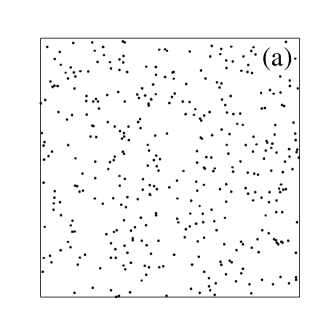
Figure 2: In plot (a) randomly distributed points and in plot (b) points from realization of the regular example by ? are displayed.

Figure 3: The plots show the two–point correlation function $\xi_{2}(r)$ on top, and $J(r)$ at the bottom for the random points (dark shaded) and for the regular example by ? (light shaded). The areas correspond to the 1$\sigma$–error estimated from fifty realizations. The dashed lines display the $J(r)$ for the point distributions shown in Fig. 2; $r$ is in units of the side length of the square.

Since all real astronomical catalogues are spatially limited we have to use edge–corrected estimators as detailed in ?. The rationale behind these estimators is to use only the points whose possible nearest neighbours are contained in the sample window. With these estimators we neither make any assumptions about the exterior of our sample, nor do we use weighting schemes. However, our analysis of the supercluster sample is restricted to a radial distance of at most 60–70$h^{-1}$Mpc.

3 Results

3.1 The supercluster sample

We use the supercluster sample compiled by ? with 220 superclusters out to $z=0.12$. The sample was generated with a friend–of–friends algorithm using a linking length of 24$h^{-1}$Mpc  from an earlier version of the cluster sample by ? and includes all superclusters of at least two member clusters. A detailed discussion of the sample is given in ?. We limit our analysis to a region within galactic latitude $|b|>20^{\circ}$ and a maximum radial distance of 330 $h^{-1}$Mpc. As directly suggested by the sample geometry we perform our analysis separately for the northern and southern parts (in galactic coordinates). 95 superclusters enter into the northern part (mainly Abell sample) and 116 superclusters into the southern part (mainly ACO sample). The selection effects are modeled with an independent radial and angular selection function (see ?).

3.2 Regular structures?

Figure 4: $J(r)$ for the northern part (dashed), the southern part (solid), and a Poisson sample (shaded area) are displayed. The curves are smoothed with a triangular kernel with a total width of 3$h^{-1}$Mpc.

In Fig. 4 the values of $J(r)$ for the supercluster distribution are plotted together with the average and $1\sigma$–error of 99 realizations of a (pure) Poisson distribution with the same sample size and geometry. A $J(r)$ larger than unity, as expected for a regular distribution of the points (see Sect. 2), is clearly seen. $J(r)$ for both parts is above one, lying outside the $1\sigma$–range of the Poisson distribution on scales from $15{h^{-1}{\rm Mpc}}$ to $50{h^{-1}{\rm Mpc}}$. The kink in $J(r)$ at $r=45{h^{-1}{\rm Mpc}}$ in the southern part and at 55$h^{-1}$Mpc in the northern part indicates the typical scale on which the nearest supercluster is situated. This agrees with the median distance to the nearest poor supercluster of $45{h^{-1}{\rm Mpc}}$ as estimated by ?. As discussed in Sect. 2 $J(r)$ becomes unreliable on scales beyond $60{h^{-1}{\rm Mpc}}$ (see also Fig. 4). With a (nonparametric) Monte–Carlo test, as described by ?, we conclude with 95% confidence that the superclusters given by ? are not compatible with Poisson distributed points with the same number density. We will see that this is not decisive, since up to now we did not include selection and construction effects.

To test the influence of the selection effects and the construction process we generate 99 “mock supercluster catalogues”. We start with Poisson distributed points within a sphere of 370$h^{-1}$Mpc incorporating the radial and angular selection effects of the galaxy cluster catalogue given by ?; then we apply a friend–of–friends procedure with linking length of 24$h^{-1}$Mpc to identify the mock “superclusters”. As seen in Fig. 5, using a friend–of–friends algorithm, we generate an empty sphere with radius of at least 24$h^{-1}$Mpc around each supercluster center, introducing an artificial anticorrelation, leading to $J(r)>1$. Therefore, the regularity seen in the northern part of the supercluster sample up to scales of 60$h^{-1}$Mpc  is at least partly an artifact of the construction. Still the southern part shows a $J(r)$ above the mean $J(r)$ of the mock superclusters, mostly outside the $1\sigma$–range, but a definite statement with a significance of 95% (roughly $2\sigma$) is no longer possible.

Figure 5: The lower solid line is the result for the northern part, the upper solid line the result for the southern part and the dashed line the result for the whole sample. The shaded area marks the $1\sigma$–range estimated from 99 mock supercluster realizations. The inset plot shows the difference $\Delta$ between the mean values of $J(r)$ for the pure Poisson process and the mock superclusters samples. All curves are smoothed with a triangular kernel with a total width of 3$h^{-1}$Mpc.

4 Discussion and Conclusion

We have shown that the statistical properties of the supercluster distribution as given by ? are seriously affected by the construction with a friend–of–friends procedure. This is not astonishing since the linking length of 24$h^{-1}$Mpc  is already one fifth of the claimed regularity scale of 120$h^{-1}$Mpc. The distinction between regular and clustered point patterns with the $J$–function is unambiguous for a homogeneous and isotropic point distribution. In such a case the borderline is given by $J(r)=1$. Our procedure for generating mock supercluster samples, where we start with a Poisson sample, include the selection effects, and redo the supercluster identification with a friend–of–friends algorithm in the same way as for the real cluster sample, results in a $J(r)\neq 1$ even though we started from a Poisson distribution. Although it is plausible, that such mock–supercluster samples describe the borderline between clustered and regular structures, there is no proof of this assertion. The apparent regularity in the northern part of the sample can be explained as a result of these construction effects, whereas the southern part still shows a trend towards regular structures outside the $1\sigma$–range.

The results for the oscillating two–point correlation function of galaxy clusters and, correspondingly the peak in the power spectrum were obtained with estimators using weighting schemes and boundary corrections, which rely heavily on the assumption of homogeneity. Up to now there is no reliable way to prove this from the three–dimensional distribution of galaxies and clusters. There are some hints that the universe reaches homogeneity on scales above several hundreds of $h^{-1}$Mpc  (see the discussions by ? versus ?). We adopted a conservative point of view and used estimators which do not make any assumptions about the distribution of superclusters outside the sample window. In Sect. 2 we showed that the $J$–function can be estimated from one point set only for scales smaller than the radius of the largest void. Therefore, we do not reach the claimed regularity scale at 120$h^{-1}$Mpc. Still, the measure $J(r)$ gives us information about global properties of the supercluster distribution, in our case a tendency towards regular structures.

We analyzed the distribution of clusters of the more recent redshift compilation by ? with the $J$–function. We found the expected clumping of galaxy clusters, as indicated by $J(r)\leq 1$. Qualitatively, the $J(r)\leq 1$ may be explained with a $\xi_{2}(r)>0$ and the Gaussian approximation in Eq. (7). This clumping out to scales of 40$h^{-1}$Mpc is confined mainly to the interior of the superclusters. Isolated ”field” clusters were not included in the supercluster sample but may contribute to the correlation seen up to scales of 50$h^{-1}$Mpcin the cluster samples. One hierarchical level higher, the supercluster centers themselves show a tendency towards regular structures. Again this can be explained qualitatively with the Gaussian approximation (see Fig. 1). A theoretical example illustrating such a hierarchical property is given by Neyman–Scott processes Neyman & Scott (1958): In such a process the overall distribution of points shows correlation (i.e. $\xi(r)>0$ for small $r$), but the cluster centers of these points are distributed randomly by construction.

Unlike the two–point correlation function the $J$–function incorporates information stemming from high order correlations. Our example in Fig. 3 illustrates, that a regular structure detected unambigously with the $J$–function may not be visible in an analysis with the two–point correlation function $\xi_{2}(r)$ alone.

Another problem is the fluctuations between the northern and southern parts of the sample. This may be attributed to the different selection effects entering the Abell and ACO parts of the sample, probably due to the different sensitivity of the photo plates used. However, in the case of the IRAS 1.2 Jy galaxy catalogue such fluctuations were shown to be real on scales of 200$h^{-1}$Mpc Kerscher et al. (1997). Also, ? find from the ESP survey, that at least in the southern hemisphere the local density is below the mean sample density out to 140$h^{-1}$Mpc. If we assume that the fluctuations decrease on scales above 200$h^{-1}$Mpc, the finding of regular structures on such large scales is a great challenge to the standard scenarios of structure formation by gravitational instability, starting from Gaussian initial density fluctuations. Implications of these regular structures for the standard scenarii of structure formation are discussed in ? and ?.

References

- Andernach & Tago (1998) Andernach H., Tago E.: 1998, In: Proc. Large Scale Structure: Tracks and Traces, Potsdam, Germany (Singapore), Müller V., Gottlöber S., Mücket J. P., Wambsgans J. (eds.), World Scientific, in press, astro-ph/9710265
- Baddeley & Silverman (1984) Baddeley A. J., Silverman B. W., 1984, Biometrics 40, 1089
- Bedford & van den Berg (1997) Bedford T., van den Berg J., 1997, Adv. Appl. Prob. 29, 19
- Besag & Diggle (1977) Besag, J., Diggle, P. J., 1977, Appl. Statist. 26, 327
- Broadhurst et al. (1990) Broadhurst T. J., Ellis R. S., Koo D. C., Szalay A. S., 1990, Nature 343, 726
- Einasto et al. (1997a) Einasto J., Einasto M., Frisch P. et al., 1997a, MNRAS 289, 801
- Einasto et al. (1997b) Einasto J., Einasto M., Frisch P. et al., 1997b, MNRAS 289, 813
- Einasto et al. (1997c) Einasto J., Einasto M., Gottlöber S. et al., 1997c, Nature 385, 139
- Einasto et al. (1997d) Einasto M., Tago E., Jaaniste J. et al., 1997d, A&AS 123, 119
- Fetisova et al. (1993) Fetisova T. S., Yu. Kuznetsov D., Lipovetskii V. A. et al., 1993, Astron. Lett. 19(3), 198
- Guzzo (1997) Guzzo L., 1997, New Astronomy 2(6), 517
- Hansen & McDonnald (1986) Hansen J. P., McDonnald I. R., 1986, Theory of simple liquids, Academic Press, New York and London
- Kerscher et al. (1997) Kerscher M., Schmalzing J., Buchert T., Wagner H. 1997, A&A in press, astro-ph/9704028
- Kopylov et al. (1988) Kopylov A. I., Yu. Kuznetsov D., Fetisova T. S., Shvartsman V. F.: 1988, In: Large Scale Structure of the Universe, Audouze J. A. et al. (ed.), IAU, pp. 129
- Mecke et al. (1994) Mecke K. R., Buchert T., Wagner H., 1994, A&A 288, 697
- Mo et al. (1992) Mo H. J., Deng Z. G., Xia X. Y. et al., 1992, A&A 257, 1
- Neyman & Scott (1958) Neyman J., Scott E. L., 1958, J. R. Stat. Soc. 20, 1
- Sharp (1981) Sharp N., 1981, MNRAS 195, 857
- Stratonovich (1963) Stratonovich R. L., 1963, Topics in the theory of random noise Vol. 1, Gordon and Breach, New York
- Sylos Labini et al. (1998) Sylos Labini F., Montuori M., Pietronero L., 1998, Physics Rep. 293, 61
- Szalay (1997) Szalay A. S.: 1997, In: Proc. of the 18th Texas Symposium on Relativistic Astrophysics (New York), Olinto, A. (ed.), AIP
- van Lieshout & Baddeley (1996) van Lieshout M. N. M., Baddeley A. J., 1996, Statist. Neerlandica 50, 344
- White (1979) White S. D. M., 1979, MNRAS 186, 145
- Zucca et al. (1997) Zucca E., Zamorani G., Vettolani G. et al., 1997, A&A 326, 477