Keck Spectroscopy of Candidate Proto–globular Clusters in NGC 1275¹

Abstract

Keck spectroscopy of 5 proto–globular cluster candidates in NGC 1275 has been combined with HST WFPC2 photometry to explore the nature and origin of these objects and discriminate between merger and cooling flow scenarios for globular cluster formation.

The objects we have studied are not HII regions, but rather star clusters, yet their integrated spectral properties do not resemble young or intermediate age Magellanic Cloud clusters or Milky Way open clusters. The clusters’ Balmer absorption appears to be too strong to be consistent with any of the standard Bruzual and Charlot evolutionary models at any metallicity. If the Bruzual and Charlot models are adopted, an IMF which is skewed to high masses provides a better fit to the proto–globular cluster candidates  data. A truncated IMF with a mass range of $\rm 2\!-\!3\,M_{\odot}\,\,$reproduces the observed Balmer equivalent widths and colors at $\sim\,$450 Myr.

Formation in a continuous cooling flow appears to be ruled out since the age of the clusters is much larger than the cooling time, the spatial scale of the clusters is much smaller than the cooling flow radius, and the deduced star formation rate in the cooling flow favors a steep rather than a flat IMF. A merger would have to produce clusters only in the central few kpc, presumably from gas in the merging galaxies which was channeled rapidly to the center. Widespread shocks in merging galaxies cannot have produced these clusters.

If these objects are confirmed to have a relatively flat, or truncated, IMF it is unclear whether or not they will evolve into objects we would regard as bona fide globular clusters.

1 Introduction

The discovery by Holtzman et al. (1992) of proto–globular cluster candidates in NGC 1275, the peculiar cD galaxy at the center of the Perseus cluster, was regarded by many as an important piece of evidence in favor of the merger model for elliptical galaxy formation (Schweizer 1987, Ashman & Zepf 1992). The Ashman & Zepf model implies that globular clusters are formed with high efficiency during a major merger of two gas–rich spiral galaxies. It has also been suggested (e.g. Fabian et al. 1984) that globular clusters can form efficiently in cooling flows. NGC 1275 has one of the largest known cooling flows (Fabian et al. 1981, Allen & Fabian 1997) and it has a Seyfert–type nucleus with strong H$\alpha$ emission, as well as a large molecular and neutral hydrogen content. A number of features including its irregular shape may be indicative of a merger history (e.g. Zepf et al. 1995).

Minkowski (1957) discovered the existence of two velocity systems in the galaxy spectrum. The low–velocity (LV) system, comprising filaments of ionized gas whose radial velocity is similar to that of the main body of NGC 1275 (i.e. 5264$\pm$11$\rm\,km\,s^{-1}$, Strauss et al. 1992), is generally thought to be a product of the cooling flow. Lazareff et al. (1989) detected significant amounts ($\sim\,$6 x 10⁹ M_⊙) of CO associated with the H$\alpha$ filaments, perhaps revealing the source of raw materials (molecular gas) from which stars/clusters might form. The association of the molecular gas with the ionized filaments was inferred from the CO and H$\alpha$ spectral line parameters (central velocity, line width and integrated intensity) which displayed similar changes between the two locations corresponding to the radio beam positions of the CO study.

The CO gas was found to have such a low velocity dispersion that it should collapse into stars before it virializes in the gravitational potential of the galaxy. According to Lazareff et al. (1989), this implies cooling times of $<$ 3 x 10⁷ yr which, with 6 x 10⁹ M_⊙ of material, leads to a star formation rate of $>$ $\rm 200\,M_{\odot}\,yr^{-1}$. Allen & Fabian (1997) derive an even larger flow rate ($\rm 456^{+16}_{-9}\,M_{\odot}\,yr^{-1}$) from X–ray emission measurements. Far UV colors (Smith et al. 1992) indicate that there are essentially no high mass stars ($>$ 5 M_⊙) in NGC 1275 so a continuous cooling flow would have to produce stars with a steep IMF (skewed to low masses) or else star formation must have stopped at least 80 Myr ago. The 2–dimensional spectroscopy of Ferruit & Pécontal (1994) indicates that the proto–globular cluster candidates are associated with dense ionized gas regions. For example, the morphology of their [NII] isophote contour map corresponds quite closely to the distribution of the clusters. On the basis of their kinematics, these dense gas regions are thought to be associated with LV infalling filaments. There appears, then, to be evidence that the clusters, the LV ionized gas filaments and the CO gas are all associated with each other.

There is also a system of giant HII clouds with a velocity of $\sim\,$$3000\rm\,km\,s^{-1}$ relative to the main body of NGC 1275, referred to in the literature as the high–velocity (HV) system. The physical relationship of the HV system to the LV system is a matter of some uncertainty. Multi–wavelength observational evidence (summarized by Kaisler et al. 1996) seems to indicate that this HV system is an infalling galaxy, still in front of NGC 1275. However, Nørgaard-Nielsen et al. (1993) argue that the major regions of extinction, which are probably associated with the HV system, are situated well within the main body of the galaxy. They conclude that the HV system is approximately halfway through the main body of the galaxy and/or the LV system. In any case, unless the proto–globular cluster candidates are very young ($<$40 Myr), it is unlikely that the HV system is associated with their formation. Even if the HV system has proceeded halfway through the LV system it will have had only $\sim\,$10⁶ years to interact, given the high relative velocity of the two systems (Richer et al. 1993).

It is well known (e.g. Harris, 1991) that the specific frequency of globular clusters (number of clusters per unit galaxy light, $S_{N}$) is larger in giant ellipticals than in spiral galaxies and it is roughly three times larger for cD galaxies residing in rich clusters of galaxies than for “normal” giant ellipticals. A number of suggestions have been made to explain these high specific frequencies [see Forbes, Brodie & Grillmair (1997) for a summary] and many of these can be tested by reference to NGC 1275. In particular, if globular cluster formation in cooling flows (Fabian et al. 1984) and/or mergers (Ashman & Zepf, 1992) are important factors in determining $S_{N}$, the evidence should be present in NGC 1275.

West et al. (1995) were the first to suggest that the number of “excess” globular clusters above a “normal” $S_{N}$ correlates with the galaxy cluster’s X–ray temperature (T_X $\propto$ M_cluster). They contend that if a galaxy is at, or close to, the center of a rich cluster of galaxies, a high $S_{N}$ globular cluster system should be found. Both a central location and the cluster richness are necessary conditions for a high value of $S_{N}$. The most recent work by Blakeslee (1996), using a homogeneous data base comprising 5 cD and 14 gE galaxies, indicates that $S_{N}$ is indeed strongly correlated with cluster density as measured by velocity dispersion, the temperature and luminosity of the X–ray emitting gas and, to a lesser extent, the local density of bright galaxies. Blakeslee’s view is that bright central galaxies with high $S_{N}$ values, which are usually but not always cDs, are not anomalous in the sense that they have too many globular clusters for their luminosity. Rather, these galaxies are underluminous for their central position, and the number of globular clusters accurately reflects the local galaxy cluster mass density. It now appears that cluster giant elliptical and cD galaxies cover a continuum of $S_{N}$ values and these values depend on properties of the local environment. The fact that there is never more than one massive, high $S_{N}$ galaxy per cluster is consistent with the West et al. and Blakeslee results.

NGC 1275 is located at the center of the X–ray emission in Perseus (Allen et al. 1992). The central X–ray temperature and the velocity dispersion of the cluster are 7.5 keV (Arnaud et al. 1994) and 1277${}^{+95}_{-78}\rm\,km\,s^{-1}$ (Zabludoff et al. 1990) respectively. Applying these values to the relations illustrated in Blakeslee (1996, Figs. 5.32 and 5.27) leads to predicted $S_{N}$ values for NGC 1275 of approximately 9 and 11 respectively, albeit with large uncertainties.

Overall, then, a high specific frequency is to be expected for the old globular cluster system of NGC 1275. The “old” globular cluster population has been studied by Kaisler et al. (1996) who found a $S_{N}$ value of 4.4$\pm$1.2, much lower than expected for a central cD galaxy in a rich cluster ($\sim\,$11$<$$S_{N}$$<$15) and typical of values found for “normal” giant ellipticals. However, the value they derive is heavily dependent on the values of apparent magnitude and distance they adopt for this galaxy. Kaisler et al. adopted $\rm V\!=\!11.59$ (from RC2) and deduce a distance modulus $\rm(m\!-\!M)_{V}\!=\!34.9$ assuming H₀=75 $\rm\!km\,s^{-1}\,Mpc^{-1}$ and $\rm A_{V}\!=\!0.6$. They then derived $\rm M_{V}\!\!=\!\!-23.3$ and corrected this upward by 15% to $\rm M_{V}\!\!=\!\!-23.14$ to take account of blue light from starburst activity. We have reworked the numbers adopting $\rm V\!=\!11.88$ (from RC3) and using a slightly different velocity, v = $5264\rm\,km\,s^{-1}$ instead of v = $5200\rm\,km\,s^{-1}$. We calculate $\rm(m\!-\!M)_{V}\!=\!34.83$ with the same assumptions as Kaisler et al. , i.e. H₀ =75 and $\rm A_{V}\!=\!0.6$. We derive $\rm M_{V}\!\!=\!\!-22.87$, or $\rm M_{V}\!\!=\!\!-22.72$ with the same 15% correction (arguably an underestimate but we adopt it for consistency with the Kaisler et al. calculations). Using the total number of globular clusters inferred from Kaisler et al. (i.e. $\sim\,$7900), this absolute V magnitude results in a specific frequency of 6.5 rather than the 4.4 quoted by Kaisler et al. Furthermore, the total number of globular clusters is quite poorly constrained by the Kaisler et al. data, which samples only a small fraction ($<$4%) of the globular cluster luminosity function. They note that the last data point at the faint end of their distribution (still much brighter than the peak of the luminosity function) is surprisingly low. The total number of globular clusters could easily be in error by 30% or more, given the large extrapolation needed to make this estimate. A 30% increase would easily bring the specific frequency in line with the expected value of $\sim\,$10. In fact, Carlson et al. (1998) report S${}_{N}\sim 10$ for the old globular clusters in NGC 1275. Hence it may not be necessary to invoke the formation of large numbers of  globular clusters in the more recent past to produce the expected high specific frequency.

The initial discovery of proto–globular cluster candidates by Holtzman et al. (1992) from HST WFPC1 data was later confirmed in the ground–based imaging study of Richer et al. (1993). Holtzman et al. claimed that the photometric properties of the young clusters are consistent with their evolution to objects resembling Milky Way globular clusters. From the photometric data, Holtzman et al. favored their origin in a merger event, whereas Richer et al. suggested formation in a cooling flow. In principle, the age spread of the clusters can discriminate between these different formation scenarios. Clusters formed in a recent merger should all be young, with ages no greater than perhaps a few hundred million years. Repeated mergers will, of course, confuse this simple picture. Continuous formation in a cooling flow would lead to a spread in ages with some clusters possibly older than a billion years (Faber 1993).

Although recent HST observations have revealed proto–globular cluster candidates in several other “merger” galaxies (e.g. Whitmore et al. 1993, Whitmore & Schweizer 1995, Holtzman et al. 1996), none have been found in a cooling flow galaxy (Holtzman et al. 1996). Attempts to deduce the age spread of NGC 1275 proto–globular cluster candidates from the observed color spread (Holtzman et al. 1992, Richer et al. 1993) have been undermined by problems with the photometry (Richer et al. 1993, Faber 1993). The absence of a “fading vector” (with fainter clusters being redder) in their data was one of the reasons (along with a narrow color spread, later disputed by Richer et al. 1993) that led Holtzman et al. to suggest a narrow age spread in the proto–globular cluster candidate system. However, the simulations of Faber (1993) indicate that none of the probable formation scenarios is likely to produce an observable “fading vector”. Interestingly, though, Faber’s simulations predict a significant difference between the merger and the cooling flow pictures in the number of faint clusters expected to be present at magnitudes just below the WFPC1 detection limit. WFPC2 data will be relevant to this issue (Holtzman et al. 1998).

The next step in understanding the NGC 1275 system is to verify that the proto–globular cluster candidates are indeed clusters rather than HII regions. Once their cluster status is confirmed, determining their ages and radial velocities will help constrain the formation models. Metallicity is unlikely to be a useful diagnostic since, for very young objects (younger than a few Gyr), little can be learned about metallicity from either optical colors or moderate resolution spectra.

Velocity information can also provide clues about the origins of these clusters. It may reveal bulk flows, should indicate directzly whether these objects are associated with the high or low velocity gaseous systems and whether the clusters are moving with the main body of the galaxy or with the local flow of the surrounding gas.

Here we present the results of spectroscopy with the Keck I telescope of 8 of the proto–globular cluster candidates. In section 2 we discuss the observations and data reduction, including a detailed discussion of the critically important background–subtraction techniques. In section 3 we discuss new photometric data from HST and compare them with previous estimates from HST and ground–based telescopes. In section 4 we measure equivalent widths in the cluster spectra and compare the clusters with spectroscopic standards. In section 5 we present the radial velocity information. In section 6 we estimate ages and set constraints on the IMF using stellar evolutionary models and by comparison with spectra of standard stars and star clusters. Section 7 is a discussion of the implications for globular cluster formation models. We end with a summary and conclusions.

2 Observations and Data Reduction

We observed 8 proto–globular cluster candidates in NGC 1275 in 1994 Nov/Dec, using the Low Resolution Imaging Spectrograph (LRIS, Oke et al. 1995) on the Keck I 10–m telescope. The 600 l/mm grating, blazed at 7500 Å, and a slit width of 1 provided a dispersion of 1.25 $\!{\rm\AA/pixel}$ and a spectral resolution of 5–6 Å. Spectral coverage was 3900–6500 Å. Observational details are given in Table 1.

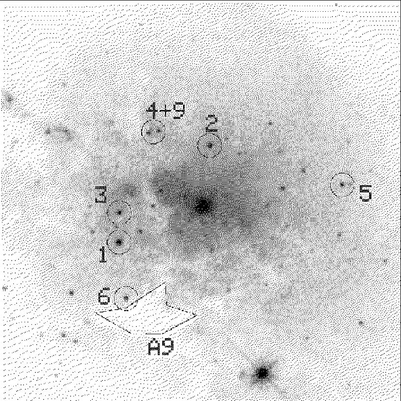
Figure 1: WFPC2 B image (F450W) of the inner 15 of NGC 1275. The 5 clusters for which we obtained spectra are circled. H3, also circled, was observed but its spectrum could not be successfully extracted because of its proximity to H1. Also marked is the dust region A9 studied by Nørgaard-Nielsen et al. (1993). The very bright object near the bottom of the image is a Galactic F–star. The image is oriented such that North is 138^o counter–clockwise from the vertical. East is 228^o clockwise from the vertical.

The galaxy spectrum of NGC 1275 consists of several components. The LV system, comprising the galaxy starlight and filamentary ionized gas, contains strong Balmer emission with broad [OIII] emission lines at a velocity close to the systemic velocity of the galaxy proper ($5264\rm\,km\,s^{-1}$). These emission lines become stronger toward the nucleus while widespread patchy dust appears to be significantly diminished very close to the nuclear region (See Nørgaard-Nielson et al. 1993 and Fig. 1/Plate ??). Superimposed on this LV material is the HV system with strong Balmer emission lines that are redshifted to a velocity of $\sim\,$$8000\rm\,km\,s^{-1}$. The emission lines for both systems vary significantly on spatial scales that are comparable to the sizes of the clusters themselves. This posed a serious challenge in determining an appropriate background subtraction procedure for extracting the cluster spectra. Additional challenges in reducing the data arose from instrumental limitations (discussed below) and the proximity of the cluster candidates to the bright galaxy nucleus. All the proto–globular cluster candidates we observed are within 5.3 of the galaxy center, corresponding to a distance of 1.9 $\rm h^{-1}\,kpc$ at the distance of NGC 1275. An individual cluster flux was $20\%$ of the background flux for the brightest objects we observed and $4\%$ for the faintest.

Because the grating blaze angle was quite red and detector was relatively insensitive to blue light, the system throughput at the blue end of the spectral range was quite poor. In addition, the spectral flat fields, taken with internal quartz–halogen lamps, contained spatially resolved artifacts due to illumination and reflection off the wire–bond region of the CCD. These artifacts did not appear in the data. Their presence in the spectral flats, combined with the low S/N in the blue, prevented flat–fielding the data on the blue end of the spectrum. Flat–fielding for the red end of the spectrum was done in the usual way. The 2–dimensional images were rectified in both the x and y directions using the IRAF tasks IDENT, REIDENT, FITCOORDS on spectra of comparison lamps and then the derived transformation was applied to the science images using the IRAF task TRANSFORM. The night sky background was subtracted using the IRAF task BACKGROUND. What remained were 2–dimensional images containing the spectra of the LV system, the HV system and the clusters.

The extraction procedure consisted of subtracting a representative galaxy spectrum from each of the 2–dimensional images, scaled to match the continuum level at the location of each cluster. Because of the multiple components and their variability on small spatial scales, the underlying galaxy light profile was not easily modeled from the 2–dimensional spectra alone. First attempts to determine the precise continuum level using only the LRIS spectral images, containing the combined galaxy, gas and cluster spectra, proved unsuccessful.

Ultimately, HST WFPC2 images of the region were used to model the galaxy profile at the position angle of each observation. The WFPC2 images were rotated to match the orientation of each LRIS spectral image and then convolved with a Gaussian function to mimic the seeing of the Keck observations. The WFPC2 images were then rebinned to match the plate–scale of the Keck spectral images. Finally, columns across the “slit” on the WFPC2 image were inspected to determine which combination of columns best matched the combined galaxy/gas/cluster light profile from the 2–dimensional Keck spectra. After finding the best match, the entire procedure was exactly repeated on the same WFPC2 image minus the clusters. The extracted light profiles from this second pass were used to determine the galaxy continuum at the location of the cluster. At most position angles the galaxy light profile revealed itself to be more complex than would have been possible to model using the 2–dimensional Keck spectra alone. Not surprisingly, this technique worked better for the higher S/N observations than for the lower S/N ones. For one position angle (158.1^o) we were not able to derive a satisfactory model of the galaxy light profile, so no spectra were extracted from that set of observations. Fortunately, the clusters observed at that position angle, H5 and H6 (identification from Holtzman et al. 1992), were observed at least at one other position angle. Once the underlying continuum level was determined, the major uncertainty (as far as spectral features are concerned) was in selecting an accurate “representative” galaxy spectrum from along the slit to subtract from the combined object+galaxy spectrum. Once the galaxy spectrum is removed a profile along the slit should ideally show only the light profiles of the clusters. In practice, there generally remained some residual galaxy light, attributable to an imperfect match between the representative galaxy spectrum and the true galaxy spectrum at the location of the cluster. Every effort was made to minimize this residual galaxy light, particularly in the region of the spectrum where the Balmer lines are located.

With the general galaxy spectrum removed, the task of eliminating the emission lines remained. It was necessary to perform these two operations (galaxy subtraction and emission line subtraction) separately because spatial variations in the strengths and ratios of the emission lines (for both the high and low velocity systems) do not correlate with spatial variations in the underlying galaxy spectrum/light profile. The technique for removal of the emission lines was simply to extract a sample of the emission lines from either side of the cluster along the slit and find the weighted average of the two samples that minimized the emission lines in the cluster spectra themselves. Having extracted the cluster spectra, flux calibration proceeded in the usual way. Corrections for atmospheric extinction and Galactic reddening (see Section 3) were made using the IRAF/NOAO routines STANDARD, SENSFUNC and CALIBRATE.

Of the eight objects observed, two (H12 and H17) were not detected above the noise and one (H3) was not sufficiently resolved from its nearest, and much brighter, neighbor (H1) for it to be extracted successfully. We will not consider these objects further. The spectra of the remaining 5 objects are shown in Fig. 2. Note that we have obtained a combined spectrum of H4 and H9 which are resolvable as two separate objects in the HST images but are not separable in the ground–based spectra. As explained above, the background contains several components each of which is spatially variable and the scales and amplitudes of the variations are different. Because the background subtraction process could not perfectly remove each component simultaneously, the continuum shapes of these spectra are not reliable and emission lines may have been under–subtracted (note that the background–subtraction process will not, in general, result in over–subtraction). Residual emission lines are particularly apparent in the lower signal–to–noise spectra. It is impossible to be absolutely certain that these emission lines do not belong to the objects themselves but we believe they are artifacts, since the velocities of the emission–line residuals are different from the cluster velocities by several hundred km/s. Moreover, these LV emission lines can be removed by adjusting the background mix (at the price of introducing other unacceptable features such as a negative continuum and/or absorption features from the now oversubtracted HV system), indicating that they belong to the background emission.

The clusters’ spectra do not resemble spectra of HII regions. All but the lowest signal–to–noise spectrum, that of H2, contain absorption features and a significant continuum component. The emission lines are demonstrably residuals from the background subtraction process. In the case of H2 where the continuum component is very weak, the presence of [NI] $\lambda 5199$ effectively rules out an HII region. [NI] $\lambda 5199$ is distinctly present in the spectrum of the nuclear region of the galaxy and H2 has the smallest radial distance from the nucleus of our entire sample, suggesting that the [NI] $\lambda 5199$ line in the spectrum of H2 is a residual from the imperfect background subtraction. We conclude that all 5 objects are bona fide clusters.

3 Photometry

There is some disagreement in the literature about the magnitudes and colors of the proto–globular cluster candidates. Richer et al. (1993) noted problems with the WFPC1 photometry of Holtzman et al. (1992) and Faber (1993) indicated that the CFHT photometry of Richer et al. (1993) must also be incorrect at some level. The photometric studies of Nørgaard-Nielsen et al. (1993) and Ferruit & Pécontal (1994) do not agree particularly well with either of the above nor with each other. We elected to use the WFPC2 images, taken from the HST archive, to derive our own B and R magnitudes for the clusters. Using circular apertures and a curve–of–growth type analysis we estimated total F450W and F702W magnitudes. These were converted into standard Johnson B and R magnitudes using the zeropoints and color transformations given in Holtzman et al. (1995). Our magnitudes and colors are presented in Table 2 along with those of Holtzman et al. (1992), Richer et al. (1993), Nørgaard-Nielsen et al. (1993) and Ferruit & Pécontal (1994). The Holtzman et al. V magnitudes have been corrected for the acknowledged factor of 2 error, i.e. they have been brightened by 0.75 mag (see Richer et al. 1993). Except for the H4+H9 clusters, the Ferruit & Pécontal R magnitudes are in excellent agreement with our WFPC2 R values. All the entries in Table 2 have been corrected for foreground Galactic extinction corresponding to $\rm E_{(B\!-\!V)}\!=\!0.17$ (Burstein & Heiles 1984) and A_B = 0.71, A_V = 0.54, A_R = 0.40 and A_I = 0.26.

Nørgaard–Nielson et al. (1993) modeled the dust extinction law and estimated A_V and A_I for 9 regions (designated A1–A9) in the galaxy lying between 4.7 and 23 from the galaxy nucleus. They found 0.20$<$$\rm A_{V}$$<$0.81 and 0.19$<$$\rm A_{I}$$<$0.69 for these regions. Fig. 1/Plate ?? is a WFPC2 B image of the inner $\sim\,$15 of NGC 1275. The dust region A9, which appears on the WFPC2 PC image, is marked on Fig. 1/Plate ?? along with the 5 clusters whose spectra are shown in Fig. 2. H3 is also marked but its spectrum could not be extracted because of its proximity to the much brighter H1. Although none of the clusters appears by eye to be positioned directly in a dust region as dense as A9 ($\rm A_{V}\!=\!0.35$), variations in the underlying background brightness can easily disguise the contrast with dense dust clumps, particularly for regions closer to the galaxy center. Interestingly, the three reddest clusters for which we obtained spectra are clearly more affected by dust than the others. H1 is superposed on a dust filament of width comparable to the size of the cluster. H6 and H4 are both located close to the apparent edges of dust regions. Of the bluer objects we observed, only H5 is in a region that is apparently unaffected by patchy dust.

To quantify these impressions we created a B-R color image using the HST data. For each cluster we measured the reddest color in the region adjoining the cluster, and the bluest color in the galaxy at the same radius as the cluster. The difference between the reddest and bluest color represents a rough value for the possible internal reddening for each cluster, assuming that the bluest color represents the true underlying color. These reddening estimates are included in Table 2. The bluest regions of the galaxy may themselves be reddened, and relatively uniformly distributed internal dust would not be detected by this method. Therefore the clusters could still be bluer than the bluest color limits we suggest.

The cluster apparent magnitude from the WFPC2 data can be used to derive a mass estimate. We used the population synthesis models of Fritze-v. Alvensleben & Burkert (1995) to determine how much a cluster will fade by the time it is $\sim$ 15 Gyr old. Assuming a present age of $\sim$ 400 Myr (see section 6), a true distance modulus of 34.23 for NGC 1275, a V-band M/L ratio of 2 for the clusters (if the clusters do indeed evolve into globular clusters they will have roughly this M/L ratio at $\sim$ 15 Gyr) and Galactic extinction of $\rm E_{(B\!-\!V)}\!=\!0.17$, we derive a mass of $\sim\,$2 x 10⁷ M_⊙ for the brightest cluster, H1. This is consistent with the value deduced by Holtzman et al. (1992). In section 6 we discuss the implications of color and reddening for age dating and formation scenarios for the clusters.

We measured the sizes of all 7 single clusters on the WFPC2 images to determine if the clusters are resolved. At the distance of NGC 1275 a typical Milky Way globular cluster (effective radius R_eff $\sim$ 3 pc, where R_eff is the half–light radius,. as defined as in Whitmore et al. 1993) would not be resolved, even with the $\sim\,$0.05 resolution of of the Planetary Camera (PC) on HST. At the distance of NGC 1275, one pixel on the PC corresponds to $\sim$17 pc so the largest Milky Way globular clusters R${}_{eff}\sim$ 10 pc would be barely resolvable. Using the method developed and calibrated by Miller et al. (1997) in their study of NGC 7252 young clusters, we have measured the FWHM and the magnitude difference between 0.5 and 3.0 pixels radius apertures and we conclude that none of these brightest NGC 1275 clusters are resolved.

4 Spectral Types and Equivalent Widths

The proto–globular cluster candidates were compared with standard star spectra covering a range of spectral types and luminosity classes. Ignoring the overall continuum shape, which we have argued is unreliable because of the background subtraction process and which may be subject to reddening effects (see section 3), the best visual match is with A0 to A3 dwarfs and class III giants. The match is illustrated in Fig. 3 in which selected comparison stars from the stellar library of Jacoby et al. (1984) are presented. The proto–globular cluster candidates are not well–represented by class I or II giant star spectra nor by spectra of stars of significantly cooler or hotter spectral classification. For instance, there are no obvious HeI lines which rules out the hottest stars. There is a hint of G–band contribution to the blue wing of H$\gamma$ which suggests an A rather than late–B classification. Types later than about A3 seems to be ruled out because of their relatively strong Ca K lines. To quantify these impressions we have measured equivalent widths in various A– and B–type main sequence stars from the compilations of both Jacoby et al. (1984) and Gunn & Stryker (1983).

It is worth noting here that there exist in the literature and in common use a number of alternative bandpass definitions and methods of measuring equivalent widths (EWs). The method employed in the Bruzual & Charlot (1993) models (hereafter BC93) gives systematically larger values of Balmer EWs than the Brodie & Hanes (1986) method (also adopted by Zepf et al. 1995). While the Brodie & Hanes bandpasses are well–suited to measuring features in old globular clusters and early–type galaxies, they are too narrow for measuring Balmer lines in young stellar populations where these features are relatively strong and broad. The algorithm employed in the BC93 models for measuring the Balmer line strengths is better suited to measuring the wide Balmer lines of young stellar populations. However, the choice of continuum level in the BC93 program is determined only by the flux values of the end points of the continuum bandpasses and can, therefore, be greatly affected by noise. This algorithm is not appropriate for low S/N spectra. For this reason we have employed Balmer line bandpass definitions that have been custom–defined for the purpose of studying young stellar populations. These bandpasses (referred to as LS indices after Linda Schroder who defined them) are provided in Table 3. The algorithm we use to determine the continuum level is based on the average flux value in the continuum bandpasses and so is better suited to low S/N spectra. The LS bandpasses have been chosen to agree well with the BC93 method when applied to the same high S/N spectra.

Bruzual and Charlot (1993) models reflecting changes described in Charlot, Worthey & Bressan (1996), were circulated in 1995. These newer models (hereafter BC95) return EW values measured from SEDs with 10 $\!{\rm\AA/pixel}$ resolution. This resolution is insufficient for accurate measurement of narrow–bandpass indices and, in any case, the very large widths of the Balmer lines in young stellar populations make the use of such narrow–bandpass indices inappropriate. The more appropriate BC95 and LS indices were measured on stellar spectra from the libraries of Jacoby et al. (1984) and Gunn & Stryker (1983) to produce a plot of equivalent width as a function of spectral type (Fig. 4). The Jacoby et al. spectra were first smoothed to match the 10 $\!{\rm\AA/pixel}$ resolution of the Gunn & Stryker spectra. As demonstrated in Fig. 4, the agreement between LS and BC95 indices is excellent for H$\beta$ and H$\delta$. The small systematic offset in the values of H$\gamma$ is due to the fact that the BC95 algorithm only uses the red side of the line when computing this equivalent width. This suppresses any effect from of the G–band, which is present just blueward of H$\gamma$. Both BC95 and LS indices are relatively insensitive to spectral resolution.

The horizontal lines in Fig. 4 represent the LS EW measurements of H1, for which we obtained the highest signal–to–noise data, and the arithmetic mean of 4 clusters. H2 was excluded from the mean since the Balmer line emission from the galaxy was clearly under–subtracted in that spectrum. H$\beta$ is subject to the greatest background subtraction uncertainties of all the Balmer lines in our spectral range because it is so strong in emission in the background spectrum. There is ample evidence in Fig. 2, especially in the lower signal–to–noise spectra, that H$\beta$ emission from the background has been under–subtacted. The residual emission serves to depress the mean EW for H$\beta$. Note that, in general, the background subtraction process was executed in such a way as to result in either correct or under–subtraction of the background emission lines rather than their over–subtraction.

Since the cluster spectra are integrated spectra, a perfect match with a single spectral type is not to be expected. Moreover, there is considerable scatter in Balmer EW measurements for different stars within a given spectral type, although these differences are generally comparable to our cluster measurement errors. However, the EWs confirm the visual impressions of the best matching spectral type from Fig. 2 and Fig. 3. Taking account of the absence of strong Ca K, which rules out later A–types, we conclude that the NGC 1275 proto–globular cluster candidates are dominated by early A–type stars with a best match at perhaps A0 or A1. This conclusion is supported by the stellar evolutionary modeling described in section 6.

Table 4 gives the LS EWs of H$\beta$, H$\gamma$ and H$\delta$ for the NGC 1275 proto–globular cluster candidates. For completeness, in Table 5 we provide EWs for H1 derived using narrow–bandpass indices, for direct comparison with the results of Zepf et al. (1995). The definitions of the Mgb and Fe 5270 features are from Faber et al. (1985), and the Balmer line bandpasses are those defined by Brodie & Hanes (1986).

5 Velocities

Velocities were determined from each unfluxed spectrum using the IRAF cross–correlation routine FXCOR. Velocities quoted in Table 6 are the average of the results of cross–correlation with 2 different, high signal–to–noise, A–star templates with small (absolute values of $<$$7\rm\,km\,s^{-1}$) heliocentric velocities, obtained from the Jacoby et al. (1984) library of stellar spectra plus a synthetic A–star template made by combining spectra from a large number of different A–stars. The cross–correlation was made over the region blueward of H$\beta$ to avoid bias from possible under–subtraction of the background emission lines. The Jacoby et al. spectra have a resolution of 4.5 Å so could, in principle, provide a velocity precision of $\sim$$30\rm\,km\,s^{-1}$. The results from the three templates agree quite well, differences being a small ($\sim$10–30%) fraction of the velocity error.

We exploit the presence of Balmer absorption in the underlying galaxy starlight to estimate the galaxy’s “local” line–of–sight velocity at the locations of the clusters. At each cluster location the cluster+galaxy+gas spectrum (from which the cluster spectra were eventually extracted) was cross–correlated against the A–star templates. Since the light from the clusters amounts to, at most, 20% of the total light producing these spectra, a cross–correlation that is restricted to the Balmer lines should give a reasonable estimate of the local bulk stellar velocity. The local velocity of the surrounding gas was estimated simply by measuring the line centers of the best Gaussian fits to the various emission line profiles in the cluster+galaxy+gas spectra. The local galaxy and gas velocities appear in Table 6. Excluding the composite object, H4+9, the mean difference between the velocities of the clusters and the local stellar velocity is 47$\pm$144$\rm\,km\,s^{-1}$. The mean difference between the velocites of the clusters and the local gas velocity is 50$\pm$101$\rm\,km\,s^{-1}$. There is no basis for preferentially associating the clusters with either the gas or the stars. None of the clusters is associated with the high velocity infalling material.

Zepf et al. (1995) found velocity differences for H1 “relative to the emission line gas” of –120 and $-140\rm\,km\,s^{-1}$ at to two different position angles. Our results also show a comparable blue-shift of H1 with respect to the [OIII] emission lines, but not with respect to [OI] $\lambda 6300$ or H$\beta$. It is not surprising that the gas velocities yielded by these features are mildly discrepant. Due to the wavelength dependence of dust scattering properties, measuring features at different wavelengths may be probing to different depths along the line–of–sight. At the location of H2 and H5, the [OIII] emission lines in the gas spectra appear to contain two velocity components with the weaker component located blueward of the main component. In these cases we measured the velocities of both components. The resulting velocities are listed in Table 6.

We find a velocity dispersion of 244$\pm$99$\rm\,km\,s^{-1}$ for the clusters (excluding the composite object, H4+9), which, although very poorly constrained, seems to be somewhat lower than that of globular cluster systems in dominant central galaxies (e.g. M87, Cohen & Rhyzhov 1997; NGC 1399, Grillmair et al. 1994, Kissler-Patig et al. 1998, Minniti et al. 1998). Note that the NGC 1275 clusters are all very close to the galaxy nucleus (within $\sim\,$2 kpc). The central stellar velocity dispersion of NGC 1275 has not been accurately measured but Lazareff et al. (1989) derived a value of $290\rm\,km\,s^{-1}$ by modeling the mass distribution in the galaxy’s potential well. Recall that Lazareff et al. found a velocity dispersion of $\sim\,$$113\rm\,km\,s^{-1}$ for the CO gas in the center of NGC 1275, presumed to be associated with the H$\alpha$ filaments and the clusters. This value is marginally consistent with the cluster velocity dispersion estimates, given the size of the errors.

The arithmetic mean velocity of the clusters, excluding H4+9, is 5329$\pm$121$\rm\,km\,s^{-1}$, consistent with the galaxy velocity of $5264\rm\,km\,s^{-1}$ measured by Strauss et al. (1992) as well as the local galaxy velocity determined from the background spectrum. The error quoted is the standard error of the mean.

6 Comparison with Star Clusters and Stellar Evolutionary Models

6.1 Star Clusters

Bica & Alloin (1986) present integrated spectra for star clusters covering a wide range of ages and metallicities. Their plots of index EW versus metallicity confirm the expected lack of sensitivity to metallicity of line features in young cluster spectra.

Table 7 is a list of the LS Balmer line EWs for the spectra of selected young clusters from the Bica & Alloin data base, as tabulated by Leitherer et al. (1996). The best match is obtained for clusters having ages of 200–500 Myr, though the NGC 1275 clusters have EWs which are larger than those for any cluster in the Bica & Alloin sample, irrespective of age or metallicity. This suggests that the NGC 1275 clusters are not well–represented by Magellanic Cloud young or intermediate age clusters, nor by Galactic globular or open clusters, a conclusion that is confirmed by visual inspection of the spectra of the Bica & Alloin objects (Fig. 3).

6.2 Bruzual & Charlot Models

BC95 stellar evolutionary models at solar metallicity were used to generate plots of H$\beta$, H$\delta$ and H$\gamma$ EWs as a function of age. These are shown in Fig. 5. The horizontal lines in these plots represent the EWs measured for the highest signal–to–noise cluster, H1, and the arithmetic mean of 4 clusters. Again, H2 was excluded from the mean because significant residual emission lines from the background galaxy are present in its spectrum. Note that, as mentioned in section 4, the mean EW of H$\beta$ is likely to be somewhat depressed due to under–subtraction of the background H$\beta$ component. This may be true for H1 but is especially relevant for the lower signal–to–noise spectra.

Initially a Salpeter IMF ($\rm 0.1\!-\!125\,M_{\odot}\,\,$, X=1.35) was adopted and a delta function burst of star formation at t=0 years was assumed. The relatively low S/N of our spectra (with the exception of H1) prevents us from using the exact prescription of BC95 for a comparison of the clusters’ Balmer line strengths with the model predictions. The smoothing and rebinning to very low resolution (10 $\!{\rm\AA/pixel}$) combined with the algorithm’s “end–point only” determination of the continuum flux can produce quite spurious results for low S/N spectra. For this reason we adopted the index measurement method outlined in Brodie and Huchra (1990) using the LS bandpass definitions decribed in section 4. Fig. 4 demonstrates that, for high S/N spectra, this method and the BC95 algorithm produce very similar results. For low S/N spectra this method allows a much more accurate determination of the continuum flux and therefore provides the most robust comparison with the models.

In Fig. 5 the lines representing H1, the cluster with by far the highest signal–to–noise spectrum, do not intersect the Salpeter IMF curves. It is possible to force an intersection for H$\beta$  (known to be artifically depressed) and barely possible for H$\delta$ (which is in the lowest signal–to–noise portion of the spectrum) by pushing both the EWs systematically lower towards the limit of their error bars. The value for H$\gamma$, arguably the best–determined EW, is more than two standard deviations away from the maximum of the Salpeter curve. The sample mean EWs for H$\gamma$ and H$\delta$ also do not intersect the Salpeter IMF curves. A shift towards the lower limit of its error bar does allow an intersection for H$\delta$ but not for H$\gamma$. The H$\beta$ measurement is included for completeness but is not reliably enough determined in these low signal–to–noise spectra to be a useful constraint on the models.

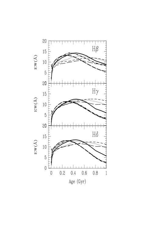
Figure 6: The time evolution of Balmer line equivalent widths for a simple stellar populations of various metallicities, produced by the preliminary BC97 models. For ages less than $\sim\,$0.5 Gyr, H$\gamma$ gives the tightest constraint on age, if the metallicity is unknown. This figure demonstrates the possible spread in Balmer line equivalent widths that can be attributed to metallicity differences.

The latest, albeit preliminary, Bruzual and Charlot (1997) models (hereafter BC97) allow metallicity to be varied in discrete steps (corresponding to [Fe/H] = –1.7, –0.7, –0.4, 0.0, 0.4 and 0.7) while earlier versions forced the assumption of solar metallicity for the system. These BC97 models were kindly released to us in preliminary form in advance of publication. The theoretical input spectra used in BC97 have a substantially lower resolution (20 $\!{\rm\AA/pixel}$) than the empirical spectra used in BC95. This has caused (at the time of this writing) a systematic offset from the BC95 models, especially at young ages, in the sense that the BC97 models return higher values of Balmer line EWs. Nevertheless, the preliminary models can adequately demonstrate the range of EWs that can be produced by varying metallicity. Fig. 6 shows the Balmer line EWs versus age for the range of metallicities provided in the BC97 models. If the metallicity is unknown, H$\gamma$ gives the tightest constraint on age, for ages $<$500 Myrs, owing to its small spread in EW for populations of different metallicity. For each Balmer line the maximum value of the EW occurs at solar metallicity for ages less than 500 Myr. Clearly, the solid curves in Fig. 5 (which represent solar metallicity) cannot be brought into agreement with the values measured for the clusters simply by allowing metallicity to vary. Except for the artifically depressed mean EW of H$\beta$, the Balmer line EWs of the clusters are larger than any returned by the BC models at any metallicity and agreement can only be achieved by systematic downward shifts of all the Balmer EWs.

It is worth noting here that the BC93 models and later variants suffered from an error which transposed the column labels on the output of EW values of H$\delta$ and H$\gamma$. (Bruzual, 1997). This has been corrected in our plots. Both Zepf et al. (1995) and Schweizer & Seitzer (1993) compare their measurements of Balmer line EWs in proto–globular cluster candidates equivalent widths from these models. Both note that the (BC93, solar metallicity) models are unable to produce EWs as strong as those they observed.

Having established that the large Balmer line EWs in the cluster spectra are not reproduced by varying metallicity in the standard models, we now explore the possibility that the IMF of these clusters is different from the standard IMF and specifically that it is skewed to high masses. All versions of the Bruzual and Charlot models allow for the adoption of Salpeter (1955) or Scalo (1986) IMFs but neither of these is consistent with the observed Balmer line strengths. The input SEDs for the Bruzual and Charlot models, as distributed, do not allow for variations in the slope of the IMF, nor can the range of allowed masses be specified arbitrarily. However, Bruzual and Charlot kindly provided us with an input SED for their models, generated originally for other purposes, which corresponds to a solar metallicity IMF truncated to include only $\rm 2\!-\!3\,M_{\odot}\,\,$stars, i.e. it has a low mass cut–off at 2 M_⊙ and a high mass cut–off at 3 M_⊙. This essentially corresponds to a population of pure A stars. We have adopted this SED to simulate a flatter IMF. As is clear from Fig. 5, this model reproduces the strong Balmer line EWs of the clusters and these are consistent with each other in predicting an age of $\sim$$\rm 425\!-\!500\,Myr$ for all the clusters (with the mean H$\beta$ exception noted above).

This age estimate is consistent with general arguments based on main sequence lifetimes for early A–type stars. Poggianti & Barbaro (1997) confirm that the maximum Balmer line EWs occur in A0V–type stars. A0 star masses are estimated to be anywhere in the range $\rm 2.2\!-\!3.5\,M_{\odot}\,\,$(e.g. Allen 1974, Straizys & Kuriliene 1981). If higher mass stars are no longer present in significant numbers, a crude age constraint can be determined from the duration of the H–burning phase of $\rm 2.2\!-\!3.5\,M_{\odot}\,\,$stars. Such stars are predicted to stay on the main sequence for $\sim\,$$\rm 0.2\!-\!0.7\,Gyr$, depending on the isochrones adopted and the metallicities assumed (e.g. Schaller et al. 1992)

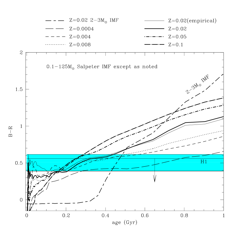
Figure 7: ($\rm B\!-\!R$) color vs. Age produced by the BC97 preliminary models. The color of H1, uncorrected for internal reddening, is represented by a horizontal line. A downward–pointing arrow indicates the effect of the estimated internal reddening, calculated from the HST images as described in section 3. The possible range of the average color of the 5 clusters in the sample is shown as a shaded region delimited by horizontal lines representing colors corrected and uncorrected for internal reddening.

Preliminary BC97 models for ($\rm B\!-\!R$) as a function of age are shown in Fig. 7. Since the ($\rm B\!-\!R$) colors measured from the empirical SEDs of the older models and the theoretical SEDs of the newest models appear to be consistent with each other for this broad–band color, we have illustrated the dependence at all available metallicities for the standard IMF (0.1–125 M_⊙) models. Also shown is the $\rm 2\!-\!3\,M_{\odot}\,\,$model at solar metallicity. In Fig. 7 the color of H1, uncorrected for internal reddening, is represented by a horizontal line. A downward-pointing arrow indicates the effect of the estimated internal reddening, calculated from the HST images as described in section 3. The average color of the 5 clusters in the sample, corrected and uncorrected for internal reddening, is also shown.

From this figure we conclude that the most probable age of H1, deduced from its color and the $\rm 2\!-\!3\,M_{\odot}\,\,$model is in the range 425–475 Myr, depending on the extent of the internal reddening. The corresponding age range deduced from the average cluster colors is 400–475 Myr. Note that the age derived from the color is consistent with the age deduced from the Balmer line measurements.

If a standard (Salpeter) IMF is assumed, for all but the lowest metallicity models, the age estimate drops to 400 Myr for the uncorrected color and less if any internal reddening is present. The age estimate drops to an untenable (in view of the spectral signature) 100 Myr if the full internal reddening estimate is applied. We have argued that the majority of the clusters are likely to be suffering significant internal reddening. Moreover, significantly sub–solar metallicities can be ruled out for ages as young as those derived from the EW measurements.

Taken as a whole, then, the cluster data appear to be more compatible with a truncated and/or flattened IMF than with a Salpeter IMF. In particular, age estimates from both EW and color measurements are mutually consistent without the need to impose systematic shifts of the measured values or discount internal reddening.

Although the agreement of our cluster data with the $\rm 2\!-\!3\,M_{\odot}\,\,$model suggests that the IMF of the clusters may be relatively flat, i.e. skewed to high masses, it does not, by itself, set any constraints on the nature of the IMF above 3 M_⊙. After $\sim\,$400 Myr, only A–stars will be left in the clusters regardless of the initial presence or absence of higher mass stars. However, the characteristics of an original population of high mass ( $>$ 3 M_⊙) stars, if any, can in principle be deduced because such stars cannot be allowed to disrupt the clusters prior to 400 Myr. In other words, the amount of mass lost from the clusters caused by the evolution of massive stars must be small enough that the clusters do not become unbound. Note too that, with a 2 M_⊙ lower mass cut–off, these clusters would fade away extremely quickly (in $\sim\,$10⁹ yr), assuming they manage to avoid disruption. Future modeling efforts will explore variations in the IMF slope and perhaps a variety of mass cut–offs in an attempt to reproduce the observations even more closely.

6.3 Fritze-v. Alvensleben and Kurth Models

Fritze-v. Alvensleben & Kurth (1997, hereafter FK) kindly compared our H1 spectrum with their models. Interestingly, the FK models can reproduce the observed H$\beta$ and H$\gamma$ EWs without the need to invoke a non–standard IMF, although the agreement with H$\delta$ is less good.

Table 8 gives the Balmer line EWs and colors measured from model SEDs of various ages. FK models in the range $\rm 200\!-\!500\,Myr$ provide a reasonable fit to the observed EWs with closest agreement for the 350 Myr model. For an age of 350 Myr, the mass deduced for this cluster is $\sim\,$10⁷ M_⊙. If the cluster is older the mass estimate will increase, if younger it will decrease. According to the FK models, a 400 Myr old cluster will fade by 3.4 magnitudes in 15 Gyr while a 250 Myr old cluster will fade by 3.8 magnitudes (O. Kurth, private communication). The current absolute B magnitude of H1 is –15.5, so in 15 Gyr it will have M_B $\sim\,$–11.9, which is comparable to the brightest globular clusters in M31, M87 and NGC 1399. H1 is by far the brightest of the proto–globular cluster candidates but it is clear on the basis of their luminosities, and hence their masses, that none of these objects would be defined as an open cluster.

The unreddened color predicted by the 350 Myr FK model is ($\rm B\!-\!R$)₀=0.44. The B-R color of H1 is 0.56, uncorrected for internal reddening, and is 0.24 if corrected for the value of extinction estimated in the immediate vicinity of the cluster for the dust lane in which H1 appears to lie. The model continuum is too red compared to the observed spectrum. We argued previously that the precise continuum shapes in the observed spectra are poorly defined because they are dependent on the background subtraction process. However, Fig. 2 and Fig. 3 indicate that the observed continuum shape is too red for the inferred spectral type, rather than too blue. In addition, no correction has been made for internal reddening. For these reasons, we infer that the true continuum shape of H1 is bluer than that appearing in Fig. 2 and that appropriate corrections (for background subtraction inaccuracies and internal reddening) would act to increase the discrepancy between the model and the observation. This discrepancy is in the sense that the model predicts too much red light and is thus consistent with the suggestion that the cluster IMF is flatter than a Salpeter IMF.

It is unclear why the BC95 and FK models give such different EW results. Both use the Padova evolutionary tracks (Bressan et al. 1993) but there are subtle differences between the two, such as the details of the template spectra adopted.

6.4 Metallicity

Table 9 compares the strengths of Mg, Fe and Na features in the spectrum of H1 with corresponding values from the 350 Myr FK models at various metallicities. As expected for a young stellar population, the weak metal lines are of little value in deducing the overall metallicity. However, despite the large errors, it is clear that Na is significantly overabundant compared to its solar value. The error on Mg is too large to judge its strength clearly but it too may be overabundant. We note that Na and Mg overabundances have been seen in giant elliptical galaxies (Worthey et al. 1992) and in a small subset of globular clusters in NGC 1399 (Kissler-Patig et al. 1998). Worthey et al. suggest various mechanisms for producing the Mg/Fe enhancements seen in the gE galaxies, one of which is a flat IMF.

7 Discussion

If we assume that the clusters in our sample are representative of the system of proto–globular cluster candidates as a whole, we can draw some interesting conclusions from our results which pertain to our understanding of the process of globular cluster formation and set some constraints on the origins of globular clusters.

The mean velocity of the clusters is consistent with the velocity of the main body of the galaxy and their velocity dispersion is 244$\pm$99$\rm\,km\,s^{-1}$. This dispersion is on the low side for globular clusters in giant elliptical galaxies. It has been argued that the clusters are associated with the LV filaments, which in turn are associated with the CO gas. Both the filaments and the CO gas are presumed to have been formed in the cooling flow. The cooling time for the CO gas is $\sim\,$10 Myr, very similar to the X–ray cooling time in these innermost regions (Mushotzky et al. 1981). Since we can rule out ages this young for the clusters, we can rule out their formation in a continuous cooling flow and possibly, by association (if the CO gas and the clusters are indeed spatially linked), the formation of the LV filaments and the CO gas in the cooling flow.

H$\alpha$ images (Lynds 1970; Baade & Minkowski 1954) indicate that the extent of the filaments is 2–2.5 for the LV system and 1–1.5 for the HV system. Assuming a “normal” (King, de Vaucouleurs, or Hubble–like) density profile for the H$\alpha$ material would suggest an effective radius of perhaps 20–30 and a core radius of even less. The scale of the filaments might be similar to the scale of the proto–globular cluster candidates. The cooling flow radius is $\sim\,$5.5 (Allen & Fabian 1997) which is a factor of 60 larger than the radius of our sample and a factor of 20 larger than the entire sample of proto–globular cluster candidates. Moreover, a cooling flow scenario requires star formation with a steep IMF to account for the absence of observed high–mass stars in conjunction with the deduced $>$ $\rm 400\,M_{\odot}\,yr^{-1}$ star formation rate. If confirmed, the flat IMF (biased against low mass stars) deduced for the clusters would be further evidence against their association with the cooling flow. All this argues positively for a merger origin for the filaments and the clusters.

The clusters show a remarkable degree of central concentration. From the work of Holtzman et al. (1992) and Richer et al. (1993) we know that all the currently–identified proto–globular cluster candidates lie within $\sim\,$8 kpc of the nucleus. Richer et al. (1993) noted that the brighter clusters were more centrally located than the fainter ones. Those in our study, i.e. the brighter candidates, lie within $\sim\,$1.5 kpc of the nucleus. By contrast, the old globular clusters lie within about 30 kpc of the nucleus (Kaisler et al. 1996), so the old and young clusters are very differently distributed. This degree of central concentration appears to be greater than that seen for metal–rich globular clusters in any “normal” elliptical galaxy.

It is not clear why formation in a merger would preferentially form clusters only in the central few kpc if star formation is triggered in chaotically distributed shocks. However, it is to be expected that gas from merging galaxies will be channeled rapidly to the center (Barnes & Hernquist 1996 and references therein) where it can form stars very soon after the onset of the merger event. It is unlikely that widespread shocks from merging galaxies could have produced these clusters both on the grounds of their central concentration and because their velocity dispersion may be relatively low. If the clusters were formed further out in the galaxy and later fell into the center, a high velocity dispersion would be expected. In fact, it might be difficult to find a mechanism for moving the clusters nearer to the galaxy center since dynamical friction is not likely to be effective at these masses, although they might conceivably have been associated with an infalling galaxy. In any case, we can conclude that they actually formed very close to the galaxy center. A cooling flow or central accumulation of merger gas is then more appealing in this regard because the gravitational potential definitely steepens rapidly near the galaxy center and objects formed in this potential would acquire the mean velocity of the galaxy. It will be of great interest to obtain similar high–quality spectra of proto–globular cluster candidates in other interacting galaxies, especially ones without cooling flows.

If mergers are to contribute significantly to high S_N globular cluster systems (although see Forbes, Brodie & Grillmair 1997 for arguments against that idea) and mergers produce very centrally concentrated globular clusters, some mechanism has to be invoked to redistribute the clusters to resemble the observed spatial distributions in normal cluster systems. For example, in M87 (Grillmair et al. 1986 and Lauer & Kormendy, 1986) and in NGC 1399 (Kissler-Patig et al. 1997) it has been established that the globular cluster systems are more diffuse than the galaxy light. A similar argument can be made for centrally concentrated objects formed from a cooling flow.

The crossing time for objects with $\sim\,$$200\rm\,km\,s^{-1}$ velocity dispersion with a radius of 8 kpc (the radial extent of whole proto–globular cluster candidate sample) is $\sim\,$40 Myr, or a factor of 10 less than their age. Their survival in the galaxy center must indicate that they are in virial equilibrium, unless the velocity dispersion measurement is unrepresentative because of the very small sample of velocities.

We have found evidence that these clusters have an IMF that is flat (skewed to high masses or biassed against low masses) compared to a standard IMF. The low-mass stellar component may be weak or possibly absent in these objects and, in order to avoid disruption long enough to survive to $\sim$400 Myr, there are restrictions on the high mass component.

Interestingly, recent work by Padoan et al. (1997) provides a natural framework for such a result if star formation is driven by random supersonic flows. They predict that starburst regions should have flatter IMFs with a more massive low–mass cut-off because of their higher mean temperatures. Based on core–radius measurements, Elson, Freeman & Lauer (1989) report evidence for a flatter IMF in their study of the core radii of young clusters in the Large Magellanic Cloud. However, as already noted, the spectra of LMC clusters are not similar to those of the NGC 1275 young clusters.

8 Summary and Conclusions

The clusters we have studied are not HII regions and their integrated spectral properties do not resemble those of young or intermediate age Magellanic Cloud clusters or Milky Way open clusters.

The clusters’ Balmer line strengths appear to be too strong to be consistent with any of the standard Bruzual and Charlot evolutionary models at any age or metallicity. If the Bruzual and Charlot models are adopted, an IMF which is skewed to high masses provides a more internally consistent fit to the spectral and photometric data. A truncated IMF with a mass range of $\rm 2\!-\!3\,M_{\odot}\,\,$ adopted to mimic a flatter IMF, reproduces the observed EWs at $\rm 425\!-\!500\,Myr$ and the cluster colors predict ages of $\sim\,$$\rm 400\!-\!475\,Myr$ for this mass range.

The FK models are better able to reproduce the observed Balmer line strengths for a solar metallicity cluster with an age of 350 Myr and a standard (Salpeter) IMF, although the model continuum is too red compared to the observed spectrum. The continuum discrepancy between the model and the observation is in the sense that the model predicts too much red light and thus is also consistent with the suggestion that the cluster IMF is relatively flat.

Key properties of the clusters, in addition to their possibly flat IMF, are their extremely centrally concentrated spatial distribution, their velocity dispersion of 244$\pm$99$\rm\,km\,s^{-1}$ and their age of $\sim\,$450 Myr.

Formation in a continuous cooling flow appears to be ruled out since the age of the clusters is much larger than the cooling time of the molecular gas (assuming that the molecular gas is associated with the cooling flow), the spatial scale of the clusters is much smaller than the cooling flow radius, and the deduced star formation rate in the cooling flow favors a steep rather than a flat IMF.

A merger would have to produce clusters only in the central few kpc, presumably from gas from the merging galaxies which is channeled rapidly to the center. Widespread shocks from merging galaxies cannot have produced these clusters. If they were formed further out in the galaxy and later fell into the center (by some unspecified mechanism), a high velocity dispersion would be expected.

The crossing time of the clusters is only $\sim\,$40 Myr. Their survival to $\sim\,$400 Myr indicates that they must be in virial equilibrium if the observed velocity dispersion is representative of the whole young cluster population.

Regardless of their origin, these objects are not distributed like old globular clusters in central cD galaxies where the globular clusters are significantly more diffuse than the galaxy light.

The clusters appear to have formed in a discrete event some 450 Myr ago. This event might have been induced by a merger which provided the fuel for a short–lived gas infall episode. With a small or absent low mass stellar component, these objects would fade away very rapidly (in $\sim\,$$10^{9}$ yr), assuming they can avoid disruption in the later stages of stellar evolution. More data and further modeling, especially to determine the slope and/or cut–off parameters of the IMF, are required to ascertain whether or not they will eventually evolve into objects we would regard as bona fide globular clusters.

REFERENCES

Arnaud, K.A., et al. 1994, ApJ, 436, L67
Ashman, K.M., & Zepf, S.E. 1992, ApJ, 384, 50
Allen, C.W. 1974, Astrophysical Quantities, 3rd Ed., (The Athalone Press, London), p. 208
Allen, S.W., & Fabian, A.C. 1997, MNRAS, 286, 583
Allen, S.W., Fabian, A.C., Johnstone, R.M., Nulsen, P.E.J., & Edge, A.C. 1992, MNRAS, 254, 51
Baade, W., & Minkowsky, R. 1954, ApJ 119, 215
Barnes, J.E. & Hernquist, L. 1996, ApJ 471, 115
Bica, E., & Alloin, D. 1986, A&A, 162, 21
Blakeslee, J. 1996, PhD thesis, M.I.T.
Bressan, A., Fagotto, F., Bertelli, G., & Chiosi, C. 1993, A&AS, 100, 647
Brodie, J.P., & Hanes, D.A. 1986, ApJ, 300, 258
Brodie, J.P., & Huchra, J.P. 1990, ApJ, 362, 503
Burstein, D., & Heiles, C. 1984, ApJS, 54, 33
Burstein, D., Faber, S., Gaskell, M., & Krumm, N. 1984, ApJ, 287, 586
Bruzual, G., & Charlot, S. 1993, ApJ, 405, 538
Bruzual, G., & Charlot, S. 1997, in preparation
Bruzual, G., 1997, private communication
Charlot, S., Worthey, G., & Bressan, A. 1996, ApJ, 457, 625
Cohen, J.G., & Rhyzhov, A.S. 1997, AJ 486, 230
Elson, R.A.W., Freeman, K.C. & Lauer, T.R. 1989 ApJ 347, L69
Faber, S., Friel, E.D., Burstein, D., & Gaskell, C.M. 1985, ApJS, 57, 711
Faber, S. 1993, The Globular Cluster–Galaxy Connection, ASP conf. series Vol. 48, eds. G. Smith, & J. Brodie, p.601
Fabian, A.C., Nulsen, P.E.J., & Canizares, C.R. 1984, Nature, 310, 733
Fabian, A.C., Hu, E.M., Cowie, L.L., & Grindlay, J. 1981, ApJ, 336, 734
Ferruit, P., & Pécontal, E. 1994, A&A, 288, 65
Forbes, D., Brodie, J.P., & Huchra, J.P. 1996, AJ, 112, 2448
Forbes, D., Brodie, J.P., & Grillmair, C. 1997, AJ, 113, 1652
Fritze-v. Alvensleben, U. & Burkert, A. 1995, A&A, 300, 58
Fritze-v. Alvensleben, U. & Kurth, O. 1997, in preparation
Grillmair, C., Pritchet, C., & van den Bergh, S. 1986, AJ, 91, 1328
Grillmair, C., et al. 1994, ApJ, 422, L9
Gunn J.E., & Stryker, L.L. 1983, ApJS, 52, 121
Harris, W.E. 1991, ARA&A, 29, 543
Holtzman, J.A., et al. 1992, AJ, 103, 691
Holtzman, J.A., et al. 1995, PASP, 107, 1066
Holtzman, J.A., et al. 1996, AJ, 112, 416
Holtzman, J.A., et al. 1998, in preparation
Johnson, H.L. 1966, ARAA, 4, 193
Jacoby, G.H., Hunter, D.A., & Christian, C.A. 1984, ApJS, 56, 278
Kaisler, D., Harris, W.E., Crabtree, D.R. & Richer, H.B. 1996, AJ, 111, 2224
Kissler-Patig, M., Kohle, S., Hilker, M., Richtler, T., Infante, L., Quintana, H. 1997, A&A, 319, 470
Kissler-Patig, M., Brodie, J.P., Schroder, L.L.,Forbes, D.A., Grillmair, C.G., & Huchra, J.P. 1998, AJ 115, 105
Lauer, T., & Kormendy, J. 1986, ApJ, 303, L1
Lazareff, B., Castets, A., Kim, D.W., & Jura, M. 1989, ApJ, 336, L13
Leitherer, C. et al. 1996, PASP, 108, 996
Lynds, C.R. 1970, ApJ, 159, L151
Miller, B.W., Whitmore, B.C., Schweizer, F., & Fall, S.M. 1997, AJ in press
Minkowski, R. 1957, Radio Astronomy, IAU Symposium No. 4, ed. H.C. van de Hulst (Cambridge University Press, Cambridge), Vol. 107
Minniti, D., Kissler-Patig, M., Goudfrooij P., & Meylan, G. 1998, AJ, 115, 121
Mushotzky, R. 1992, Clusters and Superclusters of Galaxies, ed. A.C. Fabian (Kluwer, Dordrecht), p. 91
Mushotzky, R., Holt, S.S., Boldt, E.A., Selemitsos, P.J., & Smith, B.W. 1981, ApJ 244, L47
Nørgaard-Nielsen, H.U., Goudfrooij, P., Jorgensen, H.E., & Hansen, L. 1993, AA, 279, 61
Oke, J.B., et al., 1995, PASP 107, 375
Padoan, P., Nordlund, A., & Jones, B.J.T. 1997, MNRAS 288, 145
Poggianti, B.M., & Barbaro, G. 1997, A&A, in press
Richer, H.B., Crabtree, D.R., Fabian, A.C., & Lin, D.N.C. 1993, AJ, 105, 877
Rieke, G.H., & Lebofsky, M.J. 1985, ApJ, 288, 618
Salpeter, E.E. 1955 ApJ, 121, 61
Scalo, J.M. 1986, Fundamentals of Cosmic Physics, 11, 3
Schaller, G., Schaerer, D., Meynet, G., & Maeder, A. 1992, A&AS, 96, 269
Schweizer, F., & Seitzer, P. 1993, ApJ, 417, L29
Schweizer, F. 1987, Nearly normal galaxies: From the Planck time to the Present, Proceedings of the Eighth Santa Cruz Summer Workshop in Astronomy and Astrophysics, ed. S. Faber (Springer-Verlag, New York), p.18
Smith, E.P. et al. 1992, ApJ, 395, L49
Straizys, V., & Kuriliene, G. 1981, Ap&SS, 80, 353
Strauss, M., Huchra, J.P., Davis, M., Yahil, A., Fisher, K., & Tonry, J. 1992, ApJS, 83, 29
Straziys, V. & Kuriliene, G. 1981, Ap&SS, 80, 353
Whitmore, B., Schweizer, F., Leitherer, C., Borne, K., & Robert, C. 1993, AJ, 106, 1354
Whitmore, B.C., & Schweizer, F. 1995, AJ, 109, 960
West, M.J., Cote, P., Jones, C., Forman, W., & Marzke, R.O. 1995 ApJ 453, L77
Worthey, G., Faber, S.M., & Gonzales, J.J. 1992, ApJ 398, 69
Zepf, S.E., Carter, D., Sharples, R.M., & Ashman, K.M. 1995, ApJ, 445, L19
Zabludoff, A., Huchra, J.P., & Geller, M. 1990, ApJS, 74, 1

Table 1: Observational Data

Cluster	Slit	Integration	Dates
ID	PA	Time	Observed
(1)	(2)	(3)	(4)
H1	153.0	900	Dec 01
	46.7	6300	Nov 30
H2	113.5	3200	Nov 30
H3	46.7	6300	Nov 30
H4+H9	113.5	3200	Nov 30
H5	113.5	3200	Nov 30
	158.1	1800	Dec 01
	140.0	900	Dec 01
H6	46.7	6300	Nov 30
	158.1	1800	Dec 01
H12	77.4	4500	Dec 01
H17	77.4	4500	Dec 01

lrccrrrcrlcrrrr 0pc 2 Magnitudes^∗ and Colors & This F & P Richer Holtzman Nørgaard
Paper (1994) et al. (1993) et al. (1992) et al. (1993)
(1) (2) (3) (4) (5)

Cluster ID B R R B V I V R V I
H1 19.00 18.44 18.50 18.98 18.65 18.38 18.41 18.22 18.36 17.73 $\sigma_{H1}$ 0.15   0.15 0.16 0.01   0.03 0.02   0.02 0.02 0.01 0.00 H2 20.18 19.53 19.54 20.11 19.89 19.53 19.51 19.38 19.95 19.43 $\sigma_{H2}$ 0.15   0.15 0.16 0.07   0.09 0.09   0.08 0.14 0.02 0.02 H3 20.05 19.35 19.62 20.34 19.66 19.48 19.41 19.23 $\sigma_{H3}$ 0.15   0.15 0.35 0.11   0.04 0.04   0.08 0.05 H5 20.57 20.15 20.71 20.36 20.05 20.11 20.01 20.96 20.56 $\sigma_{H5}$ 0.15   0.15 0.05   0.06 0.03   0.04 0.06 0.03 0.05 H6 20.76 20.04 20.63 20.46 19.91 20.21 20.02 20.12 19.45 $\sigma_{H6}$ 0.15   0.15 0.19   0.08 0.03   0.06 0.08 0.02 0.00 H4+H9^∗∗ 19.72 19.07 20.04 $($19.91 20.52 20.70$)$ $($19.48 19.30$)$ $($20.21 19.74$)$ $\sigma_{H4+H9}$ 0.15   0.15 0.47 $($0.06   0.18 0.22$)$ $($0.08 0.11$)$ $($0.02 0.02$)$ B–R E_(B-R) B–V V–I V–R V–I H1 0.56 0.32 0.33 0.27 0.19 0.63 $\sigma_{H1}$ 0.21 0.03 0.04 0.03 0.01 H2 0.65 0.18 0.22 0.36 0.13 0.39 $\sigma_{H2}$ 0.21 0.11 0.13 0.16 0.03 H3 0.70 0.23 0.68 0.18 0.18 $\sigma_{H3}$ 0.21 0.12 0.06 0.09 H5 0.42 0.03 0.35 0.31 0.10 0.40 $\sigma_{H5}$ 0.21 0.08 0.07 0.07 0.06 H6 0.72 0.25 0.17 0.55 0.19 0.67 $\sigma_{H6}$ 0.21 0.21 0.09 0.10 0.02 H4+H9 0.65 0.33 (-0.60 -0.18) (0.18) (0.47) $\sigma_{H4+H9}$ 0.21 (0.19 0.28) (0.14) (0.03) NOTES *Magnitudes have been corrected for foreground Galactic extinction (i.e. A${}_{B}=0.71$, A${}_{V}=0.54$, A${}_{R}=0.40$ and A${}_{I}=0.26$). The Holtzman et al. values have been corrected for the acknowledged (Richer et al. 1993) factor of 2 error, i.e. 0 .75 mags. **The objects H4 and H9 are unresolved from the ground. Ferruit & Pécontal (1994) note this and give a magnitude for H4+H9. Richer et al. (1993), however, list magnitudes only for H9, whereas Nørgaard–Nielsen et al. (1993) list magnitudes only for H4. We have placed those magnitudes on the line for H4+H9, since each is bound to include both objects. The entries for H4+H9 in the Holtzman et al. (1992) columns were derived by adding the objects’ individual magnitudes. In this paper we have used an aperture encompassing both objects. ¹WFPC2, ²CFHT, ³CFHT, ⁴WFPC1, ⁵NOT

lccc 0pc 3 Custom-defined LS Balmer Line Bandpasses Feature Blue Red
Name Continuum Feature Continuum H$\delta_{LS}$ 4025.0–4060.0 4070.0–4135.0 4145.0–4180.0 H$\gamma_{LS}$ 4225.0–4275.0 4320.0–4370.0 4375.0–4425.0 H$\beta_{LS}$ 4800.0–4830.0 4830.0–4900.0 4905.0–4930.0

lrrrr 0pc 4 Balmer Line Equivalent Widths Cluster Position
ID Angle H$\delta_{LS}$ H$\gamma_{LS}$ H$\beta_{LS}$ H1 46.7 13.63${}^{+2.19}_{-2.29}$ 14.90${}^{+1.04}_{-1.07}$ 10.35${}^{+1.46}_{-1.49}$ H1 153.0 13.38${}^{+3.38}_{-3.62}$ 10.06${}^{+1.80}_{-1.88}$ 11.99${}^{+2.35}_{-2.45}$ H1 Weighted Mean 13.56${}^{+1.84}_{-1.94}$ 13.69${}^{+0.90}_{-0.93}$ 10.80${}^{+1.24}_{-1.27}$ H5 113.5 24.16${}^{+4.04}_{-4.47}$ 19.58${}^{+2.86}_{-3.15}$ 13.73${}^{+7.49}_{-8.61}$ H5 140.0 20.78${}^{+11.54}_{-15.47}$ 4.53${}^{+8.67}_{-10.67}$ -3.53${}^{+17.61}_{-23.04}$ H5 Weighted Mean 23.85${}^{+3.81}_{-4.29}$ 18.25${}^{+2.71}_{-3.02}$ 11.39${}^{+6.90}_{-8.06}$ H4+9 113.5 4.91${}^{+4.87}_{-5.29}$ 10.95${}^{+2.06}_{-2.17}$ -0.43${}^{+4.06}_{-4.31}$ H2 113.5 19.08${}^{+5.91}_{-6.75}$ 2.34${}^{+3.23}_{-3.46}$ $(-36.43^{+8.30}_{-8.99})^{*}$ H6 46.7 11.16${}^{+7.88}_{-9.19}$ 12.55${}^{+3.38}_{-3.71}$ 14.77${}^{+4.21}_{-4.54}$ Arithmetic Mean of All Except H2^∗∗ $13.37\pm{3.94}$ $13.86\pm{1.56}$ $9.13\pm{3.30}$ *Reflects the presence of residual emission from imperfect subtraction of the background emission line spectrum of the galaxy. Refer to Fig. 2. **H2 is excluded from the arithmetic mean because of the above mentioned presence of residual Balmer line emission from imperfect galaxy subtraction. The errors quoted for the mean is the standard error of the mean.

lrrrrcc 0pc 5 Comparison of H1 EWs with Published Data Position
Source Angle H$\delta_{BH}$ H$\gamma_{BH}$ H$\beta_{BH}$ Mgb Fe52
(1) (2) (3) (4) (5) (6) (7) This study 46.7 11.2 9.9 10.9 1.2 1.9 This study 153.0 8.7 8.6 11.9 1.0 0.1 Zepf et al. 0.0 13.3 10.7 14.7 0.6 2.6 Zepf et al. 30.0 8.3 10.0 11.5 1.3 1.9 NOTE–All equivalent width values given in Å. (1)Source of information (2)Counter-clockwise from N–S (3)-(5)Balmer line EWs, as defined in Brodie & Hanes (1986) (6)-(7)As defined by Burstein et al. (1984) lrllllllcc 0pc 6 Velocities of Clusters, Galaxy and Gas Gas velocity based on emission lines
Cluster Position Cluster Galaxy H$\beta$ [OIII] [OI] Average
ID Angle Velocity Velocity 4861Å 4959Å 5007Å 6300Å Gas Velocity
(1) (2) (3) (4) (5) (6) (7) (8) (9) H1 46.7 5282$\pm$ 87 5221$\pm$ 71 5262 5370 5334 5250 5307$\pm$28 H1 153.0 5111$\pm$ 82 5190$\pm$ 67 5251 5397 5388 5261 5327$\pm$39 H5 113.5 5293$\pm$146 5326$\pm$ 66 5367 5429 5370 5337 5379$\pm$18 H5 140.0 5150$\pm$149 5309$\pm$ 68 5346 5289 5349 5349 5336$\pm$15 H1 Wtd Mean 5191$\pm$ 60 5205$\pm$ 49 5257 5384 5361 5256 5314$\pm$33 H5 Wtd Mean 5223$\pm$102 5318$\pm$ 47 5357 5359 5360 5343 5354$\pm$04 H6 46.7 5208$\pm$110 5251$\pm$ 75 5221 5292 5232 5207 5241$\pm$18 H2 113.5 5694$\pm$207 5343$\pm$ 98 5261 5174 5158 5275 5220$\pm$29 H4+9 113.5 4553$\pm$104 5263$\pm$103 5244 5232 5223 5243 5239$\pm$04 (2)Counter-clockwise from N–S (3)-(4)Measured by cross-correlation (5)-(8)Measured by measuring line centers (9) The arithmetic mean of the four line–of–sight velocities measured for the gas. Error reported is the standard error on the mean.

lccccc 0pc 7 Balmer Line Equivalent Widths of Young Star Clusters Estimated Metallicity
Cluster ID Age (Myr) [Fe/H] H$\delta_{LS}$ H$\gamma_{LS}$ H$\beta_{LS}$ NGC 1847/2157/2214 25 -0.4 3.40 3.14 3.51 NGC 1866 80 -0.5 7.50 6.48 6.96 NGC 1831/1868 200-500 -0.6 9.27 8.34 8.13 Spectra, ages and metallicities were obtained from Bica & Alloin (1986) as tabulated in the data base of Leitherer et al. (1996).

crrrrrr 0pc 8 Fritze–v.Alvenzleben & Kurth Spectral Synthesis Model Results Age (Myrs) B–V V–R B–R H$\beta$ (Å) H$\gamma$ (Å) H$\delta$ (Å) 100 0.11 0.16 0.26 8.17 6.83 5.16 150 0.12 0.16 0.28 9.60 8.08 6.06 200 0.14 0.15 0.29 10.52 8.47 6.61 250 0.17 0.16 0.33 11.14 8.77 6.95 300 0.20 0.18 0.38 11.33 8.84 7.02 350 0.24 0.20 0.44 11.35 8.81 6.98 400 0.27 0.21 0.48 11.05 8.55 6.67 450 0.30 0.22 0.52 10.73 8.24 6.30 500 0.33 0.24 0.57 10.37 7.92 6.05 H1 0.56–0.24 11.12 8.68 9.21 NOTES Note that the equivalent width values listed here were measured on the model spectra using customized bandpass definitions that are narrower than the LS indices and therefore are comparable only to each other, not to the values listed in Tables 4 and 7. The color range for H1 is defined by the color uncorrected for internal reddening and the color corrected for the maximum likely extinction for this cluster. See section 3.

lllllll 0pc 9 Comparison of Measured Metal Absorption Line Strengths with Model^∗ Spectra of 350 Myr Old Clusters of Various Metallicities z Mg2^∗∗ Mg1^∗∗ Mgb Fe5335 Fe5270 NaI

0.008 0.043 0.017 0.67 0.66 0.54 0.48 0.020 0.056 0.023 0.81 0.77 0.68 0.68 0.040 0.079 0.035 1.11 1.07 1.01 1.11 H1 Data 0.001 -0.016 1.14 0.58 1.00 5.38 Avg Error 0.026 0.025 0.77 1.42 0.76 0.43 *From the spectral synthesis models of Fritze-v.Alvensleben & Kurth (1997). **Mg2 and Mg1 are given in magnitudes. All other line strengths are given in Å.

Figure 2: Keck I spectra of NGC 1275 proto–globular cluster candidates. The data have been smoothed with a box size of seven pixels and the resolution is 5.1 Å.

The emission lines, which are residuals from imperfect subtraction of the background galaxy/gas spectrum, are marked to indicate the source of the line. LV indicates that the lines are residuals from the low–velocity system (see text). HV indicates that the lines are residuals from the high–velocity infalling system (see text).

Figure 3: Spectra of solar metallicity main sequence stars and integrated spectra of young star clusters for comparison with H1. We conclude that the optical light from H1 is dominated by stars with a spectral type between A0 and A3. Of the integrated cluster spectra of Bica & Alloin (1986), H1 is most comparable to the composite LMC young globular cluster NGC 1831/1868 with an of age of $\rm 200\!-\!500\,Myr$ and [Fe/H] of -0.6, but is not particularly well–represented by this spectrum.

Figure 4: Balmer line equivalent widths of main sequence stars vs. spectral type, computed using two different algorithms. The open pentagons represent the equivalent widths computed with the same algorithm and bandpass definitions used in the BC95 models. The crosses represent equivalent widths computed using the method of Brodie & Huchra (1990) and the custom–defined LS bandpasses. In both cases the spectra were smoothed to 10 $\!{\rm\AA/pixel}$ to simulate the resolution of the BC95 model spectra. The two algorithms produce results that agree reasonably well. Shown for comparison are horizontal lines indicating the Balmer line equivalent widths (using the method of Brodie & Huchra and the LS bandpass definitions) of H1 (solid line) as well as the arithmetic mean for 4 of the observed clusters (dotted line). H2 was excluded from the mean, since the Balmer line emission from the galaxy was clearly under–subtracted in that spectrum. The error bar for H1 represents the photon error. The error bar for the arithmetic mean represents the standard error on the mean, i.e. the dispersion divided by $\sqrt{N}$.

Figure 5: The time evolution of Balmer line equivalent widths for populations with different IMFs, produced by the BC95 models. Also shown are horizontal lines indicating the values of the Balmer line equivalent widths of H1 (solid line) and the arithmetic mean equivalent widths for 4 of the observed clusters (dotted line). H2 was excluded from the mean since the Balmer line emission from the galaxy was clearly under–subtracted in that spectrum. The error bar for H1 represents the photon error. The error bar for the arithmetic mean represents the standard error on the mean, i.e. the dispersion divided by $\sqrt{N}$.