Instantaneous Inertial Frame but Retarded Electromagnetism in Rotating Relativistic Collapse

Abstract

Slowly rotating collapsing spherical shells have flat spaces inside and the inertial frames there rotate at $\omega_{s}(t)$ relative to infinity. As first shown by Lindblom & Brill the inertial axes within the shell rotate rigidly without time delays from one point to another. Although the rotation rate of the inertial axes is changing the axes are inertial so, relative to them, there is neither an ${\dot{\mbox{\boldmath$\omega$}}}_{s}\times{\bf r}$ (Euler) fictitious force nor any other. However, Euler and other fictitious forces arise in the frame which is at rest with respect to infinity. An observer at the center who looks in one direction $(\phi=0,\;\theta=\frac{\pi}{2}$ say) fixed to infinity will see that the sky appears to rotate and can compare its apparent rotation with those of the local inertial frame and of the shell itself.

By contrast in the electromagnetic analogue there is a time delay in the propagation of the magnetic field inside a rotating collapsing charged shell in flat space.

We demonstrate this time delay by devising a null experiment in which the Larmor precession of a charged oscillator would be exactly cancelled by the rotation of the inertial frame but for the delay.

In the “combined” problem of a collapsing charged shell we show that, due to the coupling of electromagnetic and gravitational perturbations, the instantaneous rotation of inertial frames inside the shell can be caused by pure electric currents in a non-rotating shell.

Institute of Astronomy¹ and Clare College², Cambridge,

PPARC “senior fellow” on leave at School of Maths and Physics,

The Queens University³, Belfast BT7 1NN

Racah Institute of Physics⁴, the Hebrew University of Jerusalem

Dept of Theoretical Physics, Charles University⁵, Prague

1 Introduction

Gravity is a tensor field and electromagnetism a vector field but there are striking similarities between them. At the classical level there is the clear analogy between their inverse square force laws. At the post-Newtonian level moving charges generate magnetic fields while moving mass currents generate gravomagnetic fields. These fields $B_{g}$ are the spatial components of the curl of ${\mbox{\boldmath$\xi$}}/|{\mbox{\boldmath$\xi$}}|^{2}$, $\xi$ being the time-like Killing vector. When the space-time is stationary, they give in different language a description of the effects that are often called “the dragging of inertial frames” by relativists, but the advantages of the gravomagnetic field concept have recently been stressed by Rindler [15].

The main purpose of this paper is to demonstrate an interesting difference in behavior between the gravomagnetic field which gives the rotation of the inertial frame within a slowly rotating massive collapsing spherical shell and the magnetic field within a rotating collapsing shell of charge. Whereas the gravomagnetic field has no time delay and is uniform within the shell in the gravity problem, nevertheless the magnetic field travels inwards from the shell, has a time delay and is therefore non-uniform in the electromagnetic problem. The origin of this difference can be traced to the fact that gravity as a tensor field does not carry any dipolar waves, so a collapsing slowly rotating shell generates none of them. Thus the dipole contributions in gravity are governed by an ‘instantaneous’ equation not a wave equation. The uniform ${\bf B}$ inside a rotating shell is dipolar, and thus reacts instantaneously in a frame in which its center is at rest. In electricity the monopole contributions are governed by the instantaneous Gauss’s theorem and remarkably that instantaneous relationship between $\int{\bf E}\cdot d{\bf S}$ and the included charge holds in all Lorentz frames! However in electromagnetism there are dipolar waves and a collapsing rotating spherical shell generates them. The increase in ${\bf B}$ as the shell collapses and rotates faster travels inwards from the shell. This difference in the time delay behavior has therefore a good physical origin, nevertheless, all physicists shy away from instantaneous effects as acausal. How can it be that the internal inertial frames rotate at once without waiting for a causal signal to travel inwards from the shell?

Whereas local inertial frames can be determined locally their rotations and accelerations relative to inertial frames at infinity depend on a convention of how such frames are extended inwards. There is nothing wrong with conventions that travel with the ‘speed of thought’. One may consider the Andromeda Nebula at one moment and Jerusalem a second later, so thoughts can travel far faster than light. Thus, when we find that the inertial frame within a collapsing rotating spherical shell rotates rigidly with no time delay between the center and the shell’s inner edge, we should not claim some spooky faster than light influence, rather we should look at the way we define the rotation of a reference frame. It is we who decide on the ‘gauge’ in which the rotation is measured - it is our thoughts that travel faster than light!

Our metric is stationary outside the shell with coordinates $t,\phi$ such that observers at rest at infinity have $t$ as their proper time and remain with $\phi$ constant. We extend this $\phi$ continuously into the shell’s flat interior and with the appropriate time the inertial frame there rotates rigidly through the surfaces of constant $\phi$. The angular velocity is directly related to the observable effects analysed by Lindblom & Brill [9].

In the time-slicing we use, the rotation of inertial frames is determined by the constraint equations and it is thus related to instantaneous values of the matter variables.

2 Principal results

In this section we give the essence of what we have done. Proofs are given in the sections that follow. Familiar notations are not defined in this section; units are those for which $G=c=1$.

2.1 Motion of inertial frames and fixed stars as seen from the center of a collapsing shell (Section 3)

A collapsing spherical shell of dust in slow rotation produces a slightly perturbed Schwarzschild spacetime which in spherical coordinates $x^{\mu}\equiv(x^{o}=t,\break\;x^{1}=r,\;x^{2}=\theta,\;x^{3}=\varphi)$ has a metric of the following form outside the shell $(r\geq r_{s})$ – see Lindblom and Brill [9]:

$$ds^{2}=\left(1-\frac{2M}{r}\right)dt^{2}-\frac{1}{1-\frac{2M}{r}}dr^{2}-r^{2}d\theta^{2}-r^{2}{\rm sin}^{2}\theta(d\varphi-\omega dt)^{2},\ \ \ \ \ r\geq r_{s}\ .$$

The perturbation $\omega(r)$ is due to the slow rotation of the shell and is proportional to the fixed total angular momentum $J$:

$$\omega=\frac{2J}{r^{3}}\ .$$

On the shell itself, $r=r_{s}(t),$ and $\omega$ is a function of time

$$\omega[r_{s}(t)]=\frac{2J}{r_{s}^{3}}\equiv\omega_{s}\ .$$

Note that $\omega_{s}$ is not the rotation of the shell, this will be denoted by a capital omega. The flat metric inside $(r\leq r_{s})$, written in spherical coordinates $\overline{x}^{\mu}\equiv(\overline{x}^{o}=\overline{t},\;\overline{x}^{1}=r,\;\overline{x}^{2}=\theta,\;\overline{x}^{3}=\overline{\varphi})$ is

$$d\overline{s}^{2}=d\overline{t}^{2}-dr^{2}-r^{2}d\theta^{2}-r^{2}\;{\rm sin}^{2}\theta d\overline{\varphi}^{2}\,,\qquad r\leq r_{s}\ .$$

The matching of the metrics (2.1) and (2.4) on the shell tells us how $\overline{t}$ is related to $t$ [the ratio of (3.5) and (3.6)] and $\overline{\varphi}$ to $\varphi$:

$$\overline{\varphi}=\varphi-\int^{t}\;\omega_{s}dt\ .$$

We see therefore from (2.4) and (2.5) that the local inertial frames inside ($\overline{\varphi}=$ const.) all rotate rigidly with the same angular velocity with respect to observers at rest relative to infinity ($\varphi=$ const.):

$$\frac{d\overline{\varphi}}{dt}=0=>\frac{d\varphi}{dt}=\omega_{s}\ .$$

Observers at constant $r,\theta,\varphi$ we refer to as static observers. They are not inertial. The rotation of inertial frames inside rotating non-collapsing shells was recognized long ago by Thirring [16] and has been studied by Brill and Cohen [4] and others (see Barbour and Pfister [1]). For expanding or collapsing shells $\omega$ depends on $t$, but the internal inertial frames still rotate rigidly – a remarkable result first found by Lindblom and Brill [9]. This was generalized to a cosmological treatment of Mach’s principle by us [10]. An inertial observer anywhere inside would preferably use his own proper time $\overline{t}$ to calculate his rate of rotation with respect to infinity. The rate of rotation,

$$\frac{d\varphi}{d\overline{t}}=\overline{\omega}_{s}\ ,$$

is the “dragging” coefficient on the shell.

The function $\omega(r)$ defined in (2.2) is simply related to the rate of rotation $\overline{\Omega}_{\tau}$ of the shell itself measured in units of its proper comoving time $\tau$:

$$\overline{\Omega}_{\tau}=\frac{d\overline{\varphi}_{\rm shell}}{d\tau}\ .$$

If $m_{s}$ represents the constant proper mass of a shell of dust,

$$\overline{\Omega}_{\tau}=\frac{1}{4m_{s}}\;\left.\frac{\partial\omega}{\partial(1/r)}\right|_{r=r_{s}}\;=\;\frac{3r_{s}}{4m_{s}}\;\omega_{s}=\frac{3J}{2m_{s}r_{s}^{2}}\ .$$

The first equality is independent of the detailed structure of $\omega$.

Lindblom and Brill have analyzed various consequences of the rotation of inertial frames. In Section 3 we first show that covariantly defined acceleration of static observers inside is simply given by $\mid\frac{d\overline{\omega}_{s}}{d\overline{t}}\mid$, and the magnitude of the (covariantly defined) vorticity of their worldlines is $\mid\overline{\omega}_{s}\mid$. These results can also easily be obtained by means of the “gravitational vector potential” which arises in the non-inertial frame connected with those observers. $\left|\frac{d\overline{\mbox{\boldmath$\omega$}}_{s}}{d\overline{t}}\times{\bf r}\right|$ is the usual Euler fictitious acceleration.

Then we calculate the motion of fixed stars as seen by an inertial observer at the center of a collapsing transparent shell in slow rotation.

Photons emitted radially inwards in the equatorial plane from a fixed star at infinity appear to him to rotate around the z-axis with an angular velocity

$$\overline{\omega}_{\rm star}\equiv\frac{d\overline{\varphi}_{\rm star}}{d\overline{t}}=-\left(\overline{\omega}_{s}\;\frac{1+V}{1+\overline{V}}\right)_{\rm ret}\ .$$

$V$ is the proper radial velocity of the shell as measured by static observers outside,

$$V={1\over 1-2M/r_{s}}\;\;\frac{dr_{s}}{dt}\ ,$$

while

$$\overline{V}=\frac{dr_{s}}{d\overline{t}}$$

is the proper velocity measured in time $\overline{t}$ from the inside. The right hand side in (2.12) must be evaluated at a retarded time $\overline{t}_{\rm ret}$, the moment the photon crossed the shell:

$$\overline{t}_{\rm ret}=\overline{t}-r_{s}(\overline{t}_{\rm ret})\ .$$

Section 3 is mainly devoted to the derivation of (2.10). If the shell’s radius is fixed, $V=\overline{V}=0$, and the shell is in uniform rotation, $\overline{\omega}_{s}=\overline{\omega}_{s0}$, then

$$\overline{\omega}_{\rm star}=-\overline{\omega}_{s0}\ .$$

Fixed stars appear to rotate (backwards) with an angular velocity $-\overline{\omega}_{s0}$ just as static inside observers do. With shells of changing radius $\mid V\mid$ is always greater than $\mid\overline{V}\mid$. Thus if the shell collapses ($V<0$), fixed stars appear to rotate more slowly because $\overline{\omega}_{\rm star}>-\overline{\omega}_{s}$. In the limit, when the shell moves with a radial velocity close to that of light, $\overline{V},V\rightarrow-1$,

$$\overline{\omega}_{\rm star}\rightarrow-\left(1-\frac{2M}{r_{s}}\right)\;\overline{\omega}_{s{\rm ret}}\qquad\qquad(V,\overline{V}\rightarrow-1)\ .$$

With expanding shells $(V>0)$, the stars appear to rotate faster, $\overline{\omega}_{\rm star}<-\overline{\omega}_{s{\rm ret}}$, and if $V,\overline{V}\rightarrow+1$

$$\overline{\omega}_{\rm star}\rightarrow-\overline{\omega}_{s{\rm ret}}\qquad\qquad(V,\overline{V}\rightarrow 1)\ .$$

In summary, for an inertial observer inside the collapsing shell (who rotates as seen from infinity):

• The fixed stars are rotating (backwards) with angular velocity

  $$\frac{d\overline{\varphi}_{\rm star}}{d\overline{t}}\;=\;\overline{\omega}_{\rm star}=-\frac{1+\frac{m_{s}}{M}{\dot{r}}_{s}-\frac{m_{s}^{2}}{2r_{s}M}}{1+\frac{m_{s}}{M}\dot{r}_{s}+\frac{m_{s}^{2}}{2r_{s}M}}\;\;\left.\frac{\omega_{s}}{1-\frac{2M}{r_{s}}}\right|_{\overline{t}_{\rm ret}}\ .$$

• The shell is rotating (forwards) with angular velocity

  $$\frac{d\overline{\varphi}_{\rm shell}}{d\overline{t}}=\;\overline{\Omega}\;=\frac{3r_{s}}{4M}\;\frac{\omega_{s}}{1+\frac{m_{s}^{2}}{2r_{s}M}}\ .$$

• The spacelike geodesics (e.g., $t=\ {\rm const.,}\ \varphi=0,\ \theta=\frac{\pi}{2}$) connected to fixed points at infinity are rotating (backwards) at a rate

  $$\frac{d\overline{\varphi}}{d\overline{t}}=-\overline{\omega}_{s}\ .$$

If instead of describing the world picture as it appears to those observers we use world maps fixed at infinity and the universal time $t$, then an observer inside who looks in a fixed direction in the map sees:

• The fixed stars rotating (forwards) with angular velocity

  $$\halign{\hbox to\displaywidth{$\hfil\displaystyle#\hfil$}\cr 0.0pt{\hfil$\displaystyle\frac{d\varphi_{\rm star}}{dt}=\omega_{\rm star}=(\overline{\omega}_{\rm star}+\overline{\omega}_{s})\frac{d\overline{t}_{s}}{dt_{s}}\cr 0.0pt{\hfil$\displaystyle\hfill=(\overline{\omega}_{\rm star}+\overline{\omega}_{s})\left(1-\frac{2M}{r_{s}}\right)\;\frac{1+\frac{m_{s}^{2}}{2r_{s}M}}{1-\frac{m_{s}^{2}}{2r_{s}M}}\ .\hfill{(2.20)}\cr}}}$$

• The shell rotating (forwards) with angular velocity

  $$\frac{d\varphi_{\rm shell}}{dt}\;=\Omega\;=\;\left(1+\frac{3r_{s}}{4M}\;\frac{1-\frac{2M}{r_{s}}}{1-\frac{m_{s}^{2}}{2r_{s}M}}\right)\omega_{s}\ .$$

• The local inertial frame rotating (forwards) with angular velocity

  $$\frac{d\varphi}{dt}=\omega_{s}=\frac{2J}{r_{s}^{3}}\ .$$

Formulas (2.17) to (2.22) have been obtained by simple algebraic combinations of formulas given in Section 3.

Finally, if the shell is in steady rotation and not collapsing ($r_{s}=r_{s0}$), a star at an angle $\varphi_{\infty}$ will be seen from the center in the direction $\varphi_{\rm star0}$ which, following (3.27), is given by

$$\varphi_{{\rm star}_{0}}=\varphi_{\infty}-\frac{J}{2M^{2}}\left[\frac{2M}{r_{s0}}\left(1-\frac{2M}{r_{s0}}\right)+{\rm ln}\left(1-\frac{2M}{r_{s0}}\right)\right]\ ;$$

if the shell has a big radius compared to $M,\;2M/r_{s}\ll 1$,

$$\varphi_{{\rm star}_{0}}\simeq\varphi_{\infty}+{\textstyle{3\over 2}}\;\omega_{s0}r_{s0}\ .$$

2.2 The electromagnetic problem in a flat spacetime (Section 4)

The magnetic field ${\bf B}_{0}=B_{0}{\hat{\bf z}}$ of a shell of constant radius $r_{s0}$ with a uniformly distributed charge $Q$ that rotates with a small constant angular velocity $\Omega_{0}$ is uniform inside:

$$B_{0}=\frac{2}{3}\frac{Q}{r_{s0}}{\overline{\Omega}}_{0}\qquad\qquad{\rm(stationary)}\ .$$

If the shell starts to collapse at $\overline{t}=0$, both the magnetic and electric fields within the shell are determined by the vector potential ${\bf A}$ which is of the form

$${\bf A}=\frac{Q}{4r^{3}}\;{\mbox{\boldmath$\psi$}}\times{\bf r}\ ,$$

with

$${\mbox{\boldmath$\psi$}}({\overline{t}},r)=-\int_{{\overline{t}}^{-}}^{\overline{t}^{+}}\,{\overline{{\mbox{\boldmath$\Omega$}}}(t^{\prime})\over r_{s}(t^{\prime})\sqrt{1-{\overline{V}}(t^{\prime})^{2}}}\,\left[({\overline{t}}-t^{\prime})^{2}-r^{2}-r_{s}^{\prime 2}\right]dt^{\prime}\ .$$

Here ${\overline{t}}^{-}({\overline{t}},r)$ and ${\overline{t}}^{+}({\overline{t}},r)$ are the retarded and advanced times defined implicitly by

$$\overline{t}^{-}=\overline{t}-r-r_{s}(\overline{t}^{-})\qquad,\qquad\overline{t}^{+}=\overline{t}+r-r_{s}(\overline{t}^{+})\ .$$

At the center

$$\overline{t}^{-}=\overline{t}^{+}\;=\;\overline{t}_{\rm ret}\;=\;\overline{t}-r_{s}(\overline{t}_{\rm ret})$$

like in (2.13).

The potential outside $(r>r_{s})$ is given by the same formula (2.26), (2.27) except that there ${\overline{t}}^{+}$ is to be replaced by

$$\overline{t}^{*}\;=\;\overline{t}-r+r_{s}(t^{*})\ .$$

Electromagnetic fields ${\bf E},{\bf B}$ inside a collapsing shell are not uniform. Near the center $C$, the lowest orders are respectively given by

$${\bf B}={\bf B}_{C}(\overline{t})+r^{2}{\bf B}_{2}+\ldots\ ,$$

$${\bf E}=-\frac{1}{2}\;\frac{d{\bf B}_{C}}{d\overline{t}}\times{\bf r}+r^{2}{\bf E}_{2}\times{\bf r}+\ldots\ ,$$

in which ${\bf B}_{C}=B_{C}{\hat{\bf z}}$ where

$$B_{C}=\frac{2}{3}\;Q\left[\frac{1}{1+\overline{V}}\;\frac{d}{d\overline{t}}\;\left(\frac{1}{1+\overline{V}}\;\frac{\overline{\Omega}}{\sqrt{1-\overline{V}^{2}}}\right)\;+\;\frac{1}{(1+{\overline{V}})^{2}}\;\frac{\overline{\Omega}/r_{s}}{\sqrt{1-\overline{V}^{2}}}\right]_{\overline{t}\rightarrow\overline{t}_{\rm ret}}\ .$$

This is a function of the retarded time defined by (2.13).

Section 4 and the Appendix are mainly devoted to deriving Eqs. (2.27) and (2.33), which are used to analyze the motion of a particle.

2.3 Motion of a particle inside a charged collapsing rotating shell

We now consider a charged massive shell in slow rotation and fast collapse which brings us back to general relativity. The metric outside becomes a perturbed Reissner Nordström metric. The line element is of the form (2.1) with $1-\frac{2M}{r}$ replaced by $1-\frac{2M}{r}+\frac{Q}{r^{2}}$. The function $\omega$ is no longer given by (2.2) and depends on ${\overline{t}}$ as well as $r$.

In the charged case, not only is the rotation of the material shell the source of $\omega$ but any dipole odd-parity electromagnetic field (e.g., a current loop in the equatorial plane) will contribute also. The interacting electromagnetic and gravitational perturbations of Reissner-Nordström spacetime were analyzed by Bičák [2] in detail. In the case of odd-parity dipole perturbations, the function $\omega(r,{\overline{t}})$ is given (cf. the equation below Eq. (59) and Eq. (60) therein) by the relation

$$\omega(r,{\overline{t}})=\frac{2J}{r^{3}}\left(1-{Q^{2}\over 2Mr}\right)+\sqrt{{3\over 4\pi}}\int^{\infty}_{r}\;\frac{2Q}{r^{\prime 4}}\;{\cal P}_{f}({\overline{t}},r^{\prime})dr^{\prime}\ ,$$

${\cal P}_{f}({\overline{t}},r)$ describes a dipole electromagnetic field of odd parity. Owing to the non-vanishing background electric field outside the shell, the electromagnetic and gravitational perturbations are coupled. The small dipole electromagnetic perturbation described by ${\cal P}_{f}$ thus becomes, according to (2.34), the source of gravitational dragging. Even if the shell is neither rotating nor collapsing, an electric current on the shell will be the source of a dragging even though the matter of the shell is at rest, with respect to static observers at infinity.

If the slowly rotating, charged shell is collapsing, the time-dependent electromagnetic field outside the shell will be the source of a time-dependent $\omega(r,{\overline{t}})$ according to (2.34). The electromagnetic waves outside the shell will also slightly backscatter off the curvature of spacetime when the shell becomes relativistic and can even penetrate inside the shell’s flat interior. Since these wave tails are much weaker than the primary waves from the shell, we shall neglect them. In our $(t,r,\theta,\phi)$ coordinates, the electromagnetic field inside the shell is then the same as that discussed above for a collapsing charged shell in Minkowski space in $(t,r,\theta,\phi)$ coordinates. (Actually, provided that we measure the current and the field in the same axes they bear the same relationship to each other in $({\overline{t}},r,\theta,{\overline{\phi}})$ coordinates too, provided we neglect terms of order omega squared.) By joining the outside perturbed Reissner-Nordström metric across the shell with the flat inside, we obtain the factor $\omega(r_{s}(\overline{t}),\overline{t})\equiv\omega_{s}(\overline{t})$ inside the shell, as before in the uncharged case.

In inertial coordinates $(\overline{t},{\bf r})$ the equations of motion of a particle of mass $m$ and charge $q$ near the center and subject to the electromagnetic field (2.31) (2.32) are, in the presence of a $-k{\bf r}$ restoring force

$$m\frac{d^{2}{\bf r}}{d\overline{t}^{2}}\;=\;q\left(-\frac{1}{2}\;\frac{d{\bf B}}{d\overline{t}}\times{\bf r}+{d{\bf r}\over d{\overline{t}}}\times{\bf B}\right)-k{\bf r}\ .$$

Let us introduce the Larmor precession vector

$${\overline{\mbox{\boldmath$\omega$}}}_{L}\;=\;\frac{q{\bf B}}{2m}\ .$$

Then

$$\frac{d^{2}{\bf r}}{d\overline{t}^{2}}\;=\;-\frac{d{\overline{\mbox{\boldmath$\omega$}}}_{L}}{d\overline{t}}\;\times\;{\bf r}-2{\overline{\mbox{\boldmath$\omega$}}}_{L}\times{d{\bf r}\over d{\overline{t}}}\ .$$

In our inertial frame, static coordinates rotate at angular velocity $-\overline{\omega}_{s}$ [see Eq. (2.19)]. With respect to fixed static non-inertial coordinates, suffix $f$, $\frac{d{\bf r}}{d\overline{t}}$ goes to ${\bf v}-{\overline{\mbox{\boldmath$\omega$}}}_{s}\times{\bf r}$ and the acceleration becomes

$$\left.\frac{d^{2}{\bf r}}{d\overline{t}^{2}}\right|_{f}-\left.\frac{d{\overline{\mbox{\boldmath$\omega$}}}_{s}}{d\overline{t}}\right|_{f}\times{\bf r}-2{\overline{\mbox{\boldmath$\omega$}}}_{s}\times{\bf v}=-\frac{d{\overline{\mbox{\boldmath$\omega$}}}_{L}}{d\overline{t}}\;\times\;{\bf r}-2{\overline{\mbox{\boldmath$\omega$}}}_{L}\;\times\;{\bf v}\ ,$$

and centrifugal accelerations ${\overline{\mbox{\boldmath$\omega$}}}_{s}\times({\overline{\mbox{\boldmath$\omega$}}}_{s}\times{\bf r})$, etc., which we neglect since they are proportional to $\overline{\omega}^{2}$. Thus, in coordinates fixed at infinity, the equations of motion of the particle turn out to be, dropping the suffices $f$ and neglecting $\omega^{2}$ terms,

$$\frac{d^{2}{\bf r}}{d\overline{t}^{2}}=-{\bf r}\times\frac{d}{d\overline{t}}\left({\overline{\mbox{\boldmath$\omega$}}}_{s}-{\overline{\mbox{\boldmath$\omega$}}}_{L}\right)-2{\bf v}\times\left({\overline{\mbox{\boldmath$\omega$}}}_{s}-{\overline{\mbox{\boldmath$\omega$}}}_{L}\right)-k{\bf r}\ .$$

We may choose a linear oscillator with the particle mass and charge in such a way that before the shell started to collapse,

$$\overline{\omega}_{L0}\;=\;\overline{\omega}_{s0}\ ,$$

resulting in an oscillator which oscillates without precession. So long as ${\overline{\omega}}_{s}$ and $\overline{\omega}_{L}$ remain equal (2.39) ensures no precession. However in (2.39) ${\overline{\mbox{\boldmath$\omega$}}}_{L}$ depends on $\overline{t}_{{\rm ret}}$ while $\overline{\omega}_{s}$ is evaluated at the non-retarded $\overline{t}$. Thus as the infall gathers speed, ${\overline{t}}_{{\rm ret}}$ can no longer be approximated by $\overline{t}$ so the oscillator starts to precess relative to infinity-fixed axes. Actually in the strongly relativistic régime the formulae for ${\overline{\mbox{\boldmath$\omega$}}}_{L}$ and ${\overline{\mbox{\boldmath$\omega$}}}_{s}$ in terms of the sphere’s rotation rate differ, so this is only a good null experiment in the weak-dragging régime.

3 Inertial frames and apparent motion of fixed stars

3.1 Properties associated with the radial motion of the shell

Consider a thin shell with the metric outside given by (2.1) and inside by (2.4) with (2.5). Let $r=r_{s}(\tau)$ be the radius of the shell given as a function of its proper time $\tau$. Let $t=t_{s}(\tau)$ and $\overline{t}=\overline{t}_{s}(\tau)$ represent the $t$ and $\overline{t}$ dependence on $\tau$ on the shell. By replacing $(t,r)$ by ($t_{s},r_{s})$ in (2.1) or $(\overline{t},r)$ by $(\overline{t}_{s},r_{s})$ in (2.4) we must obtain the same expression because it is the intrinsic metric of the shell, namely,

$$ds_{s}^{2}=\gamma_{ab}\,d\theta^{a}\,d\theta^{b}=d\tau^{2}-r_{s}^{2}(\tau)\left[d\theta^{2}+{\rm sin}^{2}\theta\,d\overline{\varphi}^{2}\right]\ .$$

Consequently (2.1) implies a relation between $t_{s}$ and $r_{s}$:

$$\left(1-\frac{2M}{r_{s}}\right)\dot{t}_{s}^{2}-\frac{\dot{r}_{s}^{2}}{1-\frac{2M}{r_{s}}}=1\ ,$$

and (2.4) implies a relation between $\overline{t}_{s}$ and $r_{s}$,

$$\dot{\overline{t}}_{s}^{2}-\dot{r}_{s}^{2}=1\ .$$

Dots denote derivatives with respect to $\tau$ only. From (3.2) and (3.3) there follows a relationship between $\overline{t}_{s}$ and $t_{s}$. But this is better given by ratio of (3.5) and (3.6) given below. Subsequently, there will appear other time derivatives.

The equation of motion for the radius of the shell is derived by integrating Einstein’s (0,0) equation across it as given in Israel [7]:

$$1+\dot{r}_{s}^{2}=\left(\frac{M}{m_{s}}\;+\;\frac{m_{s}}{2r_{s}}\right)^{2}\ ,$$

in which $m_{s}$ represents the proper mass of the shell of uniform surface density $\sigma=m_{s}/4\pi r_{s}^{2}$. If we use (3.4) to eliminate $\dot{r}_{s}$ from (3.2) and (3.3) and define $\dot{t}_{s}$ and $\dot{\overline{t}}_{s}$ to be positive, we obtain the following useful expressions for $\dot{t}_{s}$ and $\dot{\overline{t}}_{s}$:

$$\dot{t}_{s}=\left(\frac{M}{m_{s}}\;-\;\frac{m_{s}}{2r_{s}}\right)/\left(1-\frac{2M}{r_{s}}\right)$$

and

$$\dot{\overline{t}}_{s}=\frac{M}{m_{s}}\;+\;\frac{m_{s}}{2r_{s}}\ .$$

3.2 The angular velocity of the shell and the inertial frames

A spherical shell of dust with rest mass $m_{s}$ and local velocities $w^{a}$ must have a surface energy tensor $\tau_{b}^{a}$ $(a,b,\ldots=0,2,3)$ of the following form

$$\tau^{a}_{b}=\frac{m_{s}}{4\pi r_{s}^{2}}\;w_{b}\,w^{a}\qquad,\qquad\gamma_{ab}w^{a}\,w^{b}=1\ ,$$

where $\gamma_{ab}$ is defined in (3.1). If the shell is slowly rotating with proper angular velocity ${\overline{\Omega}}_{\tau}$,

$$\overline{\Omega}_{\tau}=\frac{d\overline{\varphi}_{\rm shell}}{d\tau}\ ,$$

then $w^{0}\simeq 1,\;w^{2}=0,\;w^{3}\simeq\overline{\Omega}_{\tau}$, since $r^{2}\overline{\Omega}_{\tau}^{2}\ll 1$ is neglected. The number of non-zero components of $\tau^{a}_{b}$ is reduced to two:

$$\tau_{0}^{0}=\frac{m_{s}}{4\pi r_{s}^{2}}\qquad,\qquad\tau_{3}^{0}=-\frac{1}{4\pi}\;m_{s}\overline{\Omega}_{\tau}{\rm sin}^{2}\theta\ .$$

As a consequence of Einstein’s equations there exists a simple relation between the components of the energy tensor $\tau_{b}^{a}$ and the external curvature tensor components $K^{a}_{b},\;\overline{K}^{a}_{b}$ on both sides of the shell. The present notations are close to those of the paper of Goldwirth and Katz [6] to which here we refer for details. In particular, to our order of approximation, it may be calculated that

$$\tau_{3}^{0}=-\frac{1}{8\pi}\,K_{3}^{0}=-\frac{1}{16\pi}\;\left.\frac{d\omega}{d(1/r)}\right|_{s}\sin^{2}\theta\ .$$

Comparing the two expressions (3.9) and (3.10) for $\tau_{3}^{0}$, we thus find that

$$\overline{\Omega}_{\tau}=\frac{1}{4m_{s}}\;\left.\frac{d\omega}{d(1/r)}\right|_{s}={3r_{s}\over 4m_{s}}\,\omega_{s}\ .$$

It is worthwhile to note that the first equality is independent of the detailed structure of $\omega$ and holds thus also for slowly rotating charged collapsing shell although $m_{s}$ will then be changing during the collapse. Equation (3.11) for $\overline{\Omega}_{\tau}$ has been given in (2.9). Inside and outside observers may, however, be inclined to use their own local times. Thus, the angular velocity of the shell $\overline{\Omega}$ in $\overline{t}$ time is - using (3.6):

$$\overline{\Omega}=\frac{d\overline{\varphi}_{\rm shell}}{d\overline{t}}\;=\;\frac{\overline{\Omega}_{\tau}}{\dot{\overline{t}}_{s}}\;=\;\frac{3r_{s}/4m_{s}}{\frac{M}{m_{s}}+\frac{m_{s}}{2r_{s}}}\;\omega_{s}\ .$$

For an observer outside, the angular velocity $\Omega$ is related to $\overline{\Omega}_{\tau}$ in a more complicated way:

$$\frac{\overline{\Omega}_{\tau}}{\dot{t}_{s}}\;=\;\frac{d\overline{\varphi}_{\rm shell}}{dt}\;=\;\frac{d\varphi_{\rm shell}}{dt}-\omega_{s}=\Omega-\omega_{s}\ .$$

So,

$$\Omega=\left[\frac{(3r_{s}/4m_{s})(1-2M/r_{s})}{\frac{M}{m_{s}}-\frac{m_{s}}{2r_{s}}}+1\right]\omega_{s}\ ,$$

or in Lindblom and Brill’s form but not in their notation,

$$\omega_{s}=\frac{4M}{3r_{s}}\;(\Omega-\omega_{s})\;\frac{1-m_{s}^{2}/2Mr_{s}}{1-2M/r_{s}}\ .$$

This expression has been given by Lindblom and Brill in isotropic coordinates, with our $\omega_{s}$ written $\Omega$ and our $\Omega$ written $\omega$.

The time-dependent rigid rotation of inertial frames inside the shell can well be illustrated by considering static observers. They experience Euler acceleration (their Coriolis and centrifugal accelerations being negligible under our assumption of slow rotation), and the congruence of their world lines twists. Neglecting the terms proportional to $\overline{\omega}_{s}^{2},$ their four-velocity $\overline{U}^{\mu}$ has two non-zero components; with (2.5) and $\varphi$ = const.,

$$\overline{U}^{0}=1,\qquad\qquad\overline{U}^{3}=\frac{d\overline{\varphi}}{d\overline{t}}=-\overline{\omega}_{s}\ .$$

The four-acceleration is

$$\overline{a}^{\mu}=\overline{U}^{\nu}\;\overline{D}_{\nu}\;\overline{U}^{\mu}\ ,$$

where $\overline{D}_{\nu}$ is a covariant derivative. $\overline{a}^{\mu}$ has only one non-vanishing component equal to

$$\overline{a}^{3}=\frac{d\overline{\omega}_{s}}{d\overline{t}}\ .$$

The acceleration (3.17) is equal to the physical acceleration of the particle with $\overline{U}^{\mu}$ measured in the inertial frame in which the particle is momentarily at rest. It is easy to see that in our approximation this is equal to the physical acceleration with respect to our inertial frame inside.

Clearly, the acceleration (3.17), being given by an explicitly covariant form, can be calculated in any system of coordinates. It is instructive to find it in a more ‘physical’ way by calculating the force on a particle at rest in a non-inertial frame with metric (2.4) rewritten in terms of $\varphi$,

$$d\overline{s}^{2}=d\overline{t}^{2}-dr^{2}-r^{2}d\theta^{2}-r^{2}{\rm sin}^{2}\theta(d\varphi-{\overline{\omega}}_{s}d{\overline{t}})^{2}\ ,$$

in which static observers are at rest.

Using the formalism of (non-covariant) gravitational potentials (see, e.g., Møller [13] and Zel’manov [17]), we find that the vector of the field of gravitational-inertial forces acting on the particle has only a non-vanishing azimuthal component

$$\overline{F}_{3}^{(g)}=-\frac{\partial\overline{A}_{3}^{(g)}}{\partial\overline{t}}=r^{2}{\rm sin}^{2}\theta\;\frac{d\overline{\omega}_{s}}{d\overline{t}}\ ,$$

where $\overline{A}_{i}^{(g)}=-\overline{g}_{0i}/\overline{g}_{00}$ is the gravitational vector potential in $(\overline{t},r,\theta,\varphi)$ coordinates. This is the standard Euler acceleration, observed in a non-inertial frame which is rotating with a time-dependent angular velocity. As expected, we find

$$\overline{F}_{3}^{(g)}=-\overline{a}_{3}=r^{2}{\rm sin}^{2}\theta\;\overline{a}^{3}\ ,$$

with $\overline{a}^{3}$ given by (3.18).

Both Coriolis and centrifugal accelerations of the static observers are proportional to $\overline{\omega}_{s}^{2}$. However, a particle moving with a general velocity inside the shell experiences a Coriolis acceleration as observed in the static frame (3.19).

The twist (vorticity) of the congruence of timelike lines with unit tangent vectors $\overline{U}^{\mu}$ is covariantly described by the vorticity 4-vector (Misner et al. [12])

$$\overline{\omega}^{\mu}=\overline{\epsilon}^{\mu\nu\rho\sigma}\overline{U}_{\nu}(\delta_{\rho}^{\lambda}-\overline{U}_{\rho}\overline{U}^{\lambda})\overline{D}_{\lambda}\overline{U}_{\sigma}\ .$$

With $\overline{U}^{\mu}$ given by (3.16) and the metric (3.19) we obtain the non-vanishing components

$$\overline{\omega}^{\mu}=(0,\overline{\omega}^{j})=(0,-\overline{\omega}_{s}\cos\theta,\;\frac{\overline{\omega}_{s}}{r}\,{\rm sin}\theta,0)$$

or, in $\overline{{\bf r}}$ coordinates, $\overline{\omega}^{\mu}=(0,{\overline{\mbox{\boldmath$\omega$}}})$ with

$${\overline{\mbox{\boldmath$\omega$}}}=\overline{\omega}_{s}{\hat{\bf z}}\ .$$

The vorticity magnitude is thus $\mid\overline{\omega}_{s}\mid$.

Hence, the twist of the world lines of static observers inside the shell is simply equal to the dragging angular velocity $\overline{\omega}$, and thus is increasing as the shell is collapsing.

The vector of the angular velocity of rotation of the non-inertial frame, ${\mbox{\boldmath$\omega$}}_{s}$, can also be calculated from the gravitational vector potential (3.21): $\overline{\omega}^{j}=\overline{\epsilon}^{jkl}\partial_{k}\overline{A}_{l}^{(g)}$. In the frame (3.19) only $\overline{A}_{3}^{(g)}=-\overline{\omega}_{s}r^{2}{\rm sin}^{2}\theta$ is non-vanishing; we find again $\overline{\omega}^{j}$ given by (3.23).

In the above discussion we treated the regions outside and inside the shell separately. It is interesting to connect them by, in principle, observable effects. Lindblom and Brill [9] considered how observers at infinity will see a search light at rest in the inertial frame at the center and what angular velocity of the matter of the shell they measure.

Here we make a small addition to their considerations by calculating the apparent motion of fixed stars observed by an inertial observer at the center of the shell.

3.3 The apparent motion of fixed stars

The null geodesic motion of the star light emitted radially inwards in the equatorial plane and received at the center is described by first order differential equations. These follow from angular momentum conservation (zero in our case) and energy conservation.

Inside, the light goes on straight lines in the inertial frame:

$$\frac{d\overline{\varphi}_{\rm star}}{d\overline{t}}=0\;,\qquad\qquad\frac{dr}{d\overline{t}}=-1\qquad\qquad r\leq r_{s}\ .$$

In terms of $\varphi$, the $\overline{\varphi}$ equation may be written as in (2.7). Outside,

$$\frac{d\varphi_{\rm star}}{dt}=\omega=\frac{2J}{r^{3}}\ ,\qquad\qquad\frac{dr}{dt}=-\left(1-\frac{2M}{r}\right)\ .$$

The formal integration of these equations for $0\leq r\leq\infty$ gives a relation between $\varphi_{\rm star}(r=\infty)\equiv\varphi_{\infty}$ and $\varphi_{\rm star}(r=0,\overline{t})$ which we shall simply denote by $\varphi_{\rm star}$.

Thus,

$$\varphi_{\rm star}=\varphi_{\infty}+\int^{\overline{t}}_{\overline{t}_{\rm ret}}\;\overline{\omega}_{s}\;d\overline{t}\;+\;\int^{\infty}_{r_{s}(t_{\rm ret})}\;\;\frac{\omega}{1-2M/r}\;dr\ .$$

Two photons arriving from the same place ($\Delta\varphi_{\infty}=0)$ with a small time delay $\Delta t$ or $\Delta\overline{t}$ will be seen in different directions; the change of direction is given by

$$\Delta\varphi_{\rm star}=\overline{\omega}_{s}\;\Delta\overline{t}-\overline{\omega}_{s{\rm ret}}\;\Delta\overline{t}_{\rm ret}-\left(\frac{\omega_{s}}{1-\frac{2M}{r_{s}}}\right)_{\rm ret}\Delta r_{s{\rm ret}}\ .$$

However, $\Delta\overline{t},\;\Delta\overline{t}_{\rm ret}$ and $\Delta r_{s{\rm ret}}$ are related by Eqs. (2.13) and (2.12). One easily finds that

$$\Delta\overline{t}_{{\rm ret}}=\frac{1}{1+\overline{V}_{\rm ret}}\Delta\overline{t}\ ,$$

and

$$\Delta r_{s{\rm ret}}=\frac{\overline{V}_{\rm ret}}{1+\overline{V}_{\rm ret}}\Delta\overline{t}\ .$$

If we insert those variations in (3.28) and use Eq. (2.11) for $V$ and the fact that by definition – see (2.7) and (2.8) –

$$\overline{\omega}_{s}\Delta\overline{t}=\omega_{s}\Delta t\ ,$$

we obtain for (3.28) an expression linear in $\Delta\overline{t}$:

$$\Delta\varphi_{\rm star}=\left[\overline{\omega}_{s}(\overline{t})-\left(\overline{\omega}_{s}{1+V\over 1+\overline{V}}\right)_{{\rm ret}}\right]\;\Delta\overline{t}\ .$$

Thus, from (3.32) it follows that

$$\overline{\omega}_{\rm star}=\frac{d\overline{\varphi}_{\rm star}}{d\overline{t}}=-\left(\overline{\omega}_{s}\;\frac{1+V}{1+\overline{V}}\right)_{\rm ret}\ .$$

This completes the derivation of Eq. (2.10) the properties of which were discussed in Section 2.

4 The electromagnetic field of a collapsing rotating shell

We shall be interested in the electromagnetic field of a charged collapsing shell that may rotate rapidly. This is a classical problem, the solution of which is not entirely straightforward even in flat space. So we work it out. We show here that we can construct the vector potential for our problem in terms of the Green’s function for the spherical scalar wave equation. That function is calculated and used to derive the solution in the Appendix.

4.1 Formal solution in terms of Green’s function

4.1.1 Elements of the problem

Let $A_{0}$ be the scalar potential and ${\bf A}=(A_{k}=-A^{k})$ the vector potential. In the Lorentz gauge, Maxwell’s equations for the vector potential are given by

$$\Box{\bf A}=\nabla^{2}{\bf A}-\partial^{2}_{\overline{t}}{\bf A}=-4\pi{\bf j}\ .$$

The current ${\bf j}=(j^{k})$ is that of a rotating shell of radius $r_{s}(t)$ and uniformly distributed charge $Q$:

$${\bf j}={Q\over 4\pi r^{2}_{s}}\left(\dot{r}_{s}{\hat{\bf r}}+{\overline{\mbox{\boldmath$\Omega$}}}_{\tau}\times{\bf r}\right)\delta(r-r_{s})\ .$$

${\overline{\mbox{\boldmath$\Omega$}}}_{\tau}={\overline{\Omega}}_{\tau}{\hat{\bf z}}$ is the angular velocity of the shell measured in proper time, ${\dot{r}}_{s}$ and ${\overline{\mbox{\boldmath$\Omega$}}}_{\tau}$ are related to the radial velocity $\overline{V}=dr_{s}/d\overline{t}$ and the angular velocity of the shell $\overline{\Omega}=d\overline{\varphi}/d\overline{t}$ as follows

$$\dot{r}_{s}={\overline{V}\over\sqrt{1-\overline{V}^{2}-r^{2}_{s}\,\overline{\Omega}^{2}\sin^{2}\theta}}\ ,\qquad{\overline{\Omega}}_{\tau}={\overline{\Omega}\over\sqrt{1-\overline{V}^{2}-r^{2}_{s}\,\overline{\Omega}^{2}\sin^{2}\theta}}\ \ .$$

The scalar potential will be obtained by integration of the Lorentz condition

$${\partial A_{0}\over\partial\overline{t}}={\mbox{\boldmath$\nabla$}}\cdot{\bf A}\ .$$

The remaining gauge freedom, $A_{0}\rightarrow A_{0}+{\partial\zeta\over\partial t}$, ${\bf A}\rightarrow{\bf A}+{\mbox{\boldmath$\nabla$}}\zeta$ with $\Box\zeta=0$, may be used to simplify the solution as we shall see.

The potentials are regular at $r=0$ and vanish at infinity. Initially $(\overline{t}=0)$ we take the radius of the shell at rest, $\dot{r}_{s}(0)=0$, and the angular velocity constant ${\overline{\Omega}}_{0}$. Thus at

$$\overline{t}=0\,:\qquad A_{0}=-{Q\over r_{s0}}\quad r\leq r_{s0}\,;\qquad A_{0}=-{Q\over r}\quad r\geq r_{s0}\ ,$$

while

$$\begin{array}[]{lll}{\bf A}=&{1\over 3}Qr_{s0}^{-1}\,{\overline{\mbox{\boldmath$\Omega$}}}_{0}\times{\bf r}&r\leq r_{s0}\ ,\\ &&\\ {\bf A}=&{1\over 3}Qr^{2}_{s0}\,r^{-3}\,{\overline{\mbox{\boldmath$\Omega$}}}_{0}\times{\bf r}&r\geq r_{s0}\ .\end{array}$$

So

$${\bf B}={\textstyle{2\over 3}}Qr_{s0}^{-1}\,{\overline{\mbox{\boldmath$\Omega$}}}_{0}\qquad r<r_{s0}\ .$$

${\bf B}$ is dipolar with moment ${\textstyle{1\over 3}}Qr_{s0}^{2}{\overline{\mbox{\boldmath$\Omega$}}}_{0}$.

We have to solve (4.1) and (4.4) with initial conditions (4.5), (4.6) and (4.7).

4.2 Formal solution

Suppose we have found the unique regular solution for the Green’s function $\chi(\overline{t},r;t^{\prime},r^{\prime})$ satisfying

$$\Box\chi=-\delta(r-r^{\prime})\delta(\overline{t}-t^{\prime})\ ,$$

and the conditions that $\chi$ tends to zero at $\overline{t}=\pm\infty\,,\,r=\infty$. Consider then the integral

$$\eta(\overline{t},r,t^{\prime})=\int^{r_{s}(t^{\prime})}_{0}\chi dr^{\prime}\ .$$

Integrating (4.8) from $0$ to $r_{s}(t^{\prime})$:

$$\Box\eta=-\Theta(r_{s}-r)\delta(\overline{t}-t^{\prime})\ ,$$

in which $\Theta(x)$ represents the step function $\Theta(x<0)=0,\ \Theta(x>0)=1$. We deduce

$$\Box{\mbox{\boldmath$\nabla$}}\eta={\hat{\bf r}}\delta(r-r_{s})\delta(\overline{t}-t^{\prime})\ .$$

Multiplying both sides of (4.11) by ${Q\over r^{2}_{s}}\,{\dot{r}^{\prime}}_{s}$ where the $\prime$ means that ${\dot{r}}^{\prime}_{s}={\dot{r}}_{s}(t^{\prime})$ is a function of $t^{\prime}$ – and integrating over $t^{\prime}$ between $\pm\infty$, we find

$$\Box{\mbox{\boldmath$\nabla$}}\zeta={Q\over r^{2}_{s}}\dot{r}_{s}{\hat{\bf r}}\delta(r-r_{s})\ ,$$

where

$$\zeta=\int^{+\infty}_{-\infty}{Q\over r^{\prime 2}_{s}}\dot{r}^{\prime}_{s}\eta\,dt^{\prime}\ .$$

Multiplying both sides of (4.11) again by ${Q\over r^{\prime}_{s}}{\overline{\mbox{\boldmath$\Omega$}}}^{\prime}_{\tau}\times$ and integrating again $t^{\prime}$ between $\pm\infty$, we find that

$$\Box\left(\int^{+\infty}_{-\infty}{Q\over r^{\prime}_{s}}\,{\overline{\mbox{\boldmath$\Omega$}}}^{\prime}_{\tau}\times{\mbox{\boldmath$\nabla$}}\eta\,dt^{\prime}\right)={Q\over r^{2}_{s}}\,{\overline{\mbox{\boldmath$\Omega$}}}_{\tau}\times{\bf r}_{s}\delta(r-r_{s})\ .$$

If we add (4.12) to (4.14), we find that the right hand side of the sum is minus the right hand side of Eq. (4.1) with (4.2). The uniqueness of $\chi$ guarantees that ${\bf A}$ is equal to minus the sum of the two terms in (4.12) and (4.14) operated on by $\Box$:

$${\bf A}=-{\mbox{\boldmath$\nabla$}}\zeta-\int^{+\infty}_{-\infty}{Q\over r^{\prime}_{s}}{\overline{\mbox{\boldmath$\Omega$}}}^{\prime}_{\tau}\times{\mbox{\boldmath$\nabla$}}\eta\,dt^{\prime}\ .$$

We can now integrate (4.4) to obtain $A_{0}$. Since $\eta$ is a function of $r$, ${\mbox{\boldmath$\nabla$}}\eta={\hat{\bf r}}{\partial\eta\over\partial r}$ and, therefore, the divergence of the second term in ${\bf A}$ is identically zero. Thus, (4.4) becomes

$${\partial A_{0}\over\partial\overline{t}}=-\nabla^{2}\zeta\ .$$

However Eq. (4.10) reads

$$\nabla^{2}\eta={\partial^{2}\eta\over\partial\overline{t}^{2}}-\delta(\overline{t}-t^{\prime})\Theta(r_{s}-r)\ .$$

With (4.17) and (4.13) we can readily evaluate the right hand side of (4.16) and, integrating from $\overline{t}=0$ to $\overline{t}$, we obtain

$$A_{0}=A_{0}(\overline{t}=0,r)-\left.{\partial\zeta\over\partial\overline{t}}+{\partial\zeta\over\partial\overline{t}}\right|_{{\overline{t}}=0}+\int^{\overline{t}}_{0}{Q\over r^{2}_{s}}\dot{r}_{s}\Theta(r_{s}-r)d\overline{t}\ .$$

It should be remembered that $\dot{r}_{s}\neq dr_{s}/d\overline{t}=\overline{V}$ and, therefore, the last integral is not readily calculable unless $\overline{V}^{2}\ll 1$. The electromagnetic potential $A_{\mu}=(A_{0},A_{k})$ contains a term $\partial_{\mu}\tilde{\zeta}$, with

$$\tilde{\zeta}=\zeta-\int^{\overline{t}}d{\tilde{t}}\int^{\tilde{t}}{Q\over r^{\prime 2}_{s}}\dot{r}^{\prime}_{s}\Theta(r^{\prime}_{s}-r)dt^{\prime}\ .$$

Since $\Box\tilde{\zeta}=0$, as can easily be checked with the help of (4.10), we may remove $\partial_{\mu}\tilde{\zeta}$ from the solution. It may be checked later, when we shall know the auxiliary function $\chi$, that $\left.{\partial\zeta\over\partial\overline{t}}\right|_{\overline{t}=0}$ is zero. We shall not show this explicitly. The solution we adopt is thus

$$A_{0}(\overline{t},r)=A_{0}(0,r)\ ,$$

and

$${\bf A}(\overline{t},{\bf r})=-\int^{+\infty}_{-\infty}{Q\over r^{\prime}_{s}}{\overline{\mbox{\boldmath$\Omega$}}}^{\prime}\times{\mbox{\boldmath$\nabla$}}\eta\,dt^{\prime}\ .$$

We must now calculate $\chi$ to derive ${\mbox{\boldmath$\nabla$}}\eta={\hat{\bf r}}{\partial\eta\over\partial r}$. This is done in the Appendix.

5 Conclusions

Our principal results are stated mathematically in Section 2. Here we describe them qualitatively.

There are strong analogies between the gravitational effects of rotating and collapsing massive spherical shells and the electromagnetic effects of rotating and collapsing charged shells. The precession of the inertial frame in the former is the analogue of the Larmor precession of a charged particle due to the magnetic field generated by the latter. Thus the gravomagnetic field gives a good intuitive concept of the effects more normally ascribed to the “dragging of inertial frames”. However there are fundamental differences between the gravitational and electromagnetic problems because gravity carries no dipolar waves, so, in the natural gauge dipolar effects are instantaneous. By contrast the electromagnetic field carries dipolar waves and when these are generated the fields suffer retardation. Had we taken shells with quadrupolar distortions both the quadrupolar gravitational effects and the electromagnetic ones would have suffered retardation.

The formulae of Section 2 are expressed in Schwarzschild coordinates which make them simpler than those originally found in isotropic coordinates by Lindblom & Brill [9]. A central observer at fixed orientation with respect to infinity may feel dizzy due to Coriolis force and will see the distant quasars rotating forwards with the whole sky, as the massive rotating sphere surrounding him falls inward. (If it rotates without falling he merely sees the quasars in the ‘wrong’ directions.) Objects moving near him will be subject to both Coriolis and Euler forces and, as his orientation is not inertial, he needs a torque to keep him oriented. By contrast a lazy inertial observer near the centre will rotate at a time dependent rate with respect to infinity, will suffer no Coriolis giddiness but will see the sky rotating backwards while the massive shell around him rotates forwards. We distinguish between the fixed direction to a distant quasar in the world map at one time and its apparent direction from which the light is seen. The latter is deviated by the gravomagnetic field (and in a time dependent way if the rotating sphere also falls).

Appendix

(a) Green’s function and the vector potential

Consider first, e.g., (4.8) for $\chi(t,r)$ which may be rewritten

$${\partial^{2}(r\chi)\over\partial\overline{t}^{2}}-{\partial^{2}(r\chi)\over\partial r^{2}}=r\delta(r-r^{\prime})\delta(\overline{t}-t^{\prime})\ .$$

A solution regular at the origin for $0<r<r^{\prime}$ is of the general d’Alembert form with ingoing and outgoing waves:

$$r\chi=F_{1}(\overline{t}-r)-F_{1}(\overline{t}+r)\qquad r<r^{\prime}\ .$$

For $r>r^{\prime}$ we are interested in outgoing waves only; $r\chi$ has then to be of the form

$$r\chi=F_{2}(\overline{t}-r)\qquad r>r^{\prime}\ .$$

$\chi$ must be continuous at $r=r^{\prime}$, so

$$F_{2}(\overline{t}-r^{\prime})=F_{1}(\overline{t}-r^{\prime})-F_{1}(\overline{t}+r^{\prime})\ .$$

Replacing $\overline{t}$ by $\overline{t}-r+r^{\prime}$ gives

$$F_{2}(\overline{t}-r)=F_{1}(\overline{t}-r)-F_{1}(\overline{t}-r+2r^{\prime})\qquad r>r^{\prime}\ .$$

To obtain $F_{1}$, we integrate (A.1) across $r=r^{\prime}$. The time derivatives disappear in the process and we find that

$${\lim\atop\varepsilon\rightarrow 0}\ \ \left[-\left.{\partial(r\chi)\over\partial r}\right|^{r\rightarrow r^{\prime}+\varepsilon}_{r\rightarrow r^{\prime}-\varepsilon}\right]=\ r^{\prime}\delta(\overline{t}-t^{\prime})\ .$$

With the left hand side calculated with (A.2) inside $(r<r^{\prime})$ and (A.3),(A.4) outside $(r>r^{\prime})$, we find that the derivative $F_{1}^{\prime}$ of $F_{1}$ with respect to its argument satisfies the relation

$$-2F^{\prime}_{1}(\overline{t}+r^{\prime})=r^{\prime}\delta(\overline{t}-t^{\prime})\ .$$

Integrating $F^{\prime}_{1}$ over $\overline{t}$ between $-\infty$ and $\overline{t}$, assuming $F_{1}(-\infty)=0$, we obtain

$$F_{1}(\overline{t}+r^{\prime})=-{r^{\prime}\over 2}\Theta(\tilde{t})\ ,\qquad\tilde{t}\equiv\overline{t}-t^{\prime}\ .$$

We shall now insert $F_{1}$ with the correct arguments into (A.2) and (A.4) to obtain $\chi(\overline{t},r;t^{\prime},r^{\prime})$:

$$\chi={r^{\prime}\over 2r}\left[\Theta(\tilde{t}+r-r^{\prime})-\Theta(\tilde{t}-r-r^{\prime})\right]\qquad r<r^{\prime}\ ,$$

and

$$\chi={r^{\prime}\over 2r}\left[\Theta(\tilde{t}-r+r^{\prime})-\Theta(\tilde{t}-r-r^{\prime})\right]\qquad r>r^{\prime}\ .$$

For $\tilde{t}<0$, $\chi=0$ but for $\tilde{t}>0$, $\chi$ has the simple form illustrated in Figure 1.

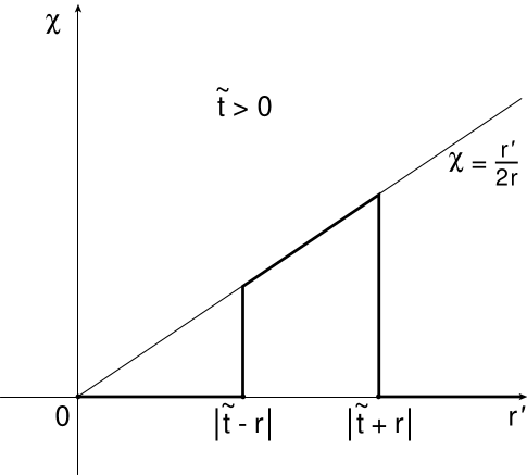
Figure 1: The function $\chi(r^{\prime})$ for $\tilde{t}>0$.

With (A.9), (A.10), or easier from Figure 1, we can calculate $\eta(\tilde{t},r,t^{\prime})$ defined in Eq. (4.9). First notice that for $\tilde{t}<0\ ,\ \eta=0$ and for $\tilde{t}>0\ ,\break\ \eta(r^{\prime}_{s}<|\tilde{t}-r|)=0$. The function is not equal to zero and assumes different values in two different intervals of values for $r^{\prime}_{s}$: for

$$|\tilde{t}-r|<r^{\prime}_{s}<|\tilde{t}+r|\,,\quad\tilde{t}>0\,,\qquad\quad\eta={1\over 4r}\ [r^{\prime 2}_{s}-(\tilde{t}-r)^{2}]\ ,$$

and for

$$r^{\prime}_{s}>|\tilde{t}+r|\,,\quad\tilde{t}>0\,,\qquad\quad\eta=\tilde{t}\ .$$

We thus find that ${\partial\eta\over\partial r}$ is only different from zero if $|\tilde{t}-r|\leq r^{\prime}_{s}\leq|\tilde{t}+r|$ and $\tilde{t}>0$:

$$\tilde{t}>0\ ,\ |\tilde{t}-r|<r^{\prime}_{s}<\tilde{t}+r\qquad{\partial\eta\over\partial r}={1\over 4r^{2}}\,(\tilde{t}^{2}-r^{2}-r^{\prime 2}_{s})\ .$$

Remembering that $\tilde{t}=\overline{t}-t^{\prime}$, we deduce from (A.13) the intervals of $t^{\prime}$ within which ${\partial\eta\over\partial r}\neq 0$:

$${\partial\eta\over\partial r}\neq 0\left\{{{\rm inside}\ \ \ \ r<r_{s}(t^{\prime})\ \ {\rm for}\ \ \overline{t}-(r^{\prime}_{s}+r)\leq t^{\prime}\leq\overline{t}-(r^{\prime}_{s}-r)\atop{\rm outside}\ \ r>r_{s}(t^{\prime})\ \ {\rm for}\ \ \overline{t}-(r^{\prime}_{s}+r)\leq t^{\prime}\leq\overline{t}-(r-r^{\prime}_{s})}\right.\ .$$

With (A.14) and ${\partial\eta\over\partial r}$ given in (A.13), we can calculate ${\bf A}$ given in (4.21). The lower bound of $t^{\prime}$ inside and outside of the shell is the same; it is a retarded time which we denote by $\overline{t}^{-}$,

$$\overline{t}^{-}=\overline{t}-r-r_{s}(\overline{t}^{-})\qquad r<r_{s}(\overline{t}^{-})\ .$$

There are, however, two different upper bounds $\overline{t}_{{\rm up}}$ which are both advanced times. Inside the shell,

$$\overline{t}_{{\rm up}}=\overline{t}^{+}=\overline{t}+r-r_{s}(\overline{t}^{+})\ ,\qquad r<r_{s}(\overline{t}^{+})\ .$$

Outside,

$$\overline{t}_{{\rm up}}=\overline{t}^{*}=\overline{t}-r+r_{s}(\overline{t}^{*})\ ,\qquad r>r_{s}(\overline{t}^{*})\ .$$

The vector potential ${\bf A}$ as given in (4.21) contains $\mbox{\boldmath$\nabla$}\eta={\partial\eta\over\partial r}{\hat{\bf r}}$. We replace ${\partial\eta\over\partial r}$ by its expression (A.13) and obtain

$${\bf A}=-{Q\over 4r^{3}}\int^{\overline{t}_{{\rm up}}}_{{\overline{t}}^{-}}{1\over r^{\prime}_{s}}{\overline{\mbox{\boldmath$\Omega$}}}^{\prime}_{\tau}\times{\bf r}\;[(\overline{t}-t^{\prime})^{2}-r^{2}-r^{\prime 2}_{s}]\;dt^{\prime}\ .$$

(b) The electromagnetic fields near the center

The scalar potential within the shell is a constant $A_{0}=-Q/r_{s0}$. As a result, both ${\bf E}$ and ${\bf B}$ are determined by ${\bf A}$. We shall here expand the expression of ${\bf A}$ near the center of the shell in powers of $x^{k}$. In this way we shall clearly see that ${\bf E},{\bf B}$ are not uniform, their dependence on $\overline{t}$ is entirely through the motions of the shell which we may specify how we like. To make the expansion we first rewrite (A.18) in the form

$${\bf A}={Q\over 4r^{3}}{\mbox{\boldmath$\psi$}}\times{\bf r}\ .$$

Thus, inside,

$${\overline{\mbox{\boldmath$\psi$ }}}=-\int^{t^{+}}_{t^{-}}{{\overline{\mbox{\boldmath$\Omega$}}}^{\prime}_{\tau}\over r^{\prime}_{s}}\;[(\overline{t}-t^{\prime})^{2}-r^{2}-r^{\prime 2}_{s}]\;dt^{\prime}\ .$$

Eqs. (A.19) and (A.20) are the equations quoted in (2.26) and (2.27).

To expand $\psi$ in powers of ${\bf r}$ we shall have to calculate the derivatives of $t^{+}$ and $t^{-}$ with respect to $t$. These are readily obtained from (A.15) and (A.16) in terms of the radial velocity of the shell

$$\overline{V}={dr_{s}\over d\overline{t}}\ ,$$

calculated at $\overline{t}^{+}$ and $\overline{t}^{-}$; thus,

$${d\overline{t}^{+}\over dr}={1\over 1+\overline{V}^{+}}\ \ ,\ \ {d\overline{t}^{-}\over dr}=-{1\over 1+\overline{V}^{-}}\ ,$$

where $\overline{V}^{+}=\overline{V}(\overline{t}^{+})$ and $\overline{V}^{-}=\overline{V}(\overline{t}^{-})$. The first derivative of $\psi$ with respect to $r$ is obtained with the help of (A.22) and is of the form

$${d{\mbox{\boldmath$\psi$}}\over dr}=2r{\mbox{\boldmath$\nu$}}\ ,$$

with

$${\mbox{\boldmath$\nu$}}={{\overline{\mbox{\boldmath$\Omega$}}}^{+}_{\tau}\over 1+\overline{V}^{+}}-{{\overline{\mbox{\boldmath$\Omega$}}}^{-}_{\tau}\over 1+\overline{V}^{-}}+\int^{\overline{t}^{+}}_{\overline{t}^{-}}{{\overline{\mbox{\boldmath$\Omega$}}}^{\prime}_{\tau}\over r^{\prime}_{s}}dt^{\prime}\ .$$

The method for deriving successive derivatives is obtained by calculating $\nabla^{2}(r^{2}{\bf A})$. One easily can find the following identity from (A.20) and (A.21)

$$-{2\over Q}\left[6{\bf A}+4({\bf r}\cdot{\mbox{\boldmath$\nabla$}}){\bf A}+r^{2}\,\nabla^{2}\,{\bf A}\right]={{\bf r}\over r}\times\left(3{\mbox{\boldmath$\nu$}}-{{\mbox{\boldmath$\psi$}}\over r^{2}}+r{d{\mbox{\boldmath$\nu$}}\over dr}\right)\ .$$

To expand ${\bf A}$ in powers of ${\bf r}$, we need the patience to calculate higher order derivatives of (A.25) and evaluate each of them at ${\bf r}=0$. The result to order 3 is as follows:

$${\bf A}={Q\over 6}\ \left[\left({d{\mbox{\boldmath$\nu$}}\over dr}\right)_{r=0}+\left({d^{3}{\mbox{\boldmath$\nu$}}\over dr^{3}}\right)_{r=0}{r^{2}\over 10}\right]\times{\bf r}+{\bf 0}(r^{5})\ .$$

The ${\bf E}$ and ${\bf B}$ fields are both $t$ and ${\bf r}$ dependent. To lowest order, ${\bf E}$ and ${\bf B}$ near the center are given by

$${\bf B}\simeq({\mbox{\boldmath$\nabla$}}\times{\bf A})_{r=0}={Q\over 3}\left({d{\mbox{\boldmath$\nu$}}\over dr}\right)_{r=0}\,={\bf B}_{c}\ ,$$

and

$${\bf E}\simeq-{1\over 2}\;{d{\bf B}\over dt}\times{\bf r}\ .$$

The magnetic field ${\bf B}_{c}=B_{c}{\hat{\bf z}}$ can be calculated from (A.24),

$$B_{c}={2Q\over 3}\;\left[{1\over 1+\overline{V}}\;{d\over d\overline{t}}\left({{\overline{\Omega}}_{\tau}\over 1+\overline{V}}\right)+{{\overline{\Omega}}_{\tau}/r_{s}\over(1+\overline{V})^{2}}\right]_{\overline{t}_{{\rm ret}}}\ ,$$

${\overline{t}}_{{\rm ret}}$ is the time at which the shell had a radius $r_{s}(\overline{t}_{{\rm ret}})$:

$$\overline{t}-r_{s{\rm ret}}=\overline{t}_{{\rm ret}}\ .$$

For a shell of constant radius $r_{s0}$ and rotating at constant angular velocity $\Omega_{0}$, $B_{c}=B_{0}$ given in (4.7).

Equation (A.29) with ${\overline{\Omega}}_{\tau}$ expressed in terms of ${\overline{\Omega}}$, see (4.3), is equation (2.33) when ${\overline{\Omega}}^{2}$ terms are neglected.

References

• [1] Barbour J. and Pfister H. eds. 1995 “Mach’s Principle: From Newton’s Bucket to Quantum Gravity” Einstein Studies, Volume 6 (Birkhäuser Boston)
• [2] Bičák J. 1979 Czech. J. Phys. B 29 945
• [3] Bičák J. and Dvořák L. 1980 Phys. Rev. D. 22 2933
• [4] Brill D.R. and Cohen J.M. 1966 Phys. Rev. 143 1011
• [5] Ciufolini I. and Wheeler J.A. 1995 Gravitation and Inertia (Princeton University Press, Princeton)
• [6] Goldwirth D. and Katz J. 1995 Class. Quant. Grav. 12 769
• [7] Israel W. 1966 Nuovo Cimiento B 44 1; Errata: 1967 Nuovo Cimiento B 48 463
• [8] Klein C. 1994 Class. Quant. Grav. 11 1539
• [9] Lindblom L. and Brill D. 1974 Phys. Rev. D. 10 3151
• [10] Lynden-Bell D., Katz J. and Bičák J. 1995 Mon. Not. R. Astr. Soc. 272 150; Erratum: 1995 Mon. Not. R. Astr. Soc. 277 1600
• [11] Lynden-Bell D. and Nouri-Zonoz M. 1998 Revs. Mod. Phys. 70 Vol. 2 427
• [12] Misner C., Thorne K.S. and Wheeler J.A. 1973 Gravitation (Freeman, San Francisco)
• [13] Møller C. 1972 The Theory of Relativity (Oxford University Press, Oxford)
• [14] Pfister H. and Braun K.H. 1985 Class. Quant. Grav. 2 909 and 3 335
• [15] Rindler W. 1997 Phys. Lett. A 233 25
• [16] Thirring H. 1918 Phys. Zeits. 19 33; Errata: 1921 Phys. Zeits. 22 29
• [17] Zel’manov A.L. 1956 Doklad. Acad. Sci. USSR 107 815