Doppler-Zeeman mapping of magnetic CP stars: The case of the CP star HD 215441

The recently developed method of Doppler-Zeeman mapping of magnetic CP stars (Vasilchenko et al.,1996, hereafter referenced as V.S.K., and also the contribution to this volume) confirmed its efficiency and robustness not only for model tests but also in the case of a real star.

The method was used for mapping Babcock’s star HD 215441, wich has the strongest known magnetic field and resolved Zeeman components in the lines of its spectra (Khokhlova et al., 1997, hereafter referenced as K.V.S).

We used the spectra of the CP star HD 215441 kindly given to us by Prof. Landstreet and which he had obtained with the coudé-spectrograph of the 3.5m Canada-France-Hawaii telescope and a Reticon detector. The spectral resolution was 0.1 Å  and the signal-to-noise ratio $S/N\geq 200$. We did not have polarization data at our disposal, but completely resolved $\pi$ and $\sigma$ components are practically equivalent to measured Stokes V parameter (except for the sign of the polarization and hence the lack of possibility to determine the sign of the magnetic-dipole vector). We assumed the signs of poles obtained in previous studies of this star (Landstreet et al., 1989).

Abundance maps for Si, Ti, Cr and Fe obtained from different lines of each element coincide very well. The magnetic field configurations obtained from 8 lines of four different elements were identical. They have been reliably determined for the star’s surface facing the observer. The maps are shown in Fig.1.

The magnetic field configuration is well fitted by a shifted-dipole model with dipole parameters $H_{D}=(21.3\pm 1.9)$ kG and shift $a=(0.12\pm 0.024)R^{*}$. The positive polar field $H_{p^{+}}=+(39.0\pm 2.0)$ kG and the negative $H_{p^{-}}=-(44.0\pm 9.0)$ kG. The local magnetic vectors were calculated for each point of the stellar surface. The position of maximum surface magnetic field $H_{S}$ on the visible hemisphere is determined to be $L=(5^{\circ}.6\pm 6^{\circ}.8)$, $\varphi=(63^{\circ}\pm 7^{\circ}.8)$ and the strength of the visible magnetic pole is $max(H_{S})=(42.3\pm 2.9)$ kG.

A comparison of magnetic and chemical maps definitely shows that at the visible magnetic pole most elements are strongly (Si, Cr) or slightly (Ti) underabundant but Fe is strongly overabundant. A large-scale ring structure around the magnetic pole is clearly seen on abundance maps (Fig. 1). The complete ring with strong Si overabundance is situated at low magnetic latitudes but not exactly on the magnetic equator. A strongly overabundant spot of Ti and of Cr is located on the background of a less overabundant ring, which is at the same place as the strong Si (and faint Fe) ring. Its location is particular, being not only near the magnetic equator, but also on the rotational equator.

The possibility of such a detailed and reliable comparison between magnetic field structure and abundance maps for magnetic CP stars is demonstrated for the first time in this study. The mapping became possible with a modest computer facility (PC Pentium) thanks to the method we used: analytic approximation of local line profiles and series expansion of the second order of multipole magnetic field geometry. The magnetic field of this star could be well approximated by a shifted dipole as well as by centered dipole and quadrupole.

We had to assume that the atmospheric model parameters $T_{\rm eff}$ and $\log g$ are constant over the surface of the star but this may not be true in reality. Due to evidently strong chemical inhomogeneities seen in Fig. 1, one may expect different metallicities at different places. But it is well known, that Kurucz’s models with different metallicities may provide big differences in computed line intensities. For our case it is demonstrated by Fig. 4 of K.V.S..

We cannot tell as yet, which element’s abnormal abundance is most efficient to produce such effects, because Kurucz’s metallicity is a scaled Solar abundance. One may only guess that C, N, O, Si, as most abundant elements, may play a dominant role as electron donors at the temperature of this star ($T_{\rm eff}=16000$) K, and also Fe, which is abundant and has many lines to contribute to the backwarming effect.

In general, the strict approach to solve the inverse problem of Doppler-Zeeman mapping requires iterations to be built as follows:

At each step of minimization of residual Functional, one uses the values of local abundances, local atmosphere models and local magnetic field vectors all obtained at the preceding step, and then performs the integration of the transfer equation to compute local Stokes profiles and local surface brightness, integrates them over the visible surface to calculate the ”observed” profile and the residual Functional for the next step of minimization. Obtaining the new set of local abundances, one should make computations of new local atmosphere models. Now the “loop” is closed and a new iteration may be started.

Keeping in mind that a dense coordinate grid on the stellar surface is desirable and that local abundances of more than one element are needed to be determined to make corrections to local atmosphere models at each iteration, the amount of time required for the strict solution by the above scheme is huge and unrealistic with the methods known and the available computers at the present time.

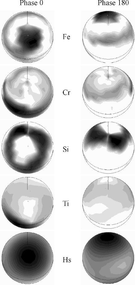
Figure1.: Chemical maps for Fe, Cr, Si and Ti and map of distribution of the local surface field $H_{S}$ on HD 215441 at phase $0^{\circ}$ (left column) and $180^{\circ}$ (right column)

The way we compute local Stokes profiles as a corrected analytic solution of transfer equations (as is described in detail in V.S.K) opens the possibility to solve the problem in a realistic time without serious loss of precision. It seems that one may not blame this method of local profiles computing for having not enough precision, until the problem of determining correct local atmosphere models is solved. It is impossible to guarantee better local profiles by strict numerical integration of the transfer equation only, without solving this problem. We have also to mention the problem of vertical stratification of abundances in CP stars, predicted by theoreticians (Babel & Mishaud, 1991) and investigated by observers (Babel, 1994; Romanyuk et al., 1992, and other attempts). If this stratification exists, further complications appear.

Returning to Fig. 1, one may see that Fe is overabundant near the magnetic pole. If a “metallicity” effect is determined by iron abundance, the iron spot must be hotter and there must be a bright spot there. Indeed, it is known that the maximum of the almost sinusoidal lightcurve of HD 215441 occurs at zero phase.

One may expect that the local intensity of Ti ii and Cr ii lines should decrease in a hot spot due to the second ionisation of these ions, and it is really the case, as Fig. 1 shows. But one cannot tell, whether this is the only reason, or whether real underabundances of Ti and Cr also exist.

For Si iii lines the temperature change has the reverse sign, their intensity should increase with increasing metallicity (increasing temperature in line-forming layers). But they decrease! This may be interpreted only as a real underabundance of Si near the magnetic pole.

A more detailed study of HD 215441 from spectra covering a wider wavelength range, involving more lines and other elements and also including polarization spectra, is urgently needed and seems to be very promising.

Acknowledgements. We thank Prof. J. Landstreet for giving us his reticon spectra of HD 215441. This work has been supported in part by the Soros International Science Foundation and the Government of the Russian Federation (grants nos. N2L000 and N2L300) and by the program “Astronomy” (project no 3-292).

References

- 1
- 2 Babel, J., Michaud, G.: Astron. Astrophys., 1991247, 155
- 3 Babel, J.: Astron. Astrophys., 1994283, 189
- 4 Khokhlova, V.L., Vasil’chenko, D.V., Stepanov, V.V., Tsymbal, V.V.: 1997, Astronomy letters23, 465
- 5 Kurucz, R.L.: 1992, Revista Mexicana de Astronomia y Astrofisica23, 181
- 6 Landstreet, J.D., Barker, P.K., Bohlender, D.A., Jewison, M.S.: 1989, Astrophys. J.344, 876
- 7 Romanyuk, I.I., Topil’skaya, G.P., Mikhnov, O.A.: 1992, inStellar magnetism,
- 8 Astronomy Letters22