Radiative transfer in Doppler Imaging

Abstract

The modern Doppler Imaging (DI) technique allows the reconstruction of different stellar surface structures based on accurate calculation of spectra of specific intensity. New applications like the mapping of the magnetic field vector put very stringent requirements on the radiative transfer (RT) solver which should be accurate, fast, and robust against numerical errors. We describe the evaluation of three different algorithms for our new magnetic DI code INVERS10. We also show the first results of numerical experiments made with the new code.

Key words: Stars: chemically peculiar – Stars: magnetic fields – Radiative transfer – Doppler Imaging

1 Introduction

Doppler Imaging is a method that allows to reconstruct the stellar surface structures from the rotational modulation of spectral line profiles (e.g. Piskunov & Rice 1993). DI is an iterative process. On each iteration the observational data (spectra taken at different rotational phases) are computed for the current surface distribution at each observed wavelength $\lambda$ and rotational phase $\phi$. This is done by integrating the specific intensity $I_{\lambda}(M)$ over the visible hemisphere. $I_{\lambda}(M)$ must be computed at each iteration for each $\lambda$, $\phi$, and surface element $M$ in a spectral range large enough to accommodate rotational Doppler shifts. Therefore, spectral synthesis of specific intensities is the most time consuming part of any DI algorithm!

With the improvement of computer performance and the expansion of the DI applications the need for a new RT became obvious as other solutions (e.g. tables of pre-computed local profiles) have been exhausted.

2 Magnetic RT solver

The goal of a magnetic DI code is to image the abundance (or temperature in case of late-type stars) together with the magnetic vector – 4 maps in total to be reconstructed simultaneously.

Three algorithms for RT solver in the presence of magnetic field have been considered: Runge-Kutta, Feautrier and Diagonal Element Lambda Operator (DELO). All three methods have been suggested and implemented by several people and detailed descriptions can be found in Landi Degl’Innocenti (1976, Runge-Kutta), Auer et al. (1977, Feautrier), and Rees et al. (1989, DELO). We strongly recommend those papers to anybody who wants to find out specific details about or implement any of these algorithms. Below we give a short outline of the magnetic RT problem and we describe the relevant properties of each algorithm.

The magnetic RT problem is a first order system of ordinary differential equations:

$$\mu\frac{d{\bf I}}{dz}=-{\em K}{\bf I}+{\bf j},$$ (1)

where ${\bf I}=(I,Q,U,V)$ is the vector of Stokes parameters, $\mu$ is the limb angle, ${\bf K}$ is the total absorption matrix and ${\bf j}$ is the total emission vector:

$${\em K} = \left(\begin{array}[]{rrrr}{\em k}_{c}+{\em k}_{l}\cdot\phi_{I}&{\em k}_{l}\cdot\phi_{Q}&{\em k}_{l}\cdot\phi_{U}&{\em k}_{l}\cdot\phi_{V}\\ {\em k}_{l}\cdot\phi_{Q}&{\em k}_{c}+{\em k}_{l}\cdot\phi_{I}&{\em k}_{l}\cdot\psi_{V}&-{\em k}_{l}\cdot\psi_{U}\\ {\em k}_{l}\cdot\phi_{U}&-{\em k}_{l}\cdot\psi_{V}&{\em k}_{c}+{\em k}_{l}\cdot\phi_{I}&{\em k}_{l}\cdot\psi_{Q}\\ {\em k}_{l}\cdot\phi_{V}&{\em k}_{l}\cdot\psi_{U}&-{\em k}_{l}\cdot\psi_{Q}&{\em k}_{c}+{\em k}_{l}\cdot\phi_{I}\end{array}\right)$$ (6)

$${\bf j} = \left(\begin{array}[]{r}{\em k}_{c}\cdot S_{c}+{\em k}_{l}\cdot S_{l}\phi_{I}\\ {\em k}_{l}\cdot S_{l}\phi_{Q}\\ {\em k}_{l}\cdot S_{l}\phi_{U}\\ {\em k}_{l}\cdot S_{l}\phi_{V}\end{array}\right),$$ (11)

where ${\em k}_{c}$ and ${\em k}_{l}$ are the continuum and line opacity and $S_{c}$ and $S_{l}$ are the continuum and line source functions. Assuming no polarization in the continuum and LTE at the continuum formation depth, $S_{c}$ is equal to the Planck function $B_{\nu}$. We note for later use that the diagonal elements of the absorption matrix are dominant, which provides the basis for the DELO algorithm.

The Zeeman splitting depends on the strength of the magnetic field and the Landé factors of $\pi$- and $\sigma$-components. The amplitude of the Stokes parameters depends on the orientation angles of the magnetic vector (the angle $\gamma$ between the magnetic vector and the line of sight, and the position angle $\chi$) via the absorption coefficients $\phi$’s and anomalous dispersion coefficients $\psi$’s. $\psi$’s are responsible for magneto-optical effects. The relation of $\phi$’s and $\psi$’s to the line profiles of the Zeeman components is given by:

$$\phi_{I} = \frac{1}{2}\phi_{p}\sin^{2}\gamma+\frac{1}{4}(\phi_{r}+\phi_{b})(1+\cos^{2}\gamma)$$

$$\phi_{Q} = \frac{1}{2}[\phi_{p}-\frac{1}{2}(\phi_{r}+\phi_{b})]\sin^{2}\gamma\cos 2\chi$$

$$\phi_{U} = \frac{1}{2}[\phi_{p}-\frac{1}{2}(\phi_{r}+\phi_{b})]\sin^{2}\gamma\sin 2\chi$$

$$\phi_{V} = \frac{1}{2}(\phi_{r}-\phi_{b})]\cos\gamma$$ (12)

$$\psi_{Q} = \frac{1}{2}[\psi_{p}-\frac{1}{2}(\psi_{r}+\psi_{b})]\sin^{2}\gamma\cos 2\chi$$

$$\psi_{U} = \frac{1}{2}[\psi_{p}-\frac{1}{2}(\psi_{r}+\psi_{b})]\sin^{2}\gamma\sin 2\chi$$

$$\psi_{V} = \frac{1}{2}(\psi_{r}-\psi_{b})]\cos\gamma$$

where indices p, b, r stand for $\pi$-components and blue and red $\sigma$-components.

The wavelength dependence of $\phi_{p}$, $\phi_{b}$, and $\phi_{r}$ are given by the Voigt function $V(a,v)$ while $\psi_{p}$, $\psi_{b}$, and $\psi_{r}$ are proportional to the Faraday-Voigt function $F(a,v)$. Humlíček (1982) gives very fast and accurate complex approximation for $V(a,v)$ and $F(a,v)$. We have implemented it as FORTRAN and C routines and compared it to a number of other approximations. We found Humlíček’s approximation to be the best.

2.1 Runge-Kutta magnetic RT integrator

Runge-Kutta techniques for solving the radiative transfer equations (1) integrate the Stokes parameters from the bottom of the atmosphere where an initial condition is set. A detailed description of the algorithm and its computer implementation (the MALIP code) has been given by Landi Degl’Innocenti (1976). He also analyses the main problems of the techniques. The advantage of Runge-Kutta is that the accuracy of the integration is checked at every step, so one can set the required accuracy a priori. We would also like to point out that the RT equation is one of a few rare cases where the 6th order Runge-Kutta offers substantial advantage over the conventional 4th order scheme because the accuracy can be checked without refining the step size. The main disadvantage is that different parts of the right hand side have a different depth dependence, and in order to achieve high accuracy, the algorithm is forced to use very small steps even deep in the atmosphere. To summarize: the Runge-Kutta technique is accurate but slow. It is primarily useful as a reference for other methods.

Now we shall turn to finite differences integration techniques which are more promising in terms of speed.

2.2 Feautrier magnetic RT integrator

The Feautrier method for solving the RT equation operates by splitting the intensity into two beams directed oppositely. The resulting equation is a second order ODE with two boundary conditions (one at the bottom and one at the surface of the atmosphere). Since the finite difference approximation involves 3 adjacent points for each step the method has excellent convergence properties. Application of the Feautrier method to non-magnetic RT requires the solution of a system of linear equations that form a tri-diagonal matrix. Although the accuracy cannot be checked at each step and the properties of the residual errors are much more complex than in the case of Runge-Kutta, refining the depth grid generally leads to a fast convergence and an accurate result. The Feautrier method has been extended to handle magnetic RT by Auer et al. (1977). In that case the tri-diagonal matrix is replaced by a block tri-diagonal, where each block is a 4$\times$4 matrix. The equations can be solved by analogy with the non-magnetic case, but back-substitution requires lots of 4$\times$4 matrix inversions and multiplications. The net result is a significant accumulation of numerical errors. For the centers of Zeeman components where the Voigt function is maximal and the Faraday-Voigt function is close to zero the difference between diagonal and non-diagonal elements in the absorption matrix reaches several orders of magnitude and with all the inversions, multiplications, and subtractions this scheme is bound to be numerically unstable. The alternative is to treat the block tri-diagonal matrix as a band diagonal matrix. The band should include 15 diagonals in order to cover all the blocks. The resulting scheme is robust against numerical errors for the price of only 20 % degradation in speed. Comparison with Runge-Kutta shows that for the same conditions, the Feautrier RT solver is about 30 times faster if the required accuracy is 10^-3. That is not quite fast enough for MDI, as the typical disk integration procedure requires approximately 10³ surface elements and the magnetic RT equation must be solved for each of them at several rotational phases.

2.3 DELO magnetic RT solver

Twelve years after the formulation of magnetic Feautrier algorithm, Rees et al. (1989) proposed a lambda operator methods serving as a one–way magnetic RT integrator. It is based on the fact that the absorption matrix is dominated by its diagonal elements. The principle can be easily illustrated in the non-magnetic case, but the DELO method is most impressive when integrating Stokes parameters.

In the non-magnetic case we can write the formal solution of the RT equation connecting the intensities at optical depths $\tau_{k}$ and $\tau_{k+1}$:

$$I(\tau_{k})\ =\ I(\tau_{k+1})\cdot e^{\displaystyle(\tau_{k}-\tau_{k+1})}\ +\ \int_{\tau_{k}}^{\tau_{k+1}}e^{\displaystyle-(\tau-\tau_{k})}S(\tau)d\tau$$ (13)

where $S(\tau)$ is the source function. If we assume that the source function in our depth interval is linear in $\tau$ and can be expressed as $S(\tau)=[(\tau_{k+1}-\tau)S_{k}+(\tau-\tau_{k})S_{k+1}]/(\tau_{k+1}-\tau_{k})$, then the integration in equation (13) can be performed analytically and we obtain a recurrence relation of the type:

$$I(\tau_{k})\ =\ P_{k}\ +\ Q_{k}\cdot I(\tau_{k+1})$$ (14)

with a boundary condition at the bottom of the atmosphere.

Generalization to the magnetic case is straightforward. After we implemented this method, we found it to be free of numerical instabilities and about 6 times faster than the Feautrier method (both are a direct result of much fewer matrix inversions). On the down side, we found that the convergence properties of the DELO method are not as good as for Feautrier (not surprising as the latter is a second order finite difference method), and it takes a much finer grid (4 – 8 times smaller step-size) to reach an accuracy of about 10^-3, thereby compromising the integration speed. After extensive experiments, we noticed that an adaptive depth grid can remedy the problem. The convergence is determined by the validity of linear approximation to the source function as described earlier in this section. It is much more efficient to refine the grid in the places where the source function variation is far from linear rather then adding extra points everywhere in the grid. Once implemented, this techniques proved to a be a winner. It usually takes as little as 20 % of additional grid points to reach the accuracy of 10^-3. DELO with adaptive refinement of the depth grid is the fastest technique with good numerical stability and convergence properties.

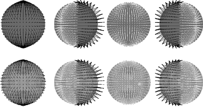
Figure1.: The reconstruction of a magnetic dipole (bottom row) using 4 Stokes parameters. The original field structure is shown in the top row.

3 The structure of INVERS10

With the new powerful magnetic RT solver based on the DELO method, we are able to compute local Stokes profiles “on the fly” rather than pre-calculating the interpolation tables. For each rotational phase, our new MDI code computes the specific intensity (Stokes) profiles for the local magnetic field and local chemical composition, and derivatives with respect to field components (radial, and the two tangential) and the abundance: $\partial{\bf I}/\partial B_{r}$, $\partial{\bf I}/\partial B_{m}$, $\partial{\bf I}/\partial B_{p}$, and $\partial{\bf I}/\partial X$. The disk integration of the flux profiles takes into account the rotational Doppler shifts and the radial-tangential macroturbulence. After disk integration the discrepancy and the regularization functions are computed together with the gradient vector. We use a modified conjugate gradient procedure to improve the solution. The modification makes use of the gradient vector during 1D optimization, since the gradient vector is computed with very little effort whenever the discrepancy function is evaluated. The overall procedure is efficient enough to reach a convergence for a typical size MDI problem (10 spectral lines, 100 wavelength points, 20 rotational phases) in 20-30 CPU hours on a fast workstation (an HP9000 C-180 in our case) with about 15 minutes per function evaluation.

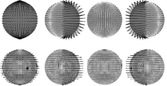
Figure2.: The reconstruction of a magnetic dipole (bottom row) using only 2 Stokes parameters ($I$ and $V$). The original field structure is shown in the top row.

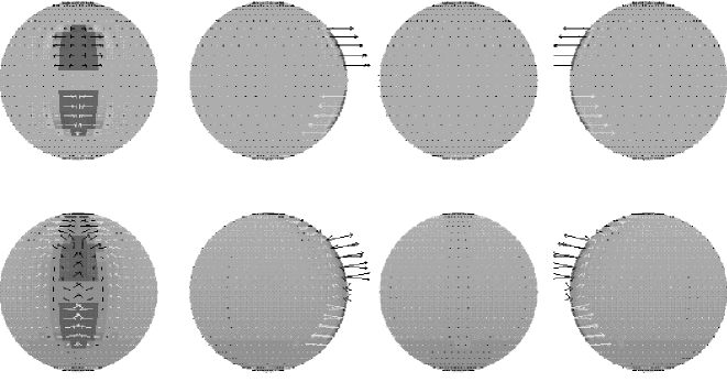
Figure3.: The reconstruction of 2 magnetic spots with enhanced iron abundance (bottom row) using 4 Stokes parameters. The original field/abundance structure is shown in the top row.

4 Numerical experiments

Numerical experiments offer the best way to assess the reliability of an inverse code. We start with an artificial star with known surface structure, compute a set of “observed” profiles, and then use them as input data for the inversion. Below we show the results of 3 such experiments with INVERS10. In all cases we have used a rather typical Fe ii 6141Å line, which has a Zeeman pattern with 6 $\pi$ and 10 $\sigma$ components. The effective Landé factor is 1.5. The “observed” profiles were computed for 20 equispaced rotational phases on a very fine surface grid using the Feautrier algorithm. The simulated profiles have been broadened by the instrumental profile corresponding to the resolving power of 80 000 and mixed with random noise corresponding to S/N of 300 for $I$ and 1000 for $Q$, $U$, and $V$. The $v\sin i$ of the star was set to 30km s^-1 with an inclination $i$ of 45^∘. Those parameters have been also used in the inversion. $\beta$ (in case of dipolar field) = 90^∘, abundance contrast is 2 dex.

In the first experiment (Fig. 1) we attempted to reconstruct the central dipolar field. The magnetic axis was tilted by 90^∘ from the rotational axis and the polar field was 8000 Gauss. Chemical composition was identical for every surface element. All four Stokes parameters were used in the inversion. The initial guess had the correct chemical composition but zero field. Figure1 shows the results of successful reconstruction. The cross-talk between magnetic field and abundance map of iron is less than 0.005 dex in the abundance map and less then 200G in the magnetic map.

In the next experiment (Fig. 2) we used the same test star, but only two Stokes parameters ($I$ and $V$) were used in the inversion. The result is shown in Figure2. The reconstructed magnetic field differs significantly from dipolar (most of the field vectors are directed along lines of constant latitudes in stellar coordinates, lower panel on Fig.2) while the cross-talk reached the level of 0.5 dex in the abundance map.

In the last experiment (Fig. 3) two small spots of high (+2 dex) iron abundance were located at zero longitude with symmetrical placement relative to the equator. Both spots have a radial magnetic field of 4000 Gauss, but opposite polarity. The results, shown in Figure3, demonstrate that 4 Stokes parameters, even with very modest phase coverage (as the spots are visible only in 10 phases), can be used to recover realistic field and chemical spot structures.

5 Conclusions

Although many more experiments will be required to investigate all the properties of the new code, even now it is clear that we can reliably reconstruct the vector magnetic field and that the observations of all four Stokes parameters are required. It is also clear that the MDI problem must be solved in a consistent way rather then by separately imaging magnetic field and abundance (or temperature), since (at least with incomplete observations) one of the variables can successfully mimic the other.

References

- 1 Auer, L.H., Heasley, J.N., House, L.L.: 1977, Astrophys. J.216, 531
- 2 Humlíček, J.: 1982, JQSRT27, 437
- 3 Landi Degl’Innocenti, E.: 1976, Astron. Astrophys., Suppl. Ser.25, 379
- 4 Piskunov, N., Rice, J.B.: 1993, Publ. Astron. Soc. Pac.105, 1415
- 5 Rees, D.E., Murphy, G.A., Durrant, C.J.: 1989, Astrophys. J.339, 1093