Turbulence as an Organizing Agent in the ISM

Abstract

We discuss HD and MHD compressible turbulence as a cloud-forming and cloud-structuring mechanism in the ISM. Results from a numerical model of the turbulent ISM at large scales suggest that the phase-like appearance of the medium, the typical values of the densities and magnetic field strengths in the intercloud medium, as well as the velocity dispersion-size scaling relation in clouds may be understood as consequences of the interstellar turbulence. However, the density-size relation appears to only hold for the densest clouds, suggesting that low-column density clouds, which are hardest to observe, are turbulent transients. We then explore some properties of highly compressible polytropic turbulence, in one and several dimensions, applicable to molecular cloud scales. At low values of the polytropic index $\gamma$, turbulence may induce the gravitational collapse of otherwise linearly stable clouds, except if they are magnetically subcritical. The nature of the density fluctuations in the high Mach-number limit depends on $\gamma$, and in no case resembles that resulting from Burgers turbulence. In the isothermal ($\gamma=1$) case, the dispersion of $\ln(\rho)$ scales like the turbulent Mach number. The latter case is singular with a lognormal density pdf, while power-law tails develop at high (resp. low) densities for $\gamma<1$ (resp. $\gamma>1$).

1 Introduction

One of the main features of turbulence is its multi-scale nature (e.g., [Scalo 1987]; [Lesieur 1990]). In particular, in the interstellar medium (ISM), relevant scale sizes span nearly 5 orders of magnitude, from the size of the largest complexes or “superclouds” ($\sim 1$ kpc) to that of dense cores in molecular clouds (a few $\times 0.01$ pc), with densities respectively ranging from $\sim 0.1$ cm^-3 to $\lower 2.15277pt\hbox{$\;\buildrel>\over{\sim}\;$}10^{6}$ cm^-3. Moreover, in the diffuse gas itself, even smaller scales, down to sizes several $\times 10^{2}$ km are active (see the chapters by Spangler and Cordes), although at small densities. Therefore, in a unified turbulent picture of the ISM, it is natural to expect that turbulence can intervene in the process of cloud formation ([Hunter 1979]; [Hunter & Fleck 1982]; [Elmegreen 1993]; Vázquez-Semadeni, Passot & Pouquet 1995, 1996) through modes larger than the clouds themselves, as well as in providing cloud support and determining the cloud properties, through modes smaller than the clouds ([Chandrasekhar 1951]; [Bonazzola et al. 1987]; [Léorat et al. 1990]; [Vázquez-Semadeni & Gazol 1995]). Moreover, another essential feature of turbulence is that all these scales interact nonlinearly, so that coupling is expected to exist between the large-scale cloud-forming modes and the small-scale cloud properties.

In this chapter we adopt the above viewpoint as a framework for presenting some of the most relevant results we have learned from two-dimensional (2D) numerical simulations of the turbulent ISM in a unified and coherent fashion, as it relates to the problems of cloud formation, the phase-like structure of the ISM and the topology of the magnetic and density fields, as well as internal cloud properties, such as their virialization and scaling relations (§ 2). Next we discuss recent results from multi-dimensional simulations and a simple heuristic model of one-dimensional polytropic turbulence, as a first attempt to gain more physical insight into the mechanisms responsible for the generation of the statistics of the density fluctuations in compressible turbulence (§ 3). Finally, we present a summary and conclusions in § 4.

2 Cloud Formation and Properties in the Turbulent ISM

In a series of recent papers (Vázquez-Semadeni et al. 1995 (Paper I), 1996 (Paper III); Passot, Vázquez-Semadeni & Pouquet 1995 (Paper II)), we have presented two-dimensional (2D) numerical simulations of turbulence in the ISM on the Galactic plane, including self-gravity, magnetic fields, simple parametrizations of standard cooling functions ([Dalgarno & McCray 1972]; [Raymond, Cox & Smith 1976]) as given by [Chiang & Bregman (1988)], diffuse heating mimicking that of background UV radiation and cosmic rays, rotation, and a simple prescription for star formation (SF) which represents massive-star ionization heating by turning on a local source of heat wherever the density exceeds a threshold $\rho_{\rm t}$. Supernovae are now being included (Gazol-Patiño & Passot 1998; see also Korpi, this Conference, for analogous simulations in 3D). The simulations follow the evolution of a 1 kpc² region of the ISM at the solar Galactocentric distance over $\sim 10^{8}$ yr and are started with Gaussian fluctuations with random phases in all variables. The initial fluctuations in the velocity field produce shocks which trigger star formation which, in turn, feeds back on the turbulence, and a self-sustaining cycle is maintained. These simulations have been able to reproduce a number of important properties of the ISM, suggesting that the processes included are indeed relevant in the actual ISM. Some interesting predictions have also resulted.

2.1 Effective Polytropic Behavior and Phase-Like Structure

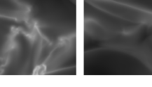
Figure 1: Two views of the density field in a simulation of 1 kpc² of the ISM on the Galactic plane, one at a) $t=6.37\times 10^{7}$ yr (left), the other at b) $t=7.80\times 10^{7}$ yr (right). The large-scale structures are contracting gravitationally, while the smaller structures within them change significantly due to the turbulent motions.

One of the earliest results of the simulations is a consequence of the rapid thermal rates ([Spitzer & Savedoff 1950]), faster than the dynamical timescales by factors of 10–$10^{4}$ in the simulations (Paper I). Thus, the gas is essentially always in thermal equilibrium, except in star-forming regions, and an effective polytropic exponent $\gamma_{\rm e}$ ([Elmegreen 1991]) can be calculated, which results from the condition of equilibrium between cooling and diffuse heating, giving an effectively polytropic behavior $P_{\rm eq}\propto\rho^{\gamma_{\rm e}}$, where $\rho$ is the gas density (see Papers II and III for details). Even though the heating and cooling functions used do not give a thermally unstable (e.g., [Field, Goldsmith & Habing 1969]; [Balbus 1995]) regime at the temperatures reached by the simulations, they manage to produce values of $\gamma_{\rm e}$ smaller than unity for temperatures in the range 100 K $<T<10^{5}$ K, implying that denser regions are cooler. Upon the production of turbulent density fluctuations, the flow reaches a temperature distribution similar to that resulting from isobaric thermal instabilities ([Field, Goldsmith & Habing 1969]), but without the need for them. Note, however, that in this case there are no sharp phase transitions.

2.2 Cloud Formation

In the simulations, the largest cloud complexes (several hundred pc) form simply by gravitational instability. Although in Paper I it was reported that no gravitationally bound structures were formed, this conclusion did not take into account the effective reduction of the Jeans length due to the small $\gamma_{\rm e}$ of the fluid. Once this effect is considered, it is found that the largest scales in the simulations are unstable. This process is illustrated in fig. 1, which shows two snapshots of the logarithm of the density in a simulation at a resolution of 512 grid points per dimension (run 28 from Paper II), one at $t=6.37\times 10^{7}$ yr (a), with minimum and maximum densities of 0.04 and 36.1 cm^-3, and the other at $t=7.80\times 10^{7}$ yr, with extrema of 0.046 and 58 cm^-3. The two very large scale structures in the upper and lower halves of the integration box, are seen to have contracted at the later time, and the voids have expanded. Nevertheless, inside such large-scale clouds, an extrememly complicated morphology is seen in the higher-density material, as a consequence of the turbulence generated by the star formation activity. The medium- and small-scale clouds are thus turbulent density fluctuations.

2.3 Cloud and magnetic field topology

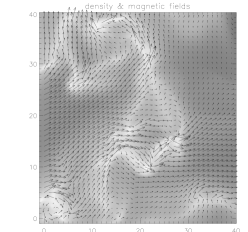
Figure 2: Gray-scale image of the logarithm of the density field, with superimposed magnetic field vectors. Shown is a subfield of $200\times 200$ pc ($160\times 160$ pixels), from a simulation at resolution of 800 grid points per dimension (VBR97). The minimum and maximum magnetic field intensities are 0.13 and 26.6 $\mu$G, respectively. The axes show arbitrary units. See text for feature description.

The topology of the clouds formed as turbulent fluctuations in the simulations is extrememly filamentary. This property apparently persists in 3D simulations (see chapters by Ostriker, Stone, Mac Low and Padoan). Interestingly, the magnetic field also exhibits a morphology indicative of significant distortion by the turbulent motions (Paper II; [Ballesteros-Paredes & Vázquez-Semadeni 1998]). The field has a tendency to be aligned with density features, as shown in fig. 2. Even in the presence of a uniform mean field, motions along the latter amplify the perpendicular fluctuations due to flux freezing, while at the same time they produce density fluctuations elongated perpendicular to the direction of compression. This mechanism also causes many of the density features to contain magnetic field reversals (e.g., the feature near the lower left corner) and bendings (e.g., the feature down and to the right off the center, with coordinates $x\sim 25,y\sim 12$). It happens also that magnetic fields can traverse the clouds without much perturbation, as seen for example in the feature at $x=21,y=30$. These results are consistent with the observational result that the magnetic field does not seem to vary much along clouds ([Goodman et al. 1990]), and in general does not present a unique kind of alignment with the density features. On the other hand, recent observations have found field bendings similar to those described here (Crutcher, this volume). Also, field reversals in clouds have been recently observed ([Heiles 1997]).

It is important to note that the “pushing” of the turbulence on the magnetic field occurs for realistic values of the energy injection from stars and of the magnetic field strength, which ranges from $\sim 5\times 10^{-3}\mu$G (occurring at the low density intercloud medium) to a maximum of $\sim 25\mu$G, which occurs in one of the high density peaks, although with no unique $\rho$-$B$ correlation ([Paper II]). Observationally, larger values of the field occur only on much smaller scales than those resolved by our simulations (1.25 pc in at resolution of $800^{2}$ grid points) ([Heiles et al. 1993]). Thus, the simulations suggest that the effect of the magnetic field is not as strongly dominating as often assumed in the literature. This is also in agreement with the fact that the magnetic and kinetic energies in the simulations are in near global equipartition at all scales, as shown by their energy spectra (fig. 5 in [Paper II]).

Finally, note that the fact that the magnetic spectrum exhibits a clear self-similar (power-law) range, together with the fact that the fluctuating component of the field is in general comparable or larger than the uniform field, suggests strongly that the medium is in a state of fully developed MHD turbulence, rather than being a superposition of weakly nonlinear MHD waves.

2.4 Cloud scaling properties

An important question concerning the clouds formed in the simulations is whether they reproduce some well-known observational scaling and statistical properties of interstellar clouds, most notably the so-called Larson’s relations between velocity dispersion $\Delta v$, mean density $\rho$ and size $R$ ([Larson 1981]), and the cloud mass spectra (e.g., [Blitz 1991]). Vázquez-Semadeni, Ballesteros-Paredes & Rodríguez (1997, hereafter [VBR97]) have studied the scaling properties of the clouds in the simulations, finding that the cloud ensemble exhibits a relation $\Delta v\propto R^{0.4\pm 0.08}$ and a cloud mass spectrum $dN(M)/dM\propto M^{-1.44\pm 0.1}$, both being consistent with observational surveys, especially those specifically including gravitationally unbound objects (e.g., [Falgarone, Puget & Pérault 1992]). However, it was found that no density-size relation like that of Larson ($\rho\propto R^{-1}$) is satisfied by the clouds in the simulations. Instead, the clouds occupy a triangular region in a $\log\rho$–$\log R$ diagram, as shown in fig. 8 of [VBR97], with only its upper envelope being close to Larson’s relation. This implies the existence of clouds of very low column density, which are presumably turbulent transients, and can be easily missed by observational surveys if they do not integrate for long enough times. A few observational works, however, point towards the existence of transients ([Loren 1989]; [Magnani, La Rosa & Shore 1993]) and low-column density clouds, with masses much smaller than those estimated from virial equilibrium ([Falgarone, Puget & Pérault 1992]).

An implication of Larson’s relations is the so-called logatropic “equation of state” ([Lizano & Shu 1989]). [Vázquez-Semadeni, Cantó & Lizano (1998)] have investigated whether this behavior is verified in numerical simulations of gravitational collapse with initially turbulent conditions. A logatropic behavior would imply a scaling $\Delta v\propto\rho^{-1/2}$. However, a scaling $\Delta v\propto\rho^{\alpha}$, with $1/4<\alpha<1/2$ was observed, suggesting a polytropic behavior instead. This was interpreted as meaning that the logatropic equation of state was obtained by an invalid assumption, namely that Larson’s relations are applicable to a thermodynamic process on a cloud of fixed mass. Instead, they seem to represent only the conditions of a (possibly relaxed) ensemble of clouds of different masses, and so are inapplicable to the former case.

3 Results on polytropic compressible turbulence

3.1 Production and stability of turbulent density fluctuations

In view of the effective polytropic behavior exhibited by the simulations (§ 2.1), a natural abstraction is to consider the behavior of purely polytropic fluids, whose equation of state is $P=\rho^{\gamma_{\rm e}}/\gamma_{\rm e}$. For such a fluid, it has been shown in ([Paper III]) that the density jump $X\equiv\rho_{2}/\rho_{1}$ in a shock in a polytropic gas satisfies

$$X^{1+\gamma_{\rm e}}-(1+\gamma_{\rm e}M^{2})X+\gamma_{\rm e}M^{2}=0,$$ (3.1)

where $M$ is the Mach number upstream of the shock. From this equation, we recover the fact that the compression ratio for an isothermal shock ($\gamma_{\rm e}=1$) is $M^{2}$, but we also see that $X\rightarrow e^{M^{2}}$ as $\gamma_{\rm e}\rightarrow 0$, a density jump which can be much larger than the isothermal one.

Turbulence-induced fluctuations can either collapse or rebound, depending on their cooling and dissipating abilities (e.g., [Hunter & Fleck 1982]; [Hunter et al. 1986]; Elmegreen & Elmegreen 1978; Vishniac 1983, 1994; [Elmegreen 1993]). The critical value of $\gamma_{\rm e}$ for which a turbulent density fluctuation formed by an $n$-dimensional compression can collapse was given in [Paper III] as $\gamma_{\rm cr}\equiv 2(1-1/n)$. The same criterion was given by [McKee et al. (1993)] for fixed $\gamma_{\rm e}\sim 1$ as an indication that 1-dimensional shock compressions cannot cause collapse. Instead, we can argue that the combination of small enough $\gamma_{\rm e}$ and compressions in more than one dimension (shock collisions) can trigger collapse. [Scalo et al. (1998)] have recently discussed the possible values of $\gamma_{\rm e}$ in the cold ISM, finding that, although with large uncertainty, $\gamma_{\rm e}\sim 1/3$ is possible at densities $\lower 2.15277pt\hbox{$\;\buildrel>\over{\sim}\;$}5\times 10^{4}$ cm^-3, thus making the collapse of shock-compressed cores feasible.

3.2 Statistics of density fluctuations in polytropic turbulence

The turbulent formation of clouds in the ISM must ultimately be described by the statistics of density fluctuation production in compressible turbulence. Therefore, it is of interest to investigate the probability density function (pdf) of the density fluctuations that develops in numerical simulations. Interestingly, the pdfs reported for a variety of flows show important qualitative differences. [Porter, Pouquet & Woodward (1991)] reported an exponential pdf for 3D, weakly compressible thermodynamic turbulence. Power-law pdfs have been reported for low-Reynolds number, one-dimensional Burgers flows ([Gotoh & Kraichnan 1993]) and for the simulations described in § 2, as well as for two-dimensional Burgers flows (Scalo et al. 1998), while lognormal pdfs have been reported for isothermal 2D ([Vázquez-Semadeni 1994]) and 3D ([Padoan, Nordlund & Jones 1997]) simulations.

Passot & Vázquez-Semadeni (1998, hereafter [PVS98]) have investigated the simplest case of a one-dimensional purely hydrodynamic flow by means of a heuristic model and very high resolution (up to 6144 grid points) numerical simulations. Here, we summarize these results briefly. In order to study the production of the local density fluctuations, it is convenient to describe them as a sequence of isolated, discrete jumps ([Vázquez-Semadeni 1994]). Consider first the isothermal ($\gamma_{\rm e}=1$) case, whose governing equations read

$$\frac{Du}{Dt}=-\frac{1}{M^{2}}\frac{\partial}{\partial x}s$$ (3.2)

$$\frac{Ds}{Dt}=-\frac{\partial}{\partial x}u,$$ (3.3)

where $\rho$ is the fluid density, $u$ is the velocity, $s=\ln\rho$ and $M$ is the Mach number of the velocity unit. Note that these equations are invariant upon the change $s\rightarrow s+b$, where $b$ is an arbitrary constant, reflecting the fact that the sound speed does not depend on the density in this case. Consider now the sequence of density jumps $\rho_{2}/\rho_{1}$. This is a sequence of multiplicative steps, and, consequently, additive steps in $s=\ln\rho$. But, because of the translation invariance mentioned above, a jump of a given magnitude must have the same probability of occurrence, independently of the initial density. Thus, the sequence involves events with the same probability distribution, and by the Central Limit Theorem it must converge to a Gaussian distribution in $s$, or, equivalently, a lognormal distribution in $\rho$ (see Nordlund, this volume, for an alternative derivation), explaining the reported pdfs in the isothermal case.

Figure 3: Logarithm of the variance of a) $s\equiv\ln\rho$ (left) and b) the density $\rho$ (right) vs. the logarithm of the rms Mach number in one-dimensional simulations of polytropic turbulence. Note that $\sigma_{s}^{2}$ scales as $M_{\rm rms}^{2}$, while $\sigma_{\rho}^{2}$ increases faster than $M_{\rm rms}^{2}$.

In order to fully characterize the pdf, it is necessary to determine its mean and variance. Concerning the latter, [PVS98] have suggested, through an anlysis of the shock and expansion waves in the system, that for a large range of Mach numbers the typical size of the logarithmic jump is expected to be $\sigma_{s}\sim M_{\rm rms}$, where $M_{\rm rms}$ is the rms Mach number. This result is verified numerically, as shown in fig. 3a. Note that fig. 3b shows the scaling of the linear density variance $\sigma_{\rho}^{2}$ vs. $M_{\rm rms}^{2}$. An exponential behavior is observed, most noticeable at large Mach numbers, in agreement with the relation $\sigma_{s}^{2}=\ln(1+\sigma_{\rho}^{2})$ which holds for a lognormal distribution. This contrasts with recent claims that it is $\sigma_{\rho}$ which scales as $M_{\rm rms}$ ([Padoan, Nordlund & Jones 1997]; Nordlund, this volume). This discrepancy can be understood as a consequence of the similarity between the two variances at small Mach numbers, together with the fact that the simulations from which those authors reached their conclusion were three-dimensional, implying that a significant fraction of the kinetic energy was in rotational modes (reportedly $\sim 80$ %), and thus not available for producing density fluctuations. Instead, in the 1D simulations of [PVS98], all of the kinetic energy is compressible.

Concerning the mean $s_{0}$ of the distribution, it can be directly evaluated from the mass conservation condition $\langle\rho\rangle=\int_{-\infty}^{+\infty}e^{s}P(s)ds=1$, where $P(s)$ is the pdf of $s$, yielding $s_{0}=-\sigma_{s}^{2}/2$. With all this in mind, we can then write the model pdf for $s$ as

$$P(s)ds=\frac{1}{\sqrt{2\pi\sigma_{s}^{2}}}\exp\bigl{[}-\frac{(s-s_{o})^{2}}{2\sigma_{s}^{2}}\bigr{]}ds,$$ (3.4)

with $\sigma_{s}^{2}=\beta M_{\rm rms}^{2}$, and $\beta$ a proportionality constant. The numerical simulations confirm the dependence of the width and mean of the distribution with $M_{\rm rms}$ ([PVS98]).

We next consider the case $\gamma_{\rm e}\neq 1$. The governing equations can now be written as

$$\frac{Du}{Dt}=\frac{1}{(1-\gamma_{\rm e})M^{2}}\frac{\partial}{\partial x}e^{-v}$$ (3.5)

$$\frac{Dv}{Dt}=-(1-\gamma_{\rm e})\frac{\partial}{\partial x}u.$$ (3.6)

Interestingly, these equations return to the form of eqs. (3.2) and (3.3) upon the density-dependent rescaling $M\rightarrow M(s;\gamma_{\rm e})=Me^{(1-\gamma_{\rm e})s/2}$. Thus, we formulate the ansatz that the form of the pdf also remains the same, provided the above replacement is made. After relocating the term in $s_{0}$ from inside the exponential function to the normalization constant, we can write the model pdf as

$$P(s;\gamma_{\rm e})ds=C(\gamma_{\rm e})\exp\Bigl{[}\frac{-s^{2}e^{(\gamma_{\rm e}-1)s}}{2M^{2}}-\alpha(\gamma_{\rm e})s\Bigr{]}ds.$$ (3.7)

Figure 4: Density pdfs for two 1D simulations of polytropic turbulence, one with $\gamma_{\rm e}=0.3$ (left), and the other with $\gamma_{\rm e}=1.7$ (right), both with $M=3$.

Note that this is a particular form of the pdf valid only in a range of $s$-values ([PVS98]), but for illustrative purposes it suffices here. This equation shows that when $(\gamma_{\rm e}-1)s<0$, the pdf asymptotically approaches a power law, while in the opposite case it decays faster than a lognormal. Thus, for $0<\gamma_{\rm e}<1$, the pdf approaches a power law at large densities ($s>0$), and at low densities for $\gamma_{\rm e}>1$. The former case is in agreement with the pdfs reported for our 2D simulations, which in general have $\gamma_{\rm e}<1$. The 1D simulations also verify this result for $\gamma_{\rm e}>1$ (fig. 4). See Nordlund (this volume) for a parallel treatment of this problem.

It is important to note that even at very small values of $\gamma_{\rm e}$ ($\sim 0.01$), the fast drop of the pdf at low densities is still observed, due to the factor $e^{(\gamma_{\rm e}-1)s}$ in the exponential in eq. 3.7, which in turn implies that there is always a range of $s$-values in which the pressure is not negligible in the hydrodynamic case, for any $\gamma_{\rm e}$. This leads to the speculation that the pdf for Burgers flows, which are strictly pressureless, should exhibit power laws at both large and small densities. This speculation is also verified numerically ([PVS98]). Thus, the Burgers case appears to be singular, not being the limit of hydrodynamic flows as $\gamma_{\rm e}\rightarrow 0$, at least as far as the pdf is concerned.

4 Conclusions

In this Chapter we have discussed a scenario in which turbulence plays a fundamental role in the production and determination of interstellar cloud properties. Large-scale turbulent modes intervene in the former, while small-scale modes seem to participate in determining cloud scaling relations. ISM features that appear naturally in our simulations are the phase-like appearance (a consequence of turbulent density fluctuation production together with an effective polytropic exponent $\gamma_{\rm e}<1$), density and magnetic field topologies and field strength ranges, and the velocity dispersion-size relation and cloud mass spectrum. However, the suggestions are made that the Larson (1981) density-size scaling relation may be an artifact of surveys which do not integrate for long enough times, and that the logatropic equation of state ([Lizano & Shu 1989]) is not verified in highly dynamic situations.

Given the possible nature of clouds as turbulent density fluctuations, their production in polytropic flows was also discussed. The density jump across shocks and a criterion for the collapse of these fluctuations were advanced. Finally, a model for the probability density function of the fluctuations was described, which satisfactorily explains the pdf shapes observed in isothermal, polytropic and Burgers cases. Future work in this area will address the fully thermodynamic and magnetic cases, aiming at explaining other forms of the pdf, which have been observed numerically, but not produced by the model.