Comparison of two different extinction laws with Hipparcos observations

Abstract

Interstellar absorption in the galactic plane is highly variable from one direction to another. In this paper colour excesses and distances from a new open cluster sample are used to investigate the spatial distribution of the interstellar extinction. An inverse method (Tarantola & Valette, 1982) is used to construct the extinction map in the galactic plane below $|b|<10^{o}$. The $A_{v}(r,l)$ diagrams are compared with those derived from individual stars (Arenou et al. 1992, Neckel & Klare 1980). An analytic expression for the interstellar extinction as a function of galactic longitude and distance in the solar neighborhood is given. The comparison of the model predictions with Hipparcos observations in the 4-dimensional space of ($V$, $B-V$, $H_{v}$, $r$) shows that our extinction model provides a better fit to the data. However, a new and more detailed extinction model is still lacking.

1 Introduction

The light extinction caused by the interstellar medium in the solar neighborhood alters the apparent brightness of the stars and thus their intrinsic properties (absolute magnitude, intrinsic colour, etc.). For this reason, it is crucial to know the effects of the interstellar medium on the radiation we receive from the stars, and to build models up which reasonably predict the amount of extinction in a given direction.

Bahcall & Soneira (1980) have used Sandage’s extinction law (1972) in their model of the Galaxy, and compared model predictions with star count observations in 17 fields. They found that, at $\mid$ b $\mid$ $>$ 10^o, the Sandage absorption law is a good approximation to observations. However, at low galactic latitudes, the absorptions are patchy and poorly known. In the context of our study on stellar kinematics from Hipparcos observations and open cluster (Chen et al, 1998), we need a reliable extinction model at low galactic latitudes.

Neckel & Klare (1980) derived extinctions and distances for more than 11000 stars and investigated the spatial distribution of the interstellar extinction at $\mid$ b $\mid$ $<$ 7.6^o. Their results are shown in a series of diagrams. Using a larger sample (about 17000 stars) with MK spectral types and photoelectric photometry, Arenou et al. (1992) (hereafter AGG92) constructed an extinction model in which the sky was divided into 199 cells. In each cell, a quadratic relation was adopted. This extinction model will be the reference in this paper. Hakkila et al. (1997) have developed a computerized model of large-scale visual interstellar extinction. The code merges several published studies (FitzGerald 1968; Neckel & Klare 1980; Berdnikov & Pavlovskaya 1991; AGG92; etc.), and can be used for making corrections to individual observations and for correcting statistical sample. With extinctions determined from Strömgren photometry and parallaxes from Hipparcos for a sample of 3799 stars, Vergely et al (1997) have constructed a three dimension distribution of absorbing matter in the solar neighbourhood. However, all these authors use similar dataset (stars along with their corresponding colors, magnitudes, and spectral/morphological classification types) so that the results are not statistically independent (Hakkila et al. 1997).

In this paper, we are going to use open clusters rather than individual stars to investigate the distribution of interstellar extinction, and compare our results with those found in the literature. The reason for this investigation is twofold. First, the advent of CCDs with their sensitivity and linearity has allowed to obtain deep photometry of open clusters (Carraro & Ortolani, 1994, Kaluzny 1994). Second, distances and reddening for open clusters are more reliable than those from individual stars, simply because one is dealing with a group of stars and therefore the results are less sensitive to individual errors. Thus the open clusters system provides us with another way to obtain informations on A_v as a function of the galactic longitude $l$ and distance $r$.

Pandey & Mahra (1987) firstly used the open cluster catalogue of Janes & Adler (1982) to investigate the spatial distribution of interstellar extinction within 2 kpc. Their results are presented in graphical form. No analytical expression for the interstellar extinction has been presented. In this paper, we have used a new open cluster database and an inverse method (Tarantola & Valette, 1982) to derive an analytical expression of the interstellar extinction in the solar vicinity, and compared different extinction models with Hipparcos observations. In section 2 we present the data used in this paper. In section 3 we briefly explain the AGG92’s model and compare it with our open cluster data. In section 4, we construct a new extinction model from open cluster system. In section 5 the predictions from AGG92’s extinction model and our extinction model are compared with the Hipparcos data. The main conclusions are summarized in section 6.

2 The Data

The main source of the data in this investigation is the Open Cluster Data Base (Mermilliod 1992). In this database, the reddening and distance for each cluster were determined from a system of weights corresponding to the precision of open cluster data. 412 open clusters with reddening and distance are listed in the database. In addition to this data, from the list of open clusters, we have checked each cluster which has no information about reddening and distance from ADS database to see whether there are new observations published after 1992. Finally, we have found 22 such clusters, mostly due to the observations from Padova and Boston group (Friel, 1995). Thus, the present study is based on the observed distances and colour excesses of 434 open clusters. The ratio of total to selective absorption, $R$=3.1, was adopted to obtain total absorption from selective absorption $E(B-V)$. In Figure 1 we show the distribution of the open clusters in the ($l$, $b$) plane of galactic longitude and galactic latitude. We can see that most open clusters (91%) lie on the galactic plane ( $\mid$ b $\mid$ $\leq$ 10^o ), and that the distribution of open clusters is not homogeneous in galactic longitude ($l$). In the direction between $l$= 30^o and $l$ = 90^o, and between $l$ = 145^o and $l$ = 220^o, fewer open clusters are found.

Figure 1: The distribution of the open clusters in the plane of galactic longitude and latitude

In Figure 2 we show the histogram of the distance $r$. In the Open Cluster Data Base (Mermilliod, 1992), the errors of the extinction and distance are not given. We suppose that the error $\sigma_{Av}$ can be written :

$$\sigma_{Av(obs)}=\Delta Av(obs)_{cal}+\Delta Av(obs)_{r}$$ (1)

Where $\Delta Av(obs)_{cal}$ is the calibration error approximately equal to 0.1 mag and $\Delta Av(obs)_{r}$ the extinction error due to the distance error. As a first approximation we consider that the distance determination and $Av(obs)$ are uncorrelated, and that the relative distance error is 0.25. Then, we have

$$\sigma_{Av(obs)}=0.1+0.25Av(obs)$$ (2)

Figure 2: Histogram of distance $r$ to the Sun of the open clusters

From Hipparcos parallaxes, Mermilliod et al (1997) and van Leeuwen & Hansen Ruiz (1997) claimed that the distance of young Pleiades cluster is 10$\sim$ 15% smaller than its photometric distance. In order to check whether a systematic bias exists on all determinations of open clusters from photometric methods, we have compared the open cluster distance derived from Hipparcos data (Robichon et al. 1997; Mermilliod et al. 1997) with those in Mermilliod’s catalogue. Figure 3 shows the distance derived from Hipparcos parallaxes ($r_{1}$) against those in Mermilliod’s open cluster database ($r_{2}$), no systematic trend has been found.

Figure 3: The open cluster distance derived from Hipparcos data ($r1$) against those in Mermilliod’s open cluster database ($r2$)

3 AGG92’s extinction model

AGG92 have used INCA database (Gómez et al. 1989; Turon et al. 1991) to construct a tridimensional model of the galactic interstellar extinction. For each star the distance $r$ to the sun and the visual extinction $A_{v}$ have been computed from MK spectral type and photoelectric colour index.

Figure 4: The observed extinction A_v(obs) against that derived from AGG92’s model A_v (model) for our open cluster sample

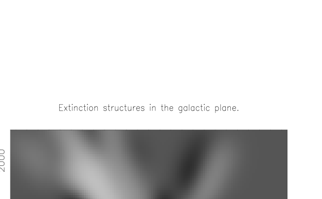
Figure 5: Extinction structures in the Galactic plane

The sky was divided in 199 cells. In each cell, based on the work of Neckel & Klare (1980), a quadratic relation was adopted:

$$A_{v}=\alpha r+\beta r{{}^{2}}$$ (3)

Figure 6: Extinction structures in the cross section of the galactic plane

Figure 7: Histogram of $\delta$ value ($\delta=\frac{Av(obs)-Av(model)}{\sigma_{Av(obs)}}$).

Figure 8: The extinction derived from our model Av(model) against the observed one Av(obs).

Figure 9: The extinction as a function of distance for each of the 36 cells. The solid lines are the results in this study from the inverse method, the dashed lines are the results from Arenou et al. (1992). The crosses (+) are the open cluster sample.

Figure 9: (continued)The extinction as a function of distance for each of the 36 cells. The solid lines are the results in this study from the inverse method, the dashed lines are the results from Arenou et al. (1992). The crosses (+) are the open cluster sample.

For each cell an analytic expression of the interstellar monochromatic extinction at V-magnitude A_v($r$,$l$,$b$) was obtained. We have used AGG92’s model to derive the extinction at the position of each open cluster in our sample. In Figure 4, we plot the observed extinction $A_{v}$(obs) against that derived from AGG92’s model $A_{v}$(model). It can be seen that AGG92’s model underestimates large extinction value. Since AGG92 used only stars brighter than V = 13 mag, as they stated, their model cannot be extrapolated farther than 1 kpc. From Figure 4 we have also found that AGG92’s results are higher than the observations for small distance ($r<500$ pc). AGG92 pointed out that a slight overestimation of $A_{v}$ for small distance is expected in their model, this is consistent with what we have noticed from our open cluster sample. In the following sections, we use open clusters with $\mid$ b $\mid$ $\leq$ 10^o to derive the interstellar extinction at low galactic latitudes and construct a new extinction model in solar neighbourhood.

4 Using open clusters to derive the interstellar extinction at low galactic latitudes

In order to determine the opacity in each point of the space in a circle of 2500 pc around the Sun, we utilized an inverse method (Tarantola & Valette, 1982; Valette & Vergely, in preparation) which for the first time has been applied to detect extinction structures in the Hipparcos data (Vergely et al., 1997).

Table 1: The coefficients of the extinction curves in different longitudes

Range of $l$	$a_{1}$	$a_{2}$	$a_{3}$	$a_{4}$
(degrees)	(mag.kpc-1)	(mag.kpc-2)	(mag.kpc-3)	(mag.kpc-4)
0-10	0.752	0.610	0.090	-0.387
10-20	0.500	3.012	-3.659	1.378
20-30	0.245	5.468	-7.721	3.432
30-40	0.156	5.996	-9.214	4.478
40-50	0.300	3.753	-5.793	2.893
50-60	0.490	9.364	-1.023	0.476
60-70	0.740	-1.825	3.780	-1.622
70-80	0.943	-3.715	6.975	-2.682
80-90	0.747	-2.954	6.672	-3.190
90-100	0.598	-2.604	7.809	-4.593
100-110	0.442	-1.745	7.066	-4.558
110-120	0.235	0.201	2.681	-2.111
120-130	0.065	1.821	-0.625	-0.308
130-140	-0.103	3.096	-2.055	0.248
140-150	-0.248	4.273	-3.300	0.440
150-160	-0.189	4.592	-4.951	1.556
160-170	-0.033	4.066	-5.594	2.389
170-180	0.091	3.101	-4.644	2.158
180-190	0.163	2.070	-3.064	1.476
190-200	0.217	1.084	-1.410	0.698
200-210	0.286	0.189	-0.117	0.392
210-220	0.307	-0.227	0.434	0.288
220-230	0.259	-0.160	0.649	-0.266
230-240	0.201	0.192	0.123	-0.128
240-250	0.198	0.258	0.160	-0.136
250-260	0.274	-0.082	0.729	-0.207
260-270	0.313	-0.016	0.187	0.374
270-280	0.288	0.386	-0.462	0.361
280-290	0.313	0.535	-0.650	0.395
290-300	0.381	0.398	0.079	-0.117
300-310	0.280	1.661	-1.839	0.643
310-320	0.120	3.513	-5.033	2.260
320-330	-0.046	5.282	-7.844	3.611
330-340	-0.031	5.477	-7.961	3.546
340-350	0.465	2.076	-2.138	0.871
350-360	0.961	-1.226	3.345	-1.648

In this study, we have assumed that the extinction follows a linear law :

$$E_{i}=\int_{0}^{R_{i}}\rho_{op}(l_{i},b_{i},r)dr$$

where $\rho_{op}(r)$ is the opacity at the point $r$ in the V-band (in mag/pc). $E_{i}$ is the integrated extinction in the V-band along the line of sight $(l_{i},b_{i},r_{i})$ in galactic coordinates.
The extinction decreases strongly with the galactic latitude. For this reason, an opacity exponential model has been chosen :

$$\rho_{op}(l,b,r)=A_{0}(l,b,r)\exp\left(-\frac{|r\sin(b)|}{h_{0}}\right)$$

$A_{0}(l,b,r)$ represents the extinction fluctuations around an exponential mean extinction law at the point ($l$,$b$,$r$) and $h_{0}$, the characteristic height of the extinction structures. The value of $h_{0}$ is a parameter which is determined during the inverse process. The computed value of $h_{0}$ is 120 pc that is consistent with previous studies (e.g. Sharov, 1964). Since the sample of clusters is limited to a finite number of lines of sight that are relatively spread-out, we have assumed some regular properties of $\rho_{op}(l,b,r)$ and introduced a smoothing length which corresponds to the mean inter-clusters distance. The details of the absorption clouds, with a length lower than the correlation length, are not detected. A 300 pc correlation length gives us global fluctuation extinction tendencies. In Fig. 5 and Fig. 6, we show the extinction structure in the galactic plane and in the cross section of the galactic plane, respectively. These figures show that the absorption in the galactic plane is highly variable from almost zero to 1.5 mag/kpc, no information are available at high galactic latitude.

Fig. 7 shows the histogram of $\delta$ value ($\delta=\frac{Av(obs)-Av(model)}{\sigma_{Av(obs)}}$), and in Figure 8 we plot the observed extinction Av(obs) against that derived from our model Av(model). From Figure 8, we did not see an overestimation A_v(model) for small distance ($r$ $<$ 500 pc), which seems to be the most significant improvement in our model over AGG92’s model (see Figure 4). The error distribution in Figure 7 is asymmetrical and the negative tail shows that some extinction values are overestimated. This could be explained by the fact that the model does not take into account the fluctuations at the smallest scales and does not represent windows without extinction. From Figure 7 and Figure 8, we can also see that model underestimates some extinction values at large Av(obs). Recently, Hakkila et al. (1997) found that large-scale extinction studies tend to underestimate extinction at distances $r$ $>$ 1 kpc. This is in agreement with our result. For this reason, in the following sections, we limit our studies for $r$ $<$ 1000 pc.

In order to establish an extinction model in the solar neighborhood, we have divided the galactic plane into 36 cells with $\Delta l=10^{o}$. At the center of each cell, the extinction curve has been computed. Figure 9 shows the $A_{v}$ as a function of $r$ for each of the 36 cells. We have compared Figure 9 with that of Neckel & Klare (1980) and Pandey & Mahra (1987), and found that, although A_v(r) changes from one cell to another significantly, the scatter in the A_v(r) is in agreement with that in the diagrams of Neckel & Klare (1980) and Pandey & Mahra (1987). By comparing our results with those of AGG92, we can see that the general trends are similar: strong extinction values in the longitude interval $20^{o}-40^{o}$ and week extinction values in the interval $210^{o}-240^{o}$. However, we have observed the presence of a strong extinction in the $350^{o}-360^{o}$ interval at about 1.5 kpc which is not evident in AGG92’s model.

For each cell, an analytic polynomial expression is used to fit the results from the inverse method within r $<$ 1000 pc :

$$E(l)=a_{1}r+a_{2}r^{2}+a_{3}r^{3}+a_{4}r^{4}$$ (4)

where $E(l)$ is the extrapolated extinction at the longitude $l$ which belongs to the interval $[i\Delta l,(i+1)\Delta l]$ and $r$ is the distance in kpc. The coefficients $a_{1},a_{2},a_{3}$ and $a_{4}$ are given in Table 1.

In order to provide a formal precision on our extinction model, we have made some comparisons with the observations for 155 stars from Neckel & Klare (1980). The stars selected have a spectral type B, A or F. O-type stars are rejected because they could have circumstellar extinction. In Figure 10, we plot the observed extinction A_v(obs) against that derived from our model predictions A_v(model). Considering the error on extinction the agreement is satisfactory. We have grouped the Neckel & Klare sample into four groups according to A_v(model). In Figure 11, we show the histograms of Av(obs) in each group. Since the sample is small in each group, the errors ($\sigma_{Av}$) have been derived by a robust estimator (Morrison & Welsh 1989; Chen 1997a). Table 2 shows the results.

Table 2: The extinction error ($\sigma_{Av}$) in each group Av(model)

$Av(model)$	$\overline{Av(model)}$	$\sigma_{Av}$	number of stars
0-0.25	0.15	0.20	60
0.25-0.5	0.35	0.27	31
0.5-1.0	0.75	0.56	42
1.0-1.5	1.21	0.57	22

Where $\sigma_{Av}$ is the total extinction error on A_v. As a first approximation we neglect the contributions of the photometric errors in the Neckle & Klare data, we found $\sigma_{Av}(model)$ = 0.17 + 0.38 Av(model), which gives an approximated estimation of the external error in our extinction model.

Figure 10: The extinction derived from our model against the observations for 155 stars from Neckel & Klare (1980)

For $\mid$b$\mid$ $>$ 10^o we adopt the Sandage absorption law, which is widely used through the literature. Finally, our extinction law in solar neighborhood is constructed as follows,

$A_{v}(r,l,b)$ = 0                       $\mid b\mid>50$
$A_{v}(r,l,b)$ = $0.165(1.192-\mid tanb\mid)\mid cscb\mid[1-exp(-r\mid sinb\mid h_{0}^{-1})]$      $10<\mid b\mid\leq 50$
$A_{v}(r,l,b)$ = E(l)                $\mid b\mid\leq 10$

Zero-reddening value in Sandage’s model for $\mid$ b $\mid$ $>$ 50 has been criticized by de Vaucouleurs & Buta (1983), and Lu et al. (1992), who found a polar extinction of 0.1 to 0.2 mag in A_B. From the color excesses derived from Strömgren photometry for a complete sample of A3-G0 stars brighter than B = 11.5 and $\mid$ b $\mid$ $>$ 70, Knude (1996) found that the North Galactic Pole exhibits a complex reddening distribution. However, we found that Sandage’s model with $\mid$b$\mid$ $>$ 50 is in agreement with the Burstein & Heiles maps (1982). Moreover, Hakkila et al. (1997) compared several previous results in the directions of the Galactic poles (see their Table 3), and found an average extinction A_v = 0.1 $\pm$ 0.2 mag in both galactic poles. We believe that Sandage’s model in high galactic latitudes is a good approximation to observations.

5 Comparison with Hipparcos observations

5.1 Hipparcos observations

Hipparcos provides an immense quantity of accurate astrometric and photometric data from which many branches of astrophysics are benefiting. The primary result is an astrometric catalogue of 118218 entries nearly evenly distributed over the sky with an astrometric precision in position, proper motion and parallax of 1 mas or mas/yr, or better for the brightest stars. More details can be found in the comprehensive introduction of the catalogue (Perryman, 1997, ESA, 1997). Hipparcos observations include a survey, which is a complete sample selected according to a combined magnitude-spectral class -galactic latitude criterion. The selection criterion is V $\leq$ 7.9 + 1.1 $\mid$ sin(b) $\mid$ for stars earlier than or equal to G5, and V $\leq$ 7.3 + 1.1 $\mid$ sin(b) $\mid$ for later spectral type stars.

In this paper, we have used a complete sample with V $\leq$ 7.3 mag. Early-type stars are known to be associated strongly with the Gould belt and the moving groups (Chen et al. 1997). The non-uniform distribution of early type stars is not included in our Galaxy model. Therefore we have excluded the O, B and earlier A-type stars with B-V $\leq$ 0.0. With this selection criterion we are left with 18072 stars with V $\leq$ 7.3 mag and B - V $>$ 0 from the Hipparcos catalogue.

5.2 Galactic model

A Galaxy structure and kinematic model has been constructed (Chen 1997b). The model includes a thin disk, a thick disk, and a halo, which can predict the magnitudes, positions, colours, proper motions, radial velocities and metallicities according to the selection criteria used in the observations. Since disk stars are dominating in Hipparcos survey, we simply describe the main characteristics of the disk population in our Galaxy model. Any further detail of the model can be found in Chen (1997b).

The stellar density laws used for the disk population are exponential. For the distribution of stars perpendicular to the plane of the Galaxy, which is known to vary with luminosity, we adopted the relations derived by Bahcall & Soneira (1980). The luminosity function for the disk stars given by Wielen et al. (1983) has been used in our model. The variation of the velocity dispersion in the solar neighborhood with spectral type and luminosity class has been adopted from Delhaye (1965) and Ratnatunga et al. (1989). We have adopted a velocity dispersion gradients from the Galactic plane suggested by Fuchs & Wielen (1987). Mendez & van Altena (1996) have derived the distance of the Sun from the Galactic plane, Z = 2 $\pm$ 34 pc and Z = -8 $\pm$ 19 pc, from two fields. But, recently they (Mendez & van Altena, 1998) found a distance of the Sun from the symmetry plane of the Galaxy of Z = 27 $\pm$ 3 pc. Using a large sample of OB stars within 10 degrees of the galactic plane, Reed (1997) has investigated the Sun’s displacement from the galactic plane and found Z = 10 $\sim$ 12 pc. We found that this parameter is not well determined, for this moment, we keep Z = 0 in our model.

In order to make comparisons with the Hipparcos observations, an area integration was performed by adding up the contributions of many regions nearly uniformly distributed over the sky. A grid with spacings of 5^o in latitude and 15^o in longitude, divided the sky into 562 regions each of 75 deg². Longitude spacings at high latitude are increased from the value selected at the Galactic equator to keep the areas in each cell approximately constant.

Figure 11: The histogram of Av(obs)

Figure 12: Comparison between the observed A_v distributions and the model predictions, a): AGG92 model has been adopted, b): Our model has been adopted

Figure 13: Predicted vs. Observed (circles) distributions for whole sky. The solid line indicates our model predictions, while the dotted line indicates the prediction from AGG92’s model.

5.3 Comparisons of the model with a selected sample from Hipparcos data

Domingo (1998) has compiled a sample of B, A and F-type stars from Hipparcos observations with uvbyH_β photometry. Distances have been derived from Hipparcos parallaxes, and the Strömgren photometric data come from the Hauck and Mermilliod (1990) compilation and the new observations performed by Barcelona group (Figueras et al., 1991, Jordi et al., 1996). In order to derive reliable physical parameters, we have not included in our sample any stars known to be or suspected of being variable, spectroscopic binary, known as peculiar (Am, Ap, $\delta$ Del, …) and those with variable radial velocity. Stars belonging to double or multiple systems for which only joint photometry is available have also been rejected.

The absorption has been derived from Strömgren photometry (Domingo, 1998). We have selected stars in our sample with A_v $\geq$ 0 and $r$ $<$ 1000 pc. Our sample includes 1492 stars and has an average distance $\bar{r}$ = 177 pc. In Figure 12, we have compared AGG92 and our extinction model with the observations. The average extinction derived from Strömgren photometry in the sample is 0.121 $\pm$ 0.003 mag, and the average extinctions derived from AGG92 and our extinction model are 0.203 $\pm$ 0.005 mag and 0.127 $\pm$ 0.003 mag, respectively. It can be seen that AGG92 model provides a systematically larger extinction, and our model gives a better fit to observations. This is in good agreement with our result from open cluster dataset.

5.4 Comparisons of the model with Hipparcos data from whole sky

The predictions from our and AGG92 extinction models have been compared with the Hipparcos observations in Figure 13. The reduced proper motion $H_{v}$ is defined according to Luyten (1922):

$$H_{v}=V+5\log\mu+5$$ (5)

where $\mu$ is the total proper motion expressed in arcsec yr^-1. With our extinction law, the model predicts 18486 stars, 2.3$\%$ more than that from the Hipparcos observations, while with the Arenou et al. (1992) extinction law, the model predicts 17229 stars, 4.7$\%$ less than that from real observations. The main features of the observed distribution, for example, the two peaks near B-V = 0 and 1.0 mag, are present in the models and have the correct amplitude. In order to compare different extinction laws with observations in the 4-dimensional space of ($V$, $B-V$, $H_{v}$, $r$), we use a cluster analysis algorithm (Chen 1996) to choose the best fit model. The Hipparcos data, made of magnitude ($V$), colour ($B-V$), reduced proper motion ($H_{v}$) and distance ($r$), is merged with the simulated sample. We carry out cluster analysis for this merged sample, then, we separate the observed data from the simulated one and compare the distribution between the model predicted stars and the real observed stars. The content of clusters can be interpreted from the model predictions. Table 3 gives the main physical parameters of each cluster from our model predictions, and Figure 14 shows the positions of each cluster in H-R diagram.

Table 3: The means and standard deviations (between brackets) of observables and physical parameters in each cluster together with the cluster size. The physical parameters (M_v, $\sigma_{U}$:$\sigma_{V}$:$\sigma_{W}$) are derived by the corresponding simulated stars

	V	Mv	$B-V$	$r$	$\sigma_{U}$:$\sigma_{V}$:$\sigma_{W}$	N
	mag	mag	mag	pc	km/s	stars
Cluster 1	7.0	1.3	0.3	154	21:14:13	3948
	(0.21)	(1.64)	(0.23)	(96.2)
Cluster 2	4.0	0	1.0	80.4	34:21:17	782
	(0.89)	(1.83)	(0.54)	(66.1)
Cluster 3	6.4	2.3	0.5	84.7	27:19:16	3049
	(0.33)	(1.73)	(0.29)	(58.3)
Cluster 4	6.9	0.67	1.15	182	37:28:20	3239
	(0.29)	(1.27)	(0.34)	(100.8)
Cluster 5	5.3	1.7	0.4	62	25:17:14	1535
	(0.47)	(1.67)	(0.35)	(44.7)
Cluster 6	5.8	-0.4	1.5	178	37:24:19	2357
	(0.44)	(1.20)	(0.29)	(84.0)
Cluster 7	6.9	-1.4	1.6	420	42:29:23	3162
	(0.35)	(0.98)	(0.39)	(163.4)

The $\chi^{2}$ statistics is used to test the capability of models to represent the data and choose the best fit to the observation:

$$\chi^{2}=\sum_{i=1}^{k}\frac{(N^{i}_{obs}-N^{i}_{model})^{2}}{N^{i}_{model}}$$ (6)

where $N^{i}_{obs}$ and $N^{i}_{model}$ are the number of stars in cluster $i$ in observed data and simulated data, respectively. $k$ is the total number of clusters, we found that $k$ = $7$ is good enough for this comparison (Chen 1996).

Obviously, if the model is a good representation of the observations, then it should produce frequencies comparable with the observed ones in each cluster. A large value of $\chi^{2}$ indicates that the null hypothesis is rather unlikely. From the sample, we have derived $\chi^{2}$ = 28 and 43 for our extinction model and AGG92’s model. The method (called as chi-by eye) described above has been tested by Monte Carlo simulations and used to select the best-fitting model (Chen 1996). This method has also been used by Ojha et al(1996) to constrain galactic structure parameters. Our results show that our extinction model gives a better fit to Hipparcos observations. We should point out that in our and AGG92 extinction model, the probabilities that the model reflects the reality are ruled out at 3.4 and 4.8 sigma Gaussian equivalent level. This is due to the fact that the statistics of the errors in the data is not a Poisson statistics, because of some systematic errors in the photometry and astrometry in our Galaxy model, such as disk colour-magnitude diagram, absolute magnitude calibration for giants, velocity distribution and density law of the galactic disk stars, and the little fluctuation of the interstellar clouds as well. In this paper, for a given Galaxy model (Chen 1997b), we compare model predictions from different extinction laws with observations, which can give us some information about the uncertainty in the simulated sample due to the extinction. In a forthcoming paper, we plan to improve galactic structure and kinematical parameters from Tycho catalogue with the help of our Galaxy model and extinction law.

Figure 14: The means and standard deviations of 7 clusters. Isochrones from Schaller et al. (1992) for solar metal content have been overplotted. Considering that our sample has an average extinction A_v = 0.2 to 0.3 mag, B-V for Isochrones has been shifted 0.1 mag from (B-V)_o.

Figure 15: The difference $\delta=N(obs)-N(model)$ as a function of the cell number (from 1 to 36). The solid line indicates our of the cell number (from 1 to 36). The solid line indicates our model predictions, while the dotted line indicates the prediction from AGG92’s model

5.5 Comparisons of the model with Hipparcos data at low galactic latitudes

In this section, we compare the model predictions with Hipparcos observations at low galactic latitudes ($\mid$ b $\mid$ $<$ 10^o). Since the stellar density is about 5.5 stars per square degree in the galactic plane from Hipparcos observations, comparisons must involve relatively large areas in the sky. We have used 36 areas, each of them covers from -10^o to 10^o in galactic latitude and 10^o in galactic longitude.

Table 4: The number of stars in each cell derived from Hipparcos observation ($N_{0}$) and predicted by AGG92’s extinction law ($N_{1}$) and our extinction law ($N_{2}$).

Range of $l$	$N_{0}$	$N_{1}$	$N_{2}$	Range of $l$	$N_{0}$	$N_{1}$	$N_{2}$
(degrees)	(stars)	(stars)	(stars)	(degrees)	(stars)	(stars)	(stars)
0-10	97	111	115	180-190	103	107	115
10-20	104	87	109	190-200	119	114	121
20-30	104	87	105	200-210	135	116	131
30-40	91	106	112	210-220	107	108	114
40-50	121	97	120	220-230	114	105	112
50-60	131	103	115	230-240	125	107	126
60-70	142	119	121	240-250	95	101	127
70-80	133	115	123	250-260	137	117	128
80-90	136	116	120	260-270	132	113	121
90-100	116	109	117	270-280	112	114	119
100-110	151	118	123	280-290	152	113	121
110-120	135	112	126	290-300	150	115	122
120-130	133	116	121	300-310	132	112	120
130-140	120	108	117	310-320	124	109	123
140-150	127	113	116	320-330	126	107	124
150-160	80	101	103	330-340	101	105	118
160-170	100	103	107	340-350	109	107	123
170-180	123	113	119	350-360	117	105	119

AGG92’s extinction law and the law presented in this study have been used for comparisons with the observations. In Table 4, we show the number of stars in each cell derived from Hipparcos observation ($N_{0}$) and predicted by AGG92’s extinction law ($N_{1}$) and our extinction law ($N_{2}$). We have used the $\chi^{2}$ statistics (eq. 6) to compare the model predictions and observations. With our extinction law, we found $\chi^{2}$ = 62.3 and for AGG92’s model, $\chi^{2}$ = 108.7. The model predictions are at 2.6 and 5.7 sigmas from the data.

In Figure 15, we plot the difference $\delta=N(obs)-N(model)$ as a function of the cell number (from 1 to 36). From $\chi^{2}$ and Figure 15, we can see that our extinction law provides a better fit to Hipparcos observations than AGG92’s one, which predicts less stars than observed. On the another hand, we found that both models predict too less stars between $l$ = 50 to 130. From Table 4, we can see there are 152 stars between $l$ = 280 to 290, and only 80 stars between $l$ = 150 to 160. Neither our extinction law nor AGG92’s model can model this large change. A more detailed absorption law is needed for modeling the extinction substructure in the galactic plane.

6 Discussions and Conclusions

At low galactic latitudes ($\mid$ b $\mid$ $<$ 10^o), the absorptions are patchy and not well known. In this paper colour excesses and distances of open clusters compiled by Mermilliod (1992) have been used to study the interstellar extinction. We have compared our extinction model with AGG92 and Hipparcos observations. The main results of this paper can be summarized as follows.

1. An inverse method (Tarantola & Valette, 1982) was used to construct the extinction map in the galactic plane. We found the lowest absorption between $l$ = 210^o to 240^o, and the highest absorption between $l$ = 20^o to 40^o.

2. By using three different samples, we found that AGG92’s results are higher than the observations for small distances.

3. We have constructed an extinction law by combining Sandage extinction law with $\mid$ b $\mid$ $>$ 10^o and our extinction law in the galactic plane.

4. AGG92 and our extinction models have been compared with a well selected sample from Hipparcos observations with Strömgren photometry. We found that AGG92’s model provides a slight overestimation of A_v.

5. Galaxy model predictions with our and AGG92’s extinction laws have been compared with the Hipparcos observations for the whole sky and at low galactic latitudes, respectively. The main characteristics in the observed distributions (for example, two peaks in $B-V$) are well predicted by both models. The $\chi^{2}$ statistics, used to choose the best fit to Hipparcos observations, shows that our extinction model provides a better fit to data.

6. Interstellar absorption in the galactic plane is highly variable from one direction to another. We believe that a more detailed absorption law, which can represent the extinction at smaller scales, is needed for modeling the extinction substructure in the galactic plane.

These results are very useful for us to investigate the stellar kinematics in the solar neighborhood from Hipparcos and Tycho data in the near future. But a new and more detailed extinction model from Hipparcos observations is still missing.

- [1] Arenou F., Grenon M., Gómez A., 1992, A&A 258, 104
- [2] Bahcall J.N., Soneira R.M., 1980, ApJS 47, 357
- [3] Berdnikov L. N., Pavlovskaya E.D., 1991, Sov. Astron. Lett., 17, 215
- [4] Burstein D., Heiles C., 1982, AJ, 1165
- [5] Carraro G., Ortolani S., 1994, A&AS 106, 573
- [6] Chen B., 1996, A&A, 306, 733
- [7] Chen B., 1997a, AJ, 113, 311
- [8] Chen B., 1997b, ApJ 491, 181
- [9] Chen B., Asiain R., Figueras F., Torra J., 1997, A&A 318, 29
- [10] Chen B., Carraro G., Torra J., Jordi C., 1998, A&A 331, 916
- [11] Crawford D.L., 1979, AJ, 84, 1858
- [12] Delhaye J., 1965, in Galactic Structure, ed. A. Blaauw & M. Schmidt (Chicago: Univ. Chicago Press), 61
- [13] de Vaucouleurs G., Buta R. 1983, AJ 88, 939
- [14] Domingo A., 1998, Degree in Physics, Universitat de Barcelona
- [15] ESA, 1997, The Hipparcos Catalogue, ESA SP-402
- [16] Figueras F., Torra J., Jordi C., 1991, A&AS 87, 319
- [17] FitzGerald, M. P. 1968, AJ, 73, 983
- [18] Friel E. D., 1995, ARAA 33, 381
- [19] Fuchs B., Wielen R., 1987, in The Galaxy, ed. G. Gilmore & B. Carswell (NATO ASI Ser. C, 207) (Dordrecht:Reidel), 375
- [20] Gómez A., Morin D., Arenou F., 1989, ESA-SP 1111, 23
- [21] Hakkila J., Myers J. M., Stidham B. J., Hartmann D. H., 1997, AJ, 114, 2043
- [22] Hauck B., Mermilliod J.C., 1990, A&A 96, 107
- [23] Janes K., Adler D., 1982, ApJS 49, 425
- [24] Jordi C., Figueras F., Torra J., Asiain R., 1996, A&AS 115, 401
- [25] Kaluzny J., 1994, A&AS 108, 151
- [26] Knude J. 1996, A&A 306, 108
- [27] van Leeuwen F., Hansen-Ruiz C.S., 1997, in Hipparcos Venice’97 symposium, ESA SP-402, 643
- [28] Lu N.Y., Houck J.R., Salpeter E.E. 1992, AJ 104, 1505
- [29] Luyten W. J., 1922, On the relation between Parallax, Proper Motion, and Apparent Magnitude (lick Obs. Bull. 336) (Berkeley: Univ. California press)
- [30] Mendez R.A., & van Altena W. F., 1996, AJ 112, 655
- [31] Mendez R.A., & van Altena W. F., 1997, A&A in press
- [32] Mermilliod J.-C., 1992, Bull. Inform. CDS n. 40, 115 (June 1995 version)
- [33] Mermilliod J.-C., Turon C., Robichon N., Arenou F., Lebreton Y., 1997, in Hipparcos Venice’97 symposium, ESA SP-402, 643
- [34] Morrison H.L., Welsh A. H., 1989, in Error, Bias and Uncertainties in Astronomy, edited by F. Murtagh and C. Jaschek (Cambridge University Press, Cambridge)
- [35] Neckel Th., Klare G., 1980, A&AS 42, 251
- [36] Ojha D., Bienayme O., Robin A. C., Crézé M., Mohan V., 1996, A&A 311, 456
- [37] Pandey A.K., Mahra H.S., 1987, MNRAS 226, 635
- [38] Perryman M.A.C., 1997, A&A 323, 49
- [39] Ratnatunga K.U., Bahcall J.N., Casertano S., 1989, ApJ 339, 106
- [40] Reed, B. C., 1997, PASP, 109, 1145
- [41] Robichon N., Arenou F., Turon C., Mermilliod J.C., Lebreton Y., 1997, in Hipparcos Venice’97 symposium, ESA SP-402, 567
- [42] Sandage A., 1972, ApJ, 178, 1
- [43] Schaller G., Schaerer D., Meynet G., Maeder A., 1992, A&A, 96, 269
- [44] Sharov A. S., 1964, SvA, 7, 689
- [45] Tarantola A., Valette B., 1982, Rev. of Geo. and Space Physics, 20, 219
- [46] Turon C. et al., 1991, Database & On-line Data in Astronomy, eds. M.A. Albrecht and D. Egret, p. 67
- [47] Valette B., Vergely J.L., 1998, in preparation
- [48] Vergely J.L., Egret D., Ferrero R., Valette B., Koppen J., 1997, in Hipparcos Venice’97 symposium, ESA SP-402, 603
- [49] Wielen R., Jahreiss H., Kruger R., 1983, in IAU Colloq. 76, the Nearby Stars and the Stellar Luminosity Function, ed. A.G. Davis Philip & A. R. Upgren (Schenectady: L. Davis Press), 163