A study of the solar neutrino survival probability

Abstract

We present a study of recent solar neutrino data using a Bayesian method. Assuming that only $\nu_{e}$ are observed in the Super-Kamiokande experiment our results show a marked supression of the survival probability at about 1 MeV, in good agreement with $\chi^{2}$-based analyses. When the detection of $\nu_{\mu}$ by Super-Kamiokande is taken into account, assuming $\nu_{e}$ to $\nu_{\mu}$ oscillations, we find the largest suppression in survival probability at about 8.5 MeV.

One of the most intriguing problems of the past two decades has been the observation of a deficit of neutrinos of solar origin as compared to the predictions of standard solar models [1, 2, 3]. Many attempts have been made to explain this discrepancy either as a consequence of astrophysical processes or new physics such as neutrino oscillations in vacuum [4] or in matter [5]. The astrophysical solutions have not been successful [6]. However, the solutions that invoke new physics provide excellent descriptions of the solar neutrino data [7, 8]. In this paper we answer the following question: how well do we know the neutrino survival probability as a function of the neutrino energy? The answer is relevant because it tells us in what way, and to what degree, the solar neutrino data constrain the models that seek to explain the neutrino deficit. We answer the question using a Bayesian method. Our perspective here is broader than that of Ref. [9] in which a Bayesian method was used to analyze the MSW model.

In our analysis we assume that the solar neutrino spectrum is that predicted by the standard solar models [1, 2, 10]. However, it is known that the spectrum is insensitive to the details of these models [11]. The experimental data are from Homestake (Cl) [12], SAGE (Ga) [13], GALLEX (Ga) [14] and Super-Kamiokande (H₂O) [15, 16]. These results together with the predictions of the standard solar model of Bahcall and Pinsonneault [1] are shown in Table I. Our method of analysis does not require the imposition of the solar luminosity constraint. In accordance with our minimalist approach we choose not to impose it.

Bayes’ theorem, $P(H|D,I)=$ ${\cal L}(D|H,I)$ $P(H|I)$ $/\int_{{}_{H}}{\cal L}(D|H,I)$ $P(H|I)$, gives a prescription for calculating the posterior probability $P(H|D,I)$ of an hypothesis $H$, given measured quantities $D$ and prior information $I$; $\cal L$ is the likelihood function assigned to $D$ and $P(H|I)$ is the prior probability assigned to $H$. The integration in the denominator is over all hypotheses of interest.

The solar neutrino rate $S_{i}$ for the Chlorine and Gallium experiments is given by,

$$S_{i}={\sum_{j}}\Phi_{j}\int_{E_{th_{i}}}\sigma_{i}(E_{\nu})\phi_{j}(E_{\nu}){\cal P}(E_{\nu})dE_{\nu},$$ (1)

where $\Phi_{j}$ is the total flux from neutrino source $j$, $\phi_{j}$ is the corresponding normalized neutrino energy spectrum, $\sigma_{i}$ is the cross-section for the $i\mbox{th}$ experiment, $E_{th_{i}}$ is its threshold energy (see Table I) and ${\cal P}(E_{\nu})$ is the neutrino survival probability.

For the Super-Kamiokande experiment we use their reported measurement of the electron recoil spectrum produced by the ${}^{8}B$ neutrinos[16], that spans the range 6.5 to 20 MeV. If the $\nu_{e}$ deficit is caused by $\nu_{e}$ oscillations to $\nu_{\mu(\tau)}$ then one must take account of the fact that Super-Kamiokande is sensitive to (but does not distinguish between) all flavors of neutrino. On the other hand, if the $\nu_{e}$ disappear through a mechanism that does not result in other detectable particles, for example by oscillating into sterile neutrinos, then the measured rate is to be ascribed to the $\nu_{e}$ flux only. We consider both possibilities.

The measured electron recoil spectrum $N(T)$ is given by

$$N(T) = N_{0}\int_{0}^{T^{max\prime}(E_{\nu}^{max})}dT^{\prime}R(T|T^{\prime})$$ (2)

$$\times \int_{E_{\nu}^{min}(T^{\prime})}^{E_{\nu}^{max}}dE_{\nu}\phi_{B}(E_{\nu})[{\cal P}(E_{\nu})\sigma_{e}(T^{\prime},E_{\nu})$$ (3)

$$+ (1-{\cal P}(E_{\nu}))\sigma_{\mu}(T^{\prime},E_{\nu})],$$ (4)

where $R(T|T^{\prime})$ is the Super-Kamiokande resolution function (which can be approximated by a Gaussian with mean $T^{\prime}$ and standard deviation $1.5\sqrt{(}T^{\prime}/10\mbox{MeV})$[16]), $T=E_{e}-m_{e}$ and $T^{\prime}$ are the measured and true electron kinetic energies, respectively, with $E_{e}$ and $m_{e}$ the electron energy and mass. The quantity $\phi_{B}$ is the normalized neutrino energy spectrum from the ${}^{8}B$ reaction, and $\sigma_{e}$ and $\sigma_{\mu}$ are the $\nu_{e}$ and $\nu_{\mu}$ differential electron scattering cross-sections[17], respectively. Given a neutrino energy $E_{\nu}$ the electron can assume a maximum kinetic energy of $T^{max\prime}(E_{\nu})=2E_{\nu}^{2}/(2E_{\nu}+m_{e})$, while the minimum neutrino energy for a fixed $T^{\prime}$ is given by $E_{\nu}^{min}(T^{\prime})=[T^{\prime}+\sqrt{(}T^{\prime}(T^{\prime}+2m_{e}))]/2$; $E_{\nu}^{max}$ is the maximum neutrino energy, which we take to be 20 MeV. The constant $N_{0}$ is a normalization factor that depends on which units are used for the event rate.

TABLE I.: Measured and predicted solar neutrino capture rates [16], in units of SNU (=$10^{-36}$ captures/atom s^-1), for the radiochemical experiments, and neutrino fluxes, in units of $10^{6}$ cm^-2 s^-1, for Super-Kamiokande.

Experiment	Eth	Flux Rates
	(MeV)	Measured	Predicted
Homestake	0.814	2.54$\pm$0.16$\pm$0.14	9.30$\pm$1.30
($\nu_{e}$+37Cl$\rightarrow e^{-}$+37Ar)
GALLEX	0.233	76.2$\pm$6.5$\pm$5	137$\pm$8
SAGE	”	73$\pm$8.5${}_{-6.9}^{+5.2}$	”
($\nu_{e}$+71Ga $\rightarrow e^{-}$+71Ge)
Super-Kamiokande	6.5	2.44$\pm$0.06${}_{-0.09}^{+0.25}$	6.62${}_{-1.12}^{+0.93}$
($\nu_{e}$+$e^{-}\rightarrow e^{-}$+$\nu_{e}$)

In writing Eq. (2) we have assumed $\nu_{e}$ to $\nu_{\mu}$ oscillations. If the measured flux is due to $\nu_{e}$ only the recoil spectrum is given by Eq. (2) with the term proportional to $\sigma_{\mu}$ omitted. The event rate $S_{i}$ in the $i$th electron energy bin is simply $N(T)$ integrated over that bin.

We note that each experiment is sensitive to different parts of the neutrino energy spectrum. This is evident from the (normalized) plots of $\sigma(E_{\nu}){\sum_{j}}\Phi_{j}\phi_{j}(E_{\nu})$ (or $\phi_{B}(E_{\nu})$ $\times$ $\int_{6.5-m_{e}}^{20-m_{e}}dT$ $\int_{0}^{T(E_{\nu})}$ $dT^{\prime}R(T|T^{\prime})$ $\sigma_{e}(T^{\prime},E_{\nu})$ for Super-Kamiokande) shown in Fig. 1. We also note the existence of regions where the spectral sensitivity is essentially zero.

The likelihood function ${\cal L}(D|H,I)$ is assumed to be of Gaussian form $g(D|S,\Sigma)$, where $D\equiv(D_{1},\ldots,D_{18})$ represents the 18 data—2 rates from the radiochemical experiments plus 16 rates from the binned Super-Kamiokande electron recoil spectrum, $\Sigma$ is the $18\times 18$ error matrix for the experimental data and $S\equiv(S_{1},\ldots,S_{18})$ represents the predicted rates. The error matrix is deduced from the data given in Ref. [16]. We take the prior probability to be constant.

We extract the survival probability using two different methods: binned and parametric. In the binned method we divide the neutrino energy spectrum into 12 bins between 0.2 and 20 MeV, chosen so that the survival probability within each bin is approximately constant. With a minor algebraic manipulation of Eq. (1), the neutrino rates $S_{1}$ and $S_{2}$ for the Chlorine and Gallium experiments, respectively, reduce to a weighted sum of ${\cal P}_{k}$ (the survival probability in bin k):

$$S_{i} \approx \sum_{k}{\cal P}_{k}\sum_{j}\Phi_{j}\int_{E_{k}}^{E_{k+1}}\sigma_{i}(E_{\nu})\phi_{j}(E_{\nu})dE_{\nu},$$ (5)

while for Super-Kamiokande, assuming $\nu_{e}$ to $\nu_{\mu}$ oscillations, the neutrino rate is expressed as sum of the sixteen spectral values $S_{3}$ to $S_{18}$, each containing two terms: one with $\sigma_{\mu}$ and the second with the difference between $\sigma_{e}$ and $\sigma_{\mu}$ (see Eq. (2)). If electron neutrinos are the only detectable particles then one gets a similar expression with the $\sigma_{\mu}$ terms omitted.

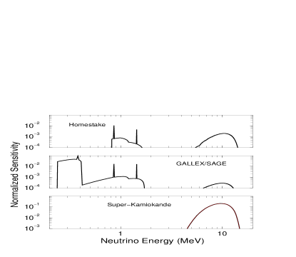
FIG. 1.: Spectral sensitivity as a function of the neutrino energy.

From Bayes’ theorem we compute the posterior probability $P({\cal P}|D,I)$, that is, the probability of the hypothesis $H$ that the set of parameters ${\cal P}\equiv({\cal P}_{1},\ldots,{\cal P}_{12})$ have specified values. For the Gallium rate we use the weighted average of the SAGE and GALLEX results. The posterior probability $P({\cal P}_{k}|D,I)$ for each ${\cal P}_{k}$ is obtained by marginalizing (that is, integrating) $P({\cal P}|D,I)$ over the remaining ${\cal P}_{k}$. We use the mean of $P({\cal P}_{k}|D,I)$ as our best estimate of ${\cal P}_{k}$. The results, assuming that the measured rate is produced by $\nu_{e}$ only, are shown in Fig. 2(a). We see that in the first two bins, that span the $pp$ neutrino spectrum, the survival probability is close to unity. There is a marked suppression in the bin (0.8-1.5 MeV) that contains the main ${}^{7}Be$ line and a moderate suppression in the ${}^{8}B$ spectrum (bins spanning 6-12 MeV). These results agree with previous analyses [7, 8]. But our result provides additional information, namely: the precision with which the survival probability is known—as a function of the neutrino energy, irrespective of the precise origin of the neutrino deficit. Moreover, since our binned method makes no assumption about the form of the survival probability it makes no unwarranted inferences. Where there is little spectral sensitivity (in the intervals 0.4-0.8 MeV and 1.5-4.5 MeV) our method infers correctly that little information can be extracted.

FIG. 2.: Our best estimate of the survival probability (dark dashed line) vs neutrino energy for the binned method assuming (a) the neutrino flux consists of $\nu_{e}$ only and (b)  $\nu_{e}$ plus $\nu_{\mu}$, due to oscillations. The 68.3% (shaded area) and 90% (solid line) confidence intervals, about our best estimate, are also shown.

If, however, we assume oscillations into active neutrinos ($\nu_{\mu}$) the inferred form of the survival probability changes. Figure 2(b) shows the extracted survival probability for such a case. Here, we see a marked suppression at a higher neutrino energy (i.e., at around 8.5 MeV).

In the parametric method, which is motivated by the conclusions of previous analyses [7, 8, 18], we write the survival probability as a sum of two finite Fourier series:

$${\cal P}(E_{\nu}|a) = \sum_{r=0}^{7}a_{r+1}\mbox{cos}(r\pi E_{\nu}/L_{1})$$ (6)

$$/ (1+\mbox{exp}[(E_{\nu}-L_{1})/b])$$ (7)

$$+ \sum_{r=0}^{3}a_{r+9}\mbox{cos}(r\pi E_{\nu}/L_{2}).$$ (8)

The first term in Eq. (4) is defined in the interval 0.0 to $L_{1}$ MeV—and suppressed beyond $L_{1}$ by the exponential, while the second term covers the interval 0.0 to $L_{2}$ MeV. We divide the function in this way so that it can accomodate a survival probability that varies rapidly in the interval 0.0 to $L_{1}$. Holding the parameters $L_{1}$, $L_{2}$ and $b$ fixed at 1.0, 15.0 and 0.1 MeV, respectively, we compute the posterior probability $P(a|D,I)$ for the parameters $a\equiv(a_{1},\ldots,a_{12})$. The data are the same as those used for the binned method; but instead of a linear sum in ${\cal P}_{k}$ we have a linear sum in the parameters $a$.

The theoretical uncertainties, which so far we have neglected, can be incorporated by treating the fluxes $\Phi\equiv(\Phi_{1},\ldots)$ as parameters with an associated prior probability, $P(\Phi|I)$, that encodes the flux predictions and whatever correlations exist amongst them. We represent our knowledge of the fluxes by a multivariate Gaussian prior probability $P(\Phi|I)=$ $g(\Phi|\Phi^{0},\Sigma_{\Phi})$, where $\Phi^{0}\equiv(\Phi_{1}^{0},\ldots,\Phi_{8}^{0})$ is the vector of flux predictions and $\Sigma_{\Phi}$ is the corresponding error matrix[19]. For simplicity we neglect correlations; hence $\Sigma_{\Phi}$ is diagonal.

The posterior probability (using a constant prior probability for the parameters $a$ is now given by $P(a,\Phi|D,I)=$ ${\cal L}(D|a,\Phi,I)$ $P(\Phi|I)$ $/\int_{a,\Phi}{\cal L}(D|a,\Phi,I)$ $P(\Phi|I)$, which when marginalized with respect to $\Phi$ gives $P(a|D,I)$. The survival probability is estimated using $P(E_{\nu}|D,I)=$ $\int_{a}{\cal P}(E_{\nu}|a)$ $P(a|D,I)$. Figure 3(a) shows the survival probability and its uncertainty, which now includes both the experimental and theoretical errors. Again, the general form of the survival probability obtained, assuming the neutrinos detected consist of $\nu_{e}$ only, agrees with the inferences from previous analyses and our binned method. But again, unlike previous analyses we have detailed information about the survival probability and its uncertainties as a function of the neutrino energy. Figure 3(b) shows our results, for the survival probability, assuming oscillations into active neutrinos.

One useful check of the reliability of both calculations, and the flexibility of the function in Eq. (4), is to set the measurements $D$ equal to their predicted values and to verify that the extracted survival probability is unity in the energy ranges where data exist and is 0.5 with an error of $\pm 0.3$ where there are no data. Both calculations have been verified successfully in this way.

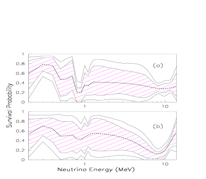
FIG. 3.: Survival probability vs neutrino energy for the parametric method assuming (a) the neutrino flux consists of $\nu_{e}$ only and (b) $\nu_{e}$ to $\nu_{\mu}$. All uncertainties are included. See Fig. 2 for other details.

We note the general agreement between the binned and parametric methods in the energy regions with adequate spectral sensitivity.

The calculations presented here are based on data from 1997. Our preliminary calculations using the data presented at the recent Neutrino ’98 conference[20], and the 1998 Bahcall and Pinsonneault predictions[21], yield similar conclusions, as illustrated in Fig. 4. The Bayesian method offers a well-founded way to compute the relative probabilities of different models of the survival probability. We plan to provide such calculations in a longer paper.

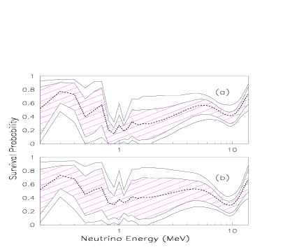
FIG. 4.: Survival probability vs neutrino energy for the parametric method using 1998 data and solar model[21]. All uncertainties are included. See Fig. 3 for other details.

In summary, we have used recent solar neutrino data and standard solar model predictions to extract the neutrino survival probability and its uncertainty as a function of the neutrino energy under two broad alternate assumptions: 1) the measured flux is comprised of $\nu_{e}$ only or 2) it is a mixture of active neutrinos arising from $\nu_{e}$ oscillations. Under assumption 1), we find that the survival probability is most precisely determined around 0.3 MeV and has a value of 0.79$\pm$0.13 (and 0.28$\pm$0.03 at 8.3 MeV) with experimental and theoretical uncertainties included. However, the uncertainties elsewhere are considerably larger. Our results suggest that the data could accomodate a wider range of models than hitherto have been considered. In particular, the fact that the MSW model provides a good description of the data is clearly a strong point in its favor; but it is at present not a decisive one. We therefore eagerly await further results from Super-Kamiokande and the first results from SNO[22].

The authors would like to thank John Bahcall for providing the latest theoretical information used in the present analysis and for useful suggestions and Robert Svoboda for providing the latest Super Kamiokande data. We acknowledge the support of the U.S. Department of Energy and U.S. National Science Foundation. Fermi National Accelerator Laboratory is operated by the Universities Research Association, under contract with the U.S. Department of Energy.

REFERENCES

- [1] J. N. Bahcall and M. Pinsonneault, Rev. Mod. Phys. 67, 781 (1995), and references therein. J. N. Bahcall (private communication 1998).
- [2] “Neutrino Astrophysics,” J. N. Bahcall, (Cambridge University Press, 1989); http://www.sns.ias.edu/jnb/.
- [3] S. Turck-Chize and I. Lopes, Astrophys. J. 408, 347 (1993).
- [4] V.N. Gribov and B.M. Pontecorvo, Phys. Lett. B 28, 493 (1969); J.N. Bahcall and S.C. Frautschi, Phys. Lett. B 29, 623 (1969); S.L. Glashow and L.M. Krauss, Phys. Lett. B 190, 199 (1987).
- [5] L. Wolfenstein, Phys. Rev. D 17, 2369 (1978); S.P. Mikheyev and A.Yu. Smirnov, Sov. J. Nucl. Phys. 42, 913 (1986); Nuovo Cimento C 9, 17 (1986).
- [6] J. N. Bahcall, Astrophys. J. 467, 475 (1996).
- [7] N. Hata and P.Langacker, Phys. Rev. D 50, 632 (1994), N. Hata and P.Langacker, Phys. Rev. D 56, 6107 (1997).
- [8] Q. Y. Liu and S. T. Petcov, Phys. Rev. D 56, 7392 (1997); A.B. Balantekin, J.F. Beacom, J.M. Fetter, Phys. Lett. B 427, 317 (1998).
- [9] E. Gates, L.M. Krauss, M. White, Phys. Rev. D 51, 2631 (1995).
- [10] J. N. Bahcall et al., Phys. Rev. C 54, 411 (1996).
- [11] J. N. Bahcall, “The Inconstant Sun,” 2nd Napoli Thinkshop on Physics and Astrophysics, Napoli, 18 March 1996, eds. G. Cauzzi and C. Marmolino, Memorie Della Societ Astronomica Italiana, 68 N. 2, 1997, pp. 361-368.
- [12] Homestake Collaboration, K. Lande, in the 4th International Solar Neutrino Conference, Heidelberg, Germany, 1997, to appear in the Proceedings; B. T. Cleveland et al., Nucl. Phys. B 38, 37 (1995).
- [13] GALLEX Collaboration, P. Anselmann et al., Phys. Lett. B 327, 377 (1995); W. Hampel et al., Phys. Lett. B 388, 384 (1996).
- [14] SAGE Collaboration, in LP ’97, International Symposium on Lepton Photon Interactions, Hamburg, Germany, 1997, to appear in Proceedings.
- [15] Y. Takeuchi, Super-Kamiokande results presented at Moriond, France, March 1997, to appear in the Proceedings; Nucl. Phys. B 38, 54 (1995).
- [16] We have used the data given in Table II of the paper by G. L. Fogli et al., Astro. Part. Phys. 9, 1119 (1998).
- [17] J. N. Bahcall et al., Phys. Rev. D 51, 6146 (1995).
- [18] C.M. Bhat, 8th Lomonosov Conference on Elementary Particle Physics, Moscow, Russia, August 1997, to appear in proceedings, FERMILAB-Conf-98/066; C.M. Bhat et al., Proceedings of the 9th Meeting of the DPF of the American Physical Society, ed. K. Heller et al. (World Scientific, 1996) p.1220; S. Parke, Phys. Rev. Lett. 74, 839 (1995).
- [19] J. N. Bahcall and P. I. Krastev, Phys. Rev. D 53, 4211 (1996). We take the larger of the positive and negative errors. We have not included 10% [2] uncertainties in the absorption cross sections for the experiments.
- [20] K. Lande (Homestake), V.N. Gavrin (SAGE), T. Kirsten (GALLEX) and Y. Suzuki (Super-Kamiokande), NEUTRINO ’98 Takayama, Japan (1998), http://www-sk.icrr.u -tokyo.ac.jp/nu98; Robert Svoboda, private communication 1998.
- [21] J. N. Bahcall et al., (To be published in Phys. Rev. D); J. N. Bahcall et al., Phys. Lett. B 433, 1 (1998).
- [22] A. B. McDonald, in Proceedings of the 9th Lake Louise Winter Institute, ed. A. Astbury et al. (World Scientific, 1994) p.1; http://snodaq.phy.queensu.ca/SNO /sno.html.