Semi-automated Extraction of Digital Objective Prism Spectra

Abstract

We describe a method for the extraction of spectra from high dispersion objective prism plates. Our method is a catalogue driven plate solution approach, making use of the Right Ascension and Declination coordinates for the target objects. In contrast to existing methods of photographic plate reduction, we digitize the entire plate and extract spectra off-line. This approach has the advantages that it can be applied to CCD objective prism images, and spectra can be re-extracted (or additional spectra extracted) without having to re-scan the plate. After a brief initial interactive period, the subsequent reduction procedure is completely automatic, resulting in fully-reduced, wavelength justified spectra. We also discuss a method of removing stellar continua using a combination of non-linear filtering algorithms.

The method described is used to extract over 12,000 spectra from a set of 92 objective prism plates. These spectra are used in an associated project to develop automated spectral classifiers based on neural networks.

1 Introduction

The MK classification of stellar spectra (Morgan, Keenan & Kellman 1943) has been an important tool in the workshop of stellar and galactic astronomers for more than a century. While improvements in astrophysical hardware have enabled the rapid observation of digital spectra, our ability to efficiently analyze and classify spectra has not kept pace. Traditional visual classification methods are clearly not feasible for large spectral surveys. In response to this, we have been working on a project to develop automated spectral classifiers (von Hippel et al. 1994; Bailer-Jones 1996; Bailer-Jones et al. 1997, 1998). These classifiers, which are based on supervised artificial neural networks, can rapidly classify large numbers of digital spectra.

The development of these classification techniques has required a large, representative set of previously classified spectra. The most suitable data has been the spectra from the Michigan Spectral Survey (Houk 1994) and the accompanying MK spectral type and luminosity class classifications listed in the Michigan Henry Draper (MHD) catalogue (Houk & Cowley 1975; Houk 1978, 1982; Houk & Smith-Moore 1988). This paper describes the data reduction techniques we developed to extract and process these spectra.

2 Plate Material

The Michigan Spectral Survey was an objective prism survey of the whole southern sky ($\delta<12^{\circ}$) from the Curtis Schmidt Telescope at the Cerro Tololo Interamerican Observatory in Chile. We scanned a number of the plates from this survey using the APM facility in Cambridge (Kibblewhite et al. 1984). This machine uses a flying-spot laser and photomultiplier detector to digitize areas of the plate. The usual mode of use for prism plates is to locate objects using their known co-ordinates and then to scan just the region of interest, either by recording all of the pixels or by parametrizing the object in real time (e.g. Hewett et al. 1985). The coordinates are often obtained from a direct image of the same field taken on the same telescope. Other groups have also developed methods for the automated and semi-automated extraction of prism spectra (e.g. Clowes, Cooke & Beard 1984; Flynn & Morrison 1990; Hagen et al. 1995; Wisotzki et al. 1996) often with the goal of identifying quasar spectra.

Our approach differs from the conventional method in the principal respect that we used the APM in raster scanning mode to digitize the entire plate. Subsequent plate reduction and extraction of the spectra take place off-line. The main reason for this approach is that it can equally well be applied to CCD objective prism images, which are increasingly replacing photographic plates. Furthermore, additional spectra can later be extracted very rapidly without requiring access to a plate scanning machine. Tests determined that the optimal scanning resolution was 15 $\mu m$, which corresponds to 1.45” per pixel. While the site seeing is typically better, the telescope has relatively poor tracking ability, and this led to an effectively lower seeing (blurring). Table 1 gives details of the plates and the reduced spectra. Figure 1 shows a typical plate.

Table 1: Details of the plates and the extracted spectra.

Plate type	IIaO
Plate size	$\approx 20\times 20cm$
	$\approx 5^{\circ}\times 5^{\circ}$
	12,000 $\times$ 12,000 pixels
	289 Mb (FITS)
Plate scale	96.62 arcsec $mm^{-1}$
Dispersion	108 Å/mm at H$\gamma$
Scanning pixel size	15$\mu$m
	$\Rightarrow$ 1.45 arcsec $pix^{-1}$
	$\Rightarrow$ 1.6 Å $pix^{-1}$ at H$\gamma$
	(1.05 Å $pix^{-1}$ @ 3802 Å
	2.84 Å $pix^{-1}$ @ 5186 Å)
Time to digitize one plate	100 minutes
Coverage of final spectra	3802–5186 Å
Magnitude limit of plates	B $\sim 12$
Number of stars on 92 plates	$\approx 16,000$

Figure 1: (This figure is supplied as a separate JPEG file.) APM negative image of a 5^∘ objective prism plate from the Michigan Spectral Survey.

As with the conventional APM method, we extract known objects on the basis of their coordinates. However, due to the absence of any appropriate direct plate material from which $x,y$ coordinates could be obtained, we used catalogue $\alpha,\delta$ coordinates of our target objects. We discovered that the MHD $\alpha,\delta$ positions were unreliable compared with those in the Positions and Proper Motions (PPM) catalogue (Röser & Bastian 1991), with an average discrepancy of $\approx 20^{\prime\prime}$. (The positions in the PPM South catalogue have mean random errors of $0.1^{\prime\prime}$.) Hence where cross identifications between the MHD and PPM catalogue entries were available (for about 85% of the stars in the MHD) we used the PPM coordinates. Co-ordinates could of course be used from any other source catalogue. Furthermore, because the MHD is incomplete ($\sim 50\%$ of all stars down to $B\sim 11$) we supplemented it with all PPM stars not listed in the MHD. This supplement not only permits extraction of more spectra, but helps us identify overlaps between neighbouring spectra.

3 Image Reduction and Spectral Extraction

An objective prism disperses the light from every point in the field of view, with the result that the spectra on the detector lack a common wavelength zero point (Figure 1). Thus the reduction procedure must pay careful attention to the mutual wavelength alignment (justification) of the spectra. Another complication is that because the plates were originally obtained for the purposes of visual classification, they have been widened, thus increasing the chance of overlaps between adjacent spectra. Finally, the $\alpha,\delta$ co-ordinates of the plate centres are only poorly known.

Given that we want to extract the spectra of objects with known $\alpha,\delta$ co-ordinates, our reduction approach is to use a subset of spectra to solve a parametrized mapping of the form $\alpha,\delta$ $\Rightarrow$ $x,y$, and then to use this to obtain $x,y$ positions for all required objects on the plate. In this section we outline our plate solution approach which is sufficient to extract accurately aligned spectra. A full description is given in Bailer-Jones (1996).

3.1 Evaluate Plate Centre

A list of extraction targets for a given plate was drawn-up using the plate codes which appear for each star in the MHD catalogue. This list was supplemented with PPM stars not listed in the MHD catalogue on the basis of their $\alpha,\delta$ co-ordinates. The coordinates of the plate center, $\alpha_{\rm{c}},\delta_{\rm{c}}$, are only known to an accuracy of $\approx 1^{\circ}$, corresponding to $>20$% of the plate. Using this nominal centre, the tangent plane projections, $\xi,\eta$ (the standard coordinates), of the $\alpha,\delta$ positions of each star are obtained. Once suitably scaled, the $\xi,\eta$ co-ordinates are the plate $x_{1},y_{1}$ co-ordinates. From the full list of extraction targets, a subset, the $\Gamma_{1}$ spectra, is selected which will be used to define the first plate solution. These spectra are those which are bright and relatively isolated from other spectra, necessary to ensure their unambiguous identification. We cannot use all spectra for forming the plate solution at this stage on account of the poor nominal plate centre.

The only interactive part of this reduction method is an iterative procedure to improve the plate centre. By displaying the $x,y$ positions of the $\Gamma_{1}$ spectra over an image of the plate, the $\Delta x$, $\Delta y$ shifts required to improve the match between the spectra and positions are measured. Using these offsets to move the plate centre, the $\xi,\eta$ projections are recalculated and the procedure repeated (Figure 2). A good match can usually be obtained in two iterations, taking only a couple of minutes. A highly accurate plate centre is not required as the plate solutions include constant terms which accommodate small linear offsets in $x$ and $y$.

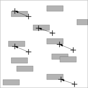
Figure 2: An $x,y$ offset is applied to the projected plate centre in order to achieve a better superimposition of the object positions with their spectra. This offset is determined visually. The grey boxes are a schematic representation of the spectra, and the crosses represent their initial and improved positions.

3.2 Marginal Sums and Cross-Correlation

With perfect telescope optics and an exact plate centre, the $\xi,\eta$ co-ordinates would be sufficient to extract all spectra with known $\alpha,\delta$ co-ordinates. However, due to optical distortions, a plate solution approach is needed. To achieve this, exact $x,y$ plate co-ordinates are required for the $\Gamma_{1}$ spectra.

Positions on the spectra are achieved using marginal sums, which locates the brightest point within a rectangular box. A box of size $800\times 300$ pixels is centered on the $x_{1},y_{1}$ position. The brightest point in this box is

$$x_{2}=\max_{i}S(i)=\max_{i}\left(\sum_{j=1}^{j=300}I_{i,j}\right)$$ (1)

and

$$y_{2}=\max_{j}S(j)=\max_{j}\left(\sum_{i=1}^{i=800}I_{i,j}\right)\ \ ,$$ (2)

where $I_{i,j}$ is the number of (sky-subtracted) flux counts in pixel $(i,j)$ (Figure 3). As the nominal position, $x_{1},y_{1}$, of the spectrum is uncertain, this box is considerably wider (300 pixels) than the width of the spectrum (about 50 pixels). The $y$-centre of the spectrum ($y_{3}$) is then located by fitting a top-hat to $S(j)$.

Figure 3: Marginal sums in a region around the nominal $x_{1},y_{1}$ position of the spectrum yields the position $x_{2},y_{2}$. The $y$-centre of the spectrum is found by fitting a top-hat across the spectral profile function, $S(j)$, and taking the centre of the top-hat to be the $y$-centre of the spectrum, $y_{3}$.

The marginal sum $S(i)$ is a noisy version of the spectrum. Thus the peak of $S(i)$, viz. $x_{2}$, differs for different spectral types (by $\approx 50$ pixels), whereas we need to identify the position of a common wavelength for all spectra. This is done by using the $x_{2},y_{3}$ positions to extract the $\Gamma_{1}$ spectra and then cross-correlating them with templates (the extraction process is described below). The position of this cross-correlation peak ($x_{3}$) corresponds to a common wavelength for all the $\Gamma_{1}$ spectra.

3.3 First Plate Solution

The $x_{3},y_{3}$ positions are used to solve the two-dimensional linear plate solution equations

$$x_{3}=a_{0}+a_{1}\eta+a_{2}\xi$$ (3)

and

$$y_{3}=b_{0}+b_{1}\eta+b_{2}\xi$$ (4)

for the 6 coefficients using Gauss–Jordan elimination (see, for example, Press et al. 1992).

Defining $x_{3}^{\prime}$ as the values used to solve equation 3 and $x_{3}$ as those obtained by applying the solution, the solution residual is defined by $x_{3}-x_{3}^{\prime}$, and similarly for $y_{3}$. The equations were solved iteratively by rejecting, at each iteration (up to a finite number of iterations), points which had residuals greater than $3\tilde{\sigma}$, where $\tilde{\sigma}$ is the average of the absolute value of the residuals. (If the residuals are distributed as a Gaussian this would be equivalent to $2.4\sigma$ clipping. The modulus error is less sensitive to outliers than the RMS error and so gives a more stable error estimate upon iteration.) The final solution always had more than 25 objects, which gave typical residuals of $\sigma_{x}\approx 10$ pixels and $\sigma_{y}\approx 1$ pixel. (These are not the final errors: spectral alignment is improved below.) Higher order solutions at this stage were found to be much less robust, on account of the increased number of parameters. Figure 4 shows a typical example of the residuals plotted as a function of plate position.

Figure 4: Typical residuals after applying the first (2-D linear) plate solution given by equations 3 and 4. The length of each arrow is proportional to the magnitude of the solution residual and the direction of the arrow gives the relative sizes of the $x$ and $y$ errors. The arrow at about (9500,4000) corresponds to a 2 pixel error.

3.4 Spectral Extraction

Once solved, equations 3 and 4 give $x,y$ positions for all spectra with known $\alpha,\delta$ co-ordinates. An extraction box of size $1020\times 200$ pixels is placed at each position and the apextract routine from iraf used to extract the spectra. Note that this extraction box is oversized in $y$ to ensure that the ends of a rotated spectrum were included within the box, as shown in Figure 5. This rotation ($\sim 1^{\circ}$) occurs because the prism was not perfectly aligned relative to the East-West axis of the telescope. Extraction is performed using apertures, based on the optimal extraction algorithm first introduced by Hewett et al. (1985) and subsequently generalized by Horne (1986). The aperture is a model for the cross-dispersion profile of the spectrum, with the optimum aperture at each point determined by a maximum likelihood procedure (e.g. Irwin 1997). Because the location of the spectrum has been well-determined in advance, it is guaranteed that the correct spectrum (as opposed to an adjacent brighter spectrum) is traced and extracted.

Figure 5: Spectral extraction. The target spectrum is centred within the extraction box. The spectrum is located, traced and extracted using constraints on the position of the spectrum already determined. Note that although the spectra are generally rotated relative to the $x$-edge of the plate, the dispersion axis is still parallel to the $x$-axis. The solid line in the plot to the right is a schematic of the profile at a point along the spectrum, and the dashed line the corresponding aperture.

Aperture fitting is done on sky subtracted pixels to increase the dynamic range available for fitting. On account of the prism, the sky background is grey and varies smoothly and slowly across the plate, and was found to be uniform over the scale of a single spectrum ($\approx 0.4^{\circ}$). The sky level is determined using an iteratively $k$-$\sigma$ clipped median of all pixels in the extraction box. Stellar pixels are preferentially removed with asymmetrical clipping ($k=1\sigma$ upper; $k=5\sigma$ lower). The approach would be invalid for very crowded regions where the pixels in the extraction box are mostly stellar ones. However, in such cases there are also large overlaps between the spectra making it very difficult to extract the spectra anyway.

3.5 Second Plate Solution

We now have a set of one-dimensional extracted spectra aligned to a precision of $\sigma_{x}\approx 10$ pixels. This is improved upon by locating a unique spectral feature (the H$\beta$ line) and using its position to solve a second plate solution. The H$\beta$ line is suitable on account of being both strong and well-isolated from other spectral lines in spectra earlier than about G5, thus easing unambiguous identification. A region is selected around the expected position of the line, the continuum removed and the spectrum inverted. The H$\beta$ line is assumed to be the strongest feature in this region which is at least $3\sigma$ above the background. The mean of a Gaussian fitted to the line is taken to be the position, $\Delta x$, of the H$\beta$ line relative to $x_{3}$. The spectra for which a line could be located (the $\Gamma_{2}$ spectra) were used to solve the second plate solution

$$\Delta x=c_{0}+c_{1}\eta+c_{2}\xi+c_{3}\eta\xi+c_{4}\eta^{2}+c_{5}\xi^{2}\ \ ,$$ (5)

This was again solved iteratively using Gauss–Jordan elimination, with approximately 50 spectra in the final solution. Typical mean residuals for a given plate were $\sigma_{\Delta x}\approx 1$ pixel, but a typical median residuals were $<0.5$ pixels (Figure 6). Higher order solutions were found to be less robust. Note that equation 5 assumes that the prism dispersion is constant across the plate. This could be relaxed using additional terms.

Figure 6: Typical residuals after applying the second (1-D quadratic) plate solution given by equation 5. The length of each arrow is proportional to the magnitude of the solution residual and the direction of the arrow gives the sign. The scale (length of arrows) is the same as in Figure 4.

On account of the magnitude of these errors, alignment shifts can be rounded-off to the nearest whole pixel. Alignment precisions of better than $0.5$ pixels require interpolation. One drawback of interpolation is that the noise in the resultant spectrum is correlated between the pixels. This can be problematic for subsequent analysis/classification algorithms. Moreover, alignment precision for our spectra is limited by our ignorance of the radial velocities of these stars. A typical line-of-sight velocity of 40 km s^-1gives a Doppler shift of $0.5$ Å at 4000 Å  which corresponds to $\approx 0.5$ pixels. Thus radial velocity variations across the spectra limits alignment to no better than $0.5$ pixels.

In principle, cross-correlation with spectral standards could have been used to align the spectra. However, the disadvantage of this approach is that it requires that we know the approximate spectral type in advance, so that the right standard can be selected. Furthermore, a plate solution allows us to accurately extract faint (low S/N) spectra which would give unreliable cross-correlations.

4 Post-Extraction Processing

The extracted spectra were cut to a final wavelength range of 3802–5186 Å, covered by 820 pixels. This was dictated by the QE of the telescope–prism–plate combination, and the need to retain at least the region between the Ca II H&K lines (at 3933.7 Å and 3968.5 Å) and H$\beta$ line (at 4861.3 Å) for use in the automated classifiers. The range was extended as far as there were still spectral features at a reasonable S/N. The IIaO emulsion ‘cut-off’ (where the response drops to 50% of the peak) occurs at 4900 Å, although as can be seen from Figure 8, the drop-off in response is slow. At the blue end, a blocking filter dramatically reduces the QE below 3850 Å.

Most spectra were well-extracted and aligned. In a few cases—particularly for crowded plates, i.e. at low Galactic latitudes—we discovered that some spectra overlapped with neighbouring spectra. These should ideally have been deselected at the beginning of the reduction process based on their proximity to other spectra, but they remained, presumably because the MHD catalogue (even supplemented with the PPM) is not complete. (Most of the plates were deliberately chosen to lie at high Galactic latitudes to minimize crowding.) A small fraction of spectra were also deselected if they had unusually low S/N ratios, possibly on account of a poor aperture fit during the spectral extraction. A number of spectra were also lost due to overlap with the edge of the plate. The total number of stars retained was 12,104 out of a possible 15,820 spectra present on the 92 plates and listed in the catalogues.

5 Continuum Removal

Continuum-free spectra are required for many modes of spectral analysis. For example, in stellar classification, although a genuine stellar continuum is closely related to the effective temperature of a star, the continuum received at a telescope’s detector is often distorted by interstellar reddening, atmospheric extinction and instrumental effects. A particular problem is the non-linear (and uncalibrated) response of the photographic emulsion.

There are many different ways in which a stellar continuum can be removed, but not all are suitable or reliable. One approach is to fit a polynomial or non-linear spline to the spectrum and then subtract it from the spectrum. However, the high order polynomial usually needed requires many data points for its definition and is therefore likely to be distorted by spectral lines. One improvement is to fit the continuum only in pre-defined ‘continuum windows’ (regions which are relatively line-free) (Zekl 1982), although the drawback here is that the approximate classification must be known in advance, as the location of these windows depends on spectral type. Another improvement is to fit the polynomial only to ‘high points’ in the spectrum, but this requires the distinction between continuum and line features which can be very difficult for later-type stars.

Continuum removal is a process which removes all of the slowly varying—low-frequency—information from a spectrum. An attractive approach is to take the Fourier transform of the spectrum, filter out the low-frequency components (high-pass filter) and then reverse-transform the spectrum back into wavelength space; this will remove all slowly varying features. The drawback of this Fourier technique is that the broad spectral lines contribute to the low-frequency components, so removing low frequencies alters some of the line profiles and equivalent widths. LaSala & Kurtz (1985) improve upon this basic Fourier method by defining a continuum by passing the Fourier-transformed spectrum through a low-pass filter and Fourier-transforming back the result. This gives a suitably smoothed version of the original spectrum. The original spectrum is then rectified by dividing it by this continuum. This appears to give very reliable results for spectral types earlier than M1, but the authors report that it “fail[s] catastrophically” for later types and extreme emission line stars, because in such cases the defined continuum can be negative in places.

We chose to use a combination of median and boxcar filtering of a spectrum to obtain its continuum. This is a non-linear method which overcomes the shortcomings of linear methods based on Fourier transforms. The first process is to filter the spectrum with a one-dimensional median filter. Median filtering is performed by replacing the flux in each pixel with the median value in a box of $M$ pixels centered on the pixel of interest. The resulting ‘spectrum’ will not be very smooth, as it is composed of a sequence of flux values from the original spectrum which were generally non-adjacent. This ‘spectrum’ is a non-linear transformation of the original spectrum. To smooth it, it is then boxcar filtered: This is like median filtering except that each pixel is replaced with the mean value in a box of size $N$. To obtain a reliable continuum at the ends of the spectrum, a pseudo-spectrum is created beyond each end by reflecting the spectrum about the end pixel. This gives better results than simply truncating the filter size near the ends. These combined filters produce a smooth continuum which is subtracted from the original spectrum to give a line-only spectrum. The sizes of the filter boxes depend on the scale over which the spectrum shows variations. For our 820-pixel sized spectra, the values $M$=101 and $N$=50 were found to be most suitable.

The continuum fits from this method are generally good, but are poor in the regions of broad lines. To overcome this problem, we masked (cut out) the strong lines prior to median filtering, as shown in Figure 7. The masked and unmasked continua produced on a range of spectral types are shown in Figure 8. It can be seen that the masked continua are better near the strong lines, particularly the hydrogen lines. The large filter sizes of the unmasked filtering reflected the width of the broad lines. With masking, these sizes were reduced to $M$=51 and $N$=25. The wavelength coverages of the masked regions are shown in Table 2.

Figure 7: Continuum evaluation by masking strong lines (schematic). The region of a strong line is cut from the spectrum, the remaining spectrum joined up, and a median filter passed across the spectrum. The resulting spectrum is then split at the point where the spectral line was, and the spectrum linearly interpolated across the gap. A linear boxcar filter is run across this, resulting in the stellar continuum.

Figure 8: Continuum fit and subtraction using median and boxcar filtering. For each spectral type the upper spectrum is the unrectified spectrum, the solid line superimposed on it is the continuum obtained using the masked filters, and the lower spectrum is the resultant continuum-subtracted spectrum. The dashed line above each spectrum shows the continuum obtained using unmasked filters. Note that the ‘unmasked’ continuum gives a poorer fit in the region of broad lines.

Table 2: Masked line regions in an improved median filtering.

H + others	3811–3853 Å
H + Fe I	3864–3908 Å
Ca II H&K	3924–3987 Å
H$\delta$	4078–4129 Å
CN G-band	4293–4320 Å
H$\gamma$	4325–4365 Å
H$\beta$	4837–4897 Å

Continuum fits at the redder ends of late-type stars are always poor: the presence of many molecular bands makes the definition of a ‘continuum’ rather meaningless, so we can only remove low frequency variations. The main concern of continuum removal should be to extract a continuum to ‘first order’ in a consistent way, so as to remove that continuum information which is not intrinsic to the stellar spectrum, such as that produced by instrumental effects. Provided this condition is met, the exact shape of the continuum which is subtracted is not that important. This is demonstrated by the quality of the classifications we achieve with the reduced spectra (Bailer-Jones et al. 1997).

A combination of masked median filtering and linear filtering generally gives better continuum fits than Fourier methods. Any Fourier continuum estimation method which involves filtering out the high frequency components of the power spectrum is equivalent to ‘blurring’ the original spectrum by convolving it (in the wavelength space) with a broad bell-shaped function. As such, the continuum will always be distorted by the presence of broad lines or rapid changes in the original continuum. This convolution is a linear operation, which is why Fourier methods are limited in the type of continua they give. Median filtering, on the other hand, is a non-linear operation and can therefore produce a better fit to the continuum. When followed up with a linear filter (boxcar), a smooth continuum is obtained. The combined median/boxcar filter is also robust and consistent, in the sense that it is not sensitive to data ‘spikes’ (unlike linear methods) and thus will give similar continua for similar spectral types even in the presence of bogus spectral features.

6 Summary

Figure 9: Distribution of spectral types for each luminosity class. The dotted line represent giants (III), the dashed line subgiants (IV) and the solid line dwarfs (V).

This paper has described a method for extracting spectra from objective prism images. The method has been developed for the reduction of a set of photographic objective prism plates, but because the spectral extraction and processing takes place entirely in software using the complete digitized plate, it can equally well be applied to CCD objective prism images. The extraction process is driven by a set of catalogue Right Ascension and Declination positions, so a direct image of each field is not required. After an initial interactive period taking one or two minutes, the subsequent reduction is automatic, taking approximately one hour on a modest-sized SUN Sparc IPX to process a single plate (i.e. extract about 150 spectra).

The reduction method described in this paper has been used to extract a set of over 12,000 high-quality spectra. From this, a subset of over 5,000 normal spectra was selected which had reliable two-dimensional (spectral type and luminosity class) classifications listed in the MHD catalogue. The frequency distribution of the various stellar classes in this set is shown in Figure 9. This data set is used in accompanying papers to produce automated systems for classifying and physically parametrizing stellar spectra (Bailer-Jones et al. 1997, 1998).

In the interests of extending spectral classification to more distant stellar populations, spectra of stars fainter than B $\sim 12$ are required. This could be achieved with a CCD objective prism survey. Although the technique described can only extract objects with known Right Ascension and Declination coordinates, the HST Guide Star Catalogue (e.g. Lasker et al. 1990), which lists 19 million objects brighter than 16^th magnitude, could be used as a driver for extraction. However, Bailer-Jones (unpublished, 1996) has also modified the method to extract unwidened spectra from CCD objective prism images in the absence of any coordinates, using an algorithm to locate local flux peaks. The method can be applied to spectra at different spectral resolutions and wavelength coverages, provided a suitable line exists for the second plate solution.

References

- [1] Bailer-Jones C.A.L., 1996, PhD thesis, Univ. Cambridge
- [2] Bailer-Jones C.A.L., Irwin M., Gilmore G., von Hippel T., 1997, MNRAS, 292, 157
- [3] Bailer-Jones C.A.L., Irwin M., von Hippel T., von Hippel T., 1998, MNRAS, in press
- [4] Clowes R.G., Cooke J.A., Beard S.M., 1984, MNRAS, 207, 99
- [5] Flynn C., Morrison H.L., 1990, AJ, 100, 1181
- [6] Hewett P.C., Irwin M.J., Bunclark P., Bridgeland M.T., Kibblewhite E.J., He X.T., Smith M.G., 1985, MNRAS, 213, 971
- [7] Horne K., 1986, PASP, 98, 609
- [8] Houk N., 1978, University of Michigan Catalogue of Two-Dimensional Spectral Types for the HD Stars. Vol. 2: Declinations -53 to -40 degrees
- [9] Houk N., 1982, University of Michigan Catalogue of Two-Dimensional Spectral Types for the HD Stars. Vol. 3: Declinations -40 to -26 degrees
- [10] Houk N., Cowley A.P., 1975, University of Michigan Catalogue of Two-Dimensional Spectral Types for the HD Stars. Vol. 1: Declinations -90 to -53 degrees
- [11] Houk N., Smith-Moore M., 1988, University of Michigan Catalogue of Two-Dimensional Spectral Types for the HD Stars. Vol. 4: Declinations -26 to -12 degrees
- [12] Houk N., 1994, in Corbally C.J., Gray R.O., Garrison R.F., eds, Astronomical Society of the Pacific Conference Series 60, The MK Process at 50 Years. Astronomical Society of the Pacific, San Francisco, p. 285
- [13] Hagen H.-J., Groote D., Engels D., Reimers D., 1995, A&AS, 111, 195
- [14] Irwin M.J., 1997, in Espinosa J.M. ed., Canary Islands Winter School, Instrumentation for Large Telescopes, in press
- [15] Kibblewhite E.J., Bridgeland M.T., Bunclark P.S., Irwin M.J., 1984, in Kinglesmith D.A., ed, NASA-2317, Astronomical Microdensitometry Conference. NASA, Washington D.C., p. 227
- [16] LaSala J., Kurtz M.J., 1985, PASP, 97, 605
- [17] Lasker B.M., Sturch C.R., McLean B.J., Russell J.L., Jenkner H., Shara M.M., 1990, AJ, 99, 2019
- [18] Morgan W.W, Keenan P.C., Kellman E., 1943, An Atlas of Stellar Spectra with an Outline of Spectral Classification. University of Chicago Press, Chicago
- [19] Press W.H., Teukolsky S.A., Vetterling W.T., Flannery B.P., 1992, Numerical Recipes, 2nd edn. Cambridge Univ. Press, Cambridge
- [20] Röser S., Bastian U., 1991, PPM Star Catalogue, vols. 1 and 2. Spektrum Akademischer Verlag, Heidelberg
- [21] von Hippel T., Storrie-Lombardi L., Storrie-Lombardi M.C., Irwin M., 1994, MNRAS, 269, 97
- [22] Wisotzki L., Koehler T., Groote D., Reimers D., 1996, A&AS, 115, 227
- [23] Zekl H., 1982, A&A, 108, 380