A COUNTS-IN-CELLS ANALYSIS OF LYMAN-BREAK GALAXIES AT REDSHIFT $Z\sim 3$

Abstract

We have measured the counts-in-cells fluctuations of 268 Lyman-break galaxies with spectroscopic redshifts in six 9${}^{\prime}~{}$$\times$ 9${}^{\prime}~{}$fields at $z\sim 3$. The variance of galaxy counts in cubes of comoving side length 7.7, 11.9, 11.4 $h_{100}^{-1}$ Mpc is $\sigma_{\rm gal}^{2}\sim 1.3\pm 0.4$ for $\Omega_{M}=1$, $0.2$ open, $0.3$ flat, implying a bias on these scales of $\sigma_{\rm gal}/\sigma_{\rm mass}=6.0\pm 1.1$, $1.9\pm 0.4$, $4.0\pm 0.7$. The bias and abundance of Lyman-break galaxies are surprisingly consistent with a simple model of structure formation which assumes only that galaxies form within dark matter halos, that Lyman-break galaxies’ rest-UV luminosities are tightly correlated with their dark masses, and that matter fluctuations are Gaussian and have a linear power-spectrum shape at $z\sim 3$ similar to that determined locally ($\Gamma\sim 0.2$). This conclusion is largely independent of cosmology or spectral normalization $\sigma_{8}$. A measurement of the masses of Lyman-break galaxies would in principle distinguish between different cosmological scenarios.

1 INTRODUCTION

Much of observational cosmology depends upon the assumption that the spatial distribution of galaxies is related in a simple way to the underlying distribution of matter. At first it was hoped that the galaxy distribution might simply be a Poisson realization of the matter distribution; but as this model became difficult to reconcile with large scale peculiar velocities, the amplitude of microwave background fluctuations, the different clustering strengths of different galaxy types, and theoretical prejudice for $\Omega_{M}=1$, cosmologists began to assume an unspecified constant of proportionality $b$ between galaxy and mass fluctuations: $\delta_{\rm gal}=b\delta_{\rm mass}$. Though many physical processes could in principle give rise to a relationship of this form (e.g. Dekel & Rees 1987), most were poorly understood, and, if invoked, would make it difficult to use galaxy observations to constrain the cosmological mass distribution. An important exception was gravitational instability. This is relatively well understood, and if it were dominant in determining where galaxies formed—if galaxies formed within virialized “halos” of dark matter, and if the poorly understood physics of star formation, supernova feedback, and so on were important only in determining the properties of galaxies within dark matter halos—then the large scale distribution of galaxies would still be related in a simple way to the underlying distribution of matter; the value of the “bias parameter” $b$ in $\delta_{\rm gal}=b\delta_{\rm mass}$ would be straightforward to calculate (White & Rees 1978, Kaiser 1984, Bardeen et al. 1986, Mo & White 1996). Because it maintains a simple relationship between galaxies and mass, agrees with our limited knowledge of the relevant physics, and seems consistent with numerical simulations, this “dark halo” model has become increasingly popular, and is now the basis of the modern understanding of galaxy formation. It is assumed in most analytic treatments, in semi-analytic models, and in numerical simulations which include only gravity; and yet it remains a conjecture that has never been thoroughly tested. One prediction of the dark halo model is that galaxies of a given mass should form first in regions where the density is highest, and since such regions are expected to be strongly clustered (e.g. Kaiser 1984), a natural test is to measure the clustering of galaxies in the young universe.

The Lyman-break technique (e.g., Steidel, Pettini, & Hamilton 1995) provides a way to find large numbers of star-forming galaxies at $z\sim 3$. Star-forming galaxies have pronounced breaks in their spectra at 912 Å (rest) from a combination of absorption by neutral hydrogen in their interstellar media and the intrinsic spectra of massive stars. At $z\lower 2.15277pt\hbox{$\;\buildrel>\over{\sim}\;$}3$ this “Lyman break,” strengthened from additional absorption by hydrogen in the unevolved intergalactic medium, is redshifted sufficiently to be observed with ground-based broad-band photometry. By taking images through filters that straddle the redshifted Lyman break, and looking for objects that are much fainter in images at wavelengths shortward of the break than longward of the break, one can efficiently separate high-redshift galaxies from the many foreground objects. In our implementation of the technique, we have used deep photometry in the custom $U_{n}$, $G$, ${\cal R}$ filter system of Steidel & Hamilton (1993) to assemble a sample of over 1300 probable $z\sim 3$ galaxies, of which more than 400 have been spectroscopically confirmed with the Low-Resolution Imaging Spectrograph (Oke et al. 1995) on the W. M. Keck telescopes.

After initial spectroscopy in one 9${}^{\prime}~{}$$\times$ 18${}^{\prime}~{}$field, we argued, on the basis of a single large concentration of galaxies, that these $z\sim 3$ Lyman-break galaxies were much more strongly clustered than the mass, with an inferred bias parameter $b\equiv\sigma_{\rm gal}/\sigma_{\rm mass}$ of $b\lower 2.15277pt\hbox{$\;\buildrel>\over{\sim}\;$}6$, $2$, $4$ for $\Omega_{M}=1$, $0.2$ open, and $0.3$ flat (Steidel et al. 1998a). Qualitatively this strong biasing was consistent with the idea that galaxies form first in the (strongly clustered) densest regions of the universe, but there appeared to be quantitative problems. In the dark matter halo model there is an inverse relationship between the abundance and bias of a population of halos, with the rarest, most massive halos being the most strongly clustered (i.e., most “biased”). As emphasized by Jing & Suto (1998), for halos to be as strongly clustered as Lyman-break galaxies, they would have to be very rare indeed. Yet Lyman-break galaxies are not that rare; for $\Omega_{M}=1$ their comoving number density to ${\cal R}=25.5$ is $n\lower 2.15277pt\hbox{$\;\buildrel>\over{\sim}\;$}8\times 10^{-3}$ per $h_{100}^{-3}$ Mpc³, comparable to the number density of $L_{*}$ galaxies today. As we will see below, in standard ($\Omega_{M}=1$, $\sigma_{8}=0.6$, $\Gamma=0.50$) CDM, halos at $z\sim 3$ with the same abundance as observed Lyman-break galaxies have a bias of $b\sim 4$, substantially lower than the implied galaxy bias. For $\Omega_{M}<1$ the disagreement is less severe, because both the estimated bias and the comoving abundance of observed Lyman-break galaxies are lower. It appeared then from preliminary analyses that our data were consistent with the dark halo model only for $\Omega_{M}<1$; but it was unclear how seriously to take conclusions based on a single feature in a single field. Moreover other authors soon analyzed the overdensity differently and argued that it was consistent with models in which galaxies are significantly less clustered than we claimed, with $b$ low enough to remove the inconsistencies with the abundances for $\Omega_{M}=1$ (e.g. Bagla 1997, Governato et al. 1998, Wechsler et al. 1998).

In this paper we present a counts-in-cell analysis of the clustering of 268 Lyman-break galaxies (all with spectroscopic redshifts) in six 9${}^{\prime}~{}$$\times$ 9${}^{\prime}~{}$fields. This sample contains four times as many galaxies over an area three times as large as our original analysis. Since in addition it takes into account all galaxy fluctuations in the data, and not just a single over-density, one might hope it would provide a more definitive measurement of the strength of clustering.

2 DATA

Many relevant details of our survey for Lyman-break galaxies are presented elsewhere (Steidel et al. 1996, Giavalisco et al. 1998a, Steidel et al. 1998a, Steidel et al. 1998b), and in this section we give only a brief review. We initially identify $z\sim 3$ galaxy candidates in deep $U_{n}$, $G$, ${\cal R}$ images taken (primarily) at the Palomar 5m Hale telescope with the COSMIC prime focus camera. In images of our typical depths (1$\sigma$ surface brightness limits of 29.1, 29.2, 28.6 AB magnitudes per arcsec² in $U_{n}$,$G$, and ${\cal R}$) approximately 1.25 objects per arcmin² meet our current selection criteria of

$${\cal R}\leq 25.5,\quad G-{\cal R}\leq 1.2,\quad U_{n}-G\geq G-{\cal R}+1,\quad U_{n}-G\geq 1.6.$$

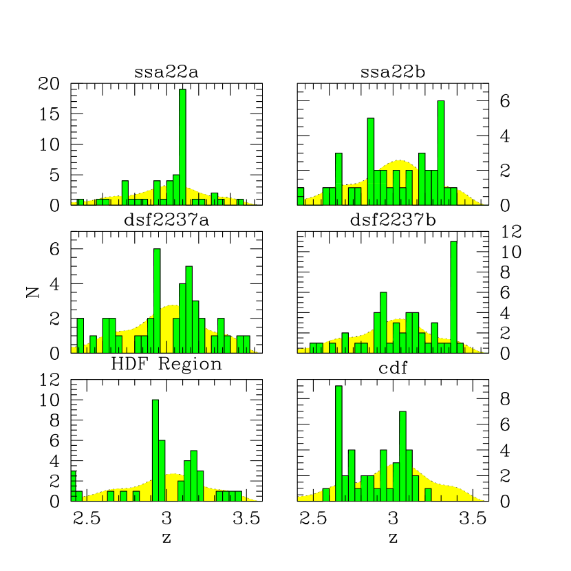
Figure 2: Redshift distributions in the six fields. The smooth curve is our estimated selection function, produced by fitting a spline to the coarsely binned redshifts of all candidates matching our selection criteria; the superimposed histograms are the measured redshifts in each field. The actual binning used in our analysis is somewhat different from the binning presented here. The average number of redshifts per field is about 44, with field to field variations due mainly to different levels of spectroscopic completeness.

A subset of these photometric candidates is subsequently observed spectroscopically at the W. M. Keck telescope through multislit masks which accommodate $\sim 20$ objects each. To date we have obtained spectra of 540 objects satisfying the above photometric criteria; 376 of these have been identified as galaxies (of which a very small fraction show evidence of AGN activity), with a redshift distribution shown in Figure 1; 18 are stars; and the remainder have not been identified because of inadequate signal to noise ratio. In this paper we restrict our analysis to the 268 Lyman-break galaxies in our six most densely sampled $\sim$ 9${}^{\prime}~{}$$\times~{}$9${}^{\prime}~{}$ fields, including more complete data in the “SSA22” field analyzed in Steidel et al. 1998a. The redshift histograms these six fields are shown in Figure 2; each field is treated independently in the analysis that follows, although in two cases (SSA22 and DSF2237) pairs of 9${}^{\prime}~{}$fields are adjacent on the plane of the sky.

3 STATISTICAL ANALYSIS

The strength of clustering can be estimated by placing galaxies into spatial bins (“cells”) and looking at the fluctuations in galaxy counts from cell to cell. A convenient measure of the clustering strength is

$$\sigma_{\rm gal}^{2}\equiv{1\over V_{\rm cell}^{2}}\int\int_{V_{\rm cell}}dV_{1}dV_{2}\xi_{g}(r_{12})$$

where $\xi_{g}(r)$ is the galaxies’ two-point correlation function. If there were large numbers of galaxies in each cell, so that shot noise were negligible, $\sigma_{\rm gal}^{2}$ would just be equal to the relative variance of galaxy counts in cells of volume $V_{\rm cell}$: $\sigma_{\rm gal}^{2}=<(N-\mu)^{2}>/\mu^{2}$, where $N$ is the observed and $\mu$ the mean number of galaxies in a cell. In practice shot noise makes a significant contribution to the variance of cell counts, and this contribution must be removed to estimate $\sigma_{\rm gal}^{2}$:

$$\sigma_{\rm gal}^{2}=(<(N-\mu)^{2}>-\mu)/\mu^{2}$$

(Peebles 1980, §36). For any cell the expected number of galaxies can be estimated accurately as $\mu\simeq N_{\rm tot}\phi(z)\Delta z$, where $\phi(z)$ is our selection function, determined by fitting a spline to the coarsely binned redshifts of all $\sim 400$ Lyman-break galaxies which satisfy our current color criteria and have redshifts, and $N_{\rm tot}$ is the number of galaxies in the field with redshifts. ($N_{\rm tot}$ varies from field to field because of differing spectroscopic completeness.) In general the uncertainty in cell count $N$ will dominate the uncertainty in $\mu$. If we neglect the relatively small uncertainty in $\mu$, we can estimate $\sigma_{\rm gal}^{2}$ from the number of counts $N$ in a single cell as

$${\cal S}=((N-\mu)^{2}-\mu)/\mu^{2}.$$

If $\mu$ were perfectly known, ${\cal S}$ would have expectation value $<{\cal S}>=\sigma_{\rm gal}^{2}$ and variance

$$<{\cal S}^{2}>-<{\cal S}>^{2}=2\sigma_{\rm gal}^{4}+4\sigma_{\rm gal}^{2}/\mu+(2+7\sigma_{\rm gal}^{2})/\mu^{2}+1/\mu^{3}$$

where we have used results in Peebles (1980, §36) and neglected the integrals over the three- and four-point correlation functions. In fact ${\cal S}$ will be a slightly biased estimator of $\sigma_{\rm gal}^{2}$, since our estimate of $\mu$ depends weakly on $N$ (through its contribution to $N_{\rm tot}$), but this bias should be small compared to the variance—which is itself only approximately equal to the RHS of equation 1. With ${\cal S}$ we can estimate $\sigma_{\rm gal}^{2}$ from the observed number of counts in a single cell; by combining the estimates ${\cal S}$ from every cell in our data with inverse-variance weighting, we arrive at our best estimate of $\sigma_{\rm gal}^{2}$. (The variance depends on the unknown $\sigma_{\rm gal}^{2}$, of course, but the answer converges with a small number of iterations.)

Placing our counts into a dense grid of roughly cubical cells whose transverse size is equal to the field of view ($\sim$ 9${}^{\prime}~{}$), we estimate $\sigma_{\rm gal}^{2}=1.3\pm 0.4$ in cells of approximate length 7.7, 11.9, 11.4 $h_{100}^{-1}$ Mpc for $\Omega_{M}=1$, $0.2\,{\rm open}$, $0.3\,{\rm flat}$. The uncertainty is the standard deviation of the mean of ${\cal S}$ estimated in the fields individually.

This approach with the estimator ${\cal S}$ has the advantage of being relatively model independent, but statisticians have long argued that an optimal data analysis must use the likelihood function (e.g. Birnbaum 1962). If we had a plausible model for the probability density function (PDF) of galaxy fluctuations $P(\delta_{\rm gal}|\sigma_{\rm gal}^{2})$, we might hope to produce a better estimate of $\sigma_{\rm gal}^{2}$ by finding the value that maximizes the likelihood of the data. An exact expression for the galaxy PDF has not been found, but it should be sufficient to use a reasonable approximation. The main requirement for this approximate PDF is that it be skewed, since a galaxy fluctuation $\delta_{\rm gal}\equiv(\rho_{\rm gal}-\bar{\rho}_{\rm gal})/\bar{\rho}_{\rm gal}$ can be arbitrarily large but cannot be less than -1. A particularly simple distribution with the necessary skew, the lognormal, provides a good fit to the PDF of mass fluctuations and of linearly biased galaxies in N-body simulations (e.g. Coles & Jones 1991, Coles & Frenk 1991, Kofman et al. 1994). The lognormal probability of observing a galaxy fluctuation $\delta_{\rm gal}$ given $\sigma_{\rm gal}^{2}$ is

$$P_{LN}(\delta_{\rm gal}|\sigma_{\rm gal}^{2})={1\over 2\pi x}\exp\biggl{[}-{1\over 2}\biggl{(}{\log(1+\delta_{\rm gal})\over x}+{x\over 2}\biggr{)}^{2}\biggl{]}$$

where $x\equiv\sqrt{\log(1+\sigma_{\rm gal}^{2})}$, and so in this model, assuming Poisson sampling, the likelihood of observing $N$ galaxies in a cell when $\mu$ are expected is

$$P(N|\mu\sigma_{\rm gal}^{2})=\int_{-1}^{\infty}d\delta_{\rm gal}P_{LN}(\delta_{\rm gal}|\sigma_{\rm gal}^{2})\exp[-(1+\delta_{\rm gal})N](1+\delta_{\rm gal})^{N}\mu^{N}/N!.$$

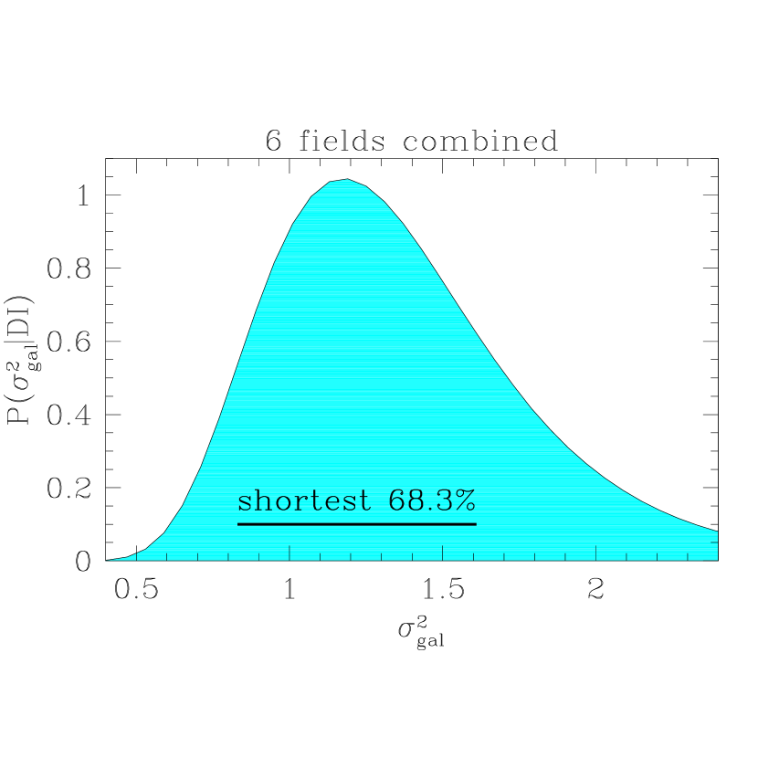
Figure 3: The posterior probability of our data as a function of clustering strength $\sigma_{\rm gal}^{2}$. A uniform prior in $\sigma_{\rm gal}^{2}$ is assumed, and the shortest 68% credible interval is shown.

The analytical solution to this integral is unknown, but it presents no numerical challenge. If the cells are large enough to be nearly uncorrelated, we can find the maximum likelihood value of $\sigma_{\rm gal}^{2}$ by maximizing the product of the likelihoods from individual cells. Figure 3 shows the product of the likelihoods for $\sigma_{\rm gal}^{2}$ from all cells in all six fields for $\Omega_{M}=1$. The plots for $\Omega_{M}=0.2\,{\rm open}$ and $\Omega_{M}=0.3\,{\rm flat}$ are similar, with small differences arising because our desire for cubical cells forces us to use different redshift binning for different cosmologies. For each cosmology the overall maximum likelihood value is close to $\sigma_{\rm gal}^{2}\sim 1.3$; the 68.3% credible intervals are 0.8 to 1.6, 0.7 to 1.4, and 1.1 to 2.1 for $\Omega_{M}=1$, $\Omega_{M}=0.2$ open, and $\Omega_{M}=0.3$ flat, in reasonable agreement with our estimate from ${\cal S}$. We will take the maximum likelihood estimates as our best estimates of $\sigma_{\rm gal}^{2}$ hereafter.

A more common measure of the clustering strength is the characteristic length $r_{0}$ in a correlation function of assumed form $\xi_{g}(r)=(r/r_{0})^{-\gamma}$. For spherical cells $r_{0}$ and $\sigma_{\rm gal}^{2}$ are related through $\sigma_{\rm gal}^{2}=72(r_{0}/R_{\rm cell})^{\gamma}/[(3-\gamma)(4-\gamma)(6-\gamma)2^{\gamma}]$ (Peebles 1980 §59), and so approximating our cubical cells as spheres with equal volume, and assuming $\gamma=1.8$, we arrive at a rough estimate of $r_{0}\simeq 4\pm 1$, $5\pm 1$, $6\pm 1$ comoving $h_{100}^{-1}$ Mpc for $\Omega_{M}=1$, $0.2$ open, $0.3$ flat. These values are large, comparable to the correlation lengths of massive galaxies today.

The correlation lengths for $\Omega_{M}=1$ and $\Omega_{M}=0.2$ open are larger, by about $2\sigma$, than those recently derived by Giavalisco et al. (1998a, “G98a” hereafter) from the angular clustering of Lyman-break galaxies. This discrepancy could be resolved in several ways. The correlation lengths would agree at the $1\sigma$ level if a large fraction of the objects whose spectra we cannot identify (about 25% of the spectroscopic sample) were lower redshift interlopers diluting the angular clustering signal. The discrepancy would also be reduced if $\gamma$ were larger than 1.8, although $\gamma$ would have to be equal to $\sim 2.6$, contradicting the results of G98a, to make the correlation lengths agree at the $1\sigma$ level. Because the spectroscopic subsample is somewhat brighter than the sample as a whole, one would expect (from arguments we develop below) the galaxies analyzed here to be somewhat more strongly clustered than those analyzed in G98a, but this would change $r_{0}$ by only $\sim$ 10-20% (these numbers follow from the formalism presented below, and will be explained more fully in Giavalisco et al. (1998b)). Inferring $r_{0}$ from observed angular clustering depends upon the assumed cosmological geometry, because (for example) projection effects must be corrected, and an intriguing possibility is that the correlation lengths disagree because G98a assumed an incorrect geometry when deriving $r_{0}$ from the angular clustering. According to G98a, the quantity $A^{1/\gamma}$ (for a correlation function of the assumed form $\omega(\theta)=A\theta^{1-\gamma}$) is well constrained by their observations. If we take $A^{1/\gamma}$ and $\sigma_{\rm gal}^{2}$ as two cosmology-independent parameters fixed by observation (which is not quite true; see above), then the correlation length derived from $\omega(\theta)$ scales with cosmological parameters roughly as $r_{0,\omega}\propto(g(\bar{z})/f^{1-\gamma}(\bar{z}))^{1/\gamma}$, where $g\equiv dl/dz$ is the change in proper distance with redshift and $f$ is the angular diameter distance, while the correlation length derived from $\sigma_{\rm gal}^{2}$ roughly obeys $r_{0,\sigma^{2}}\propto f(\bar{z})$. The ratio of these correlation lengths therefore depends on the geometry as $r_{0,\omega}/r_{0,\sigma^{2}}\propto(g/f)^{1/\gamma}$, and so if we assume $f=f_{f}$ and $g=g_{f}$ when the correct values are $f=f_{t}$ and $g=g_{t}$, we will find correlation lengths from counts-in-cell and $\omega(\theta)$ analyses which differ by a factor $\eta\equiv r_{0,\omega}/r_{0,\sigma^{2}}=(f_{t}g_{f}/f_{f}g_{t})^{1/\gamma}$. For $\gamma=1.8$ in an $\Omega_{M}=0.2$ flat cosmology, we would find $\eta=0.88$ if we mistakenly assumed $\Omega_{M}=0.2$ open, and $\eta=0.84$ if we assumed $\Omega_{M}=1$. This does not go far towards reconciling the discrepant correlation lengths, but it does suggest an interesting variant of Alcock & Paczynski’s (1979) classic cosmological test. Finally, G98a found differences of 30% in $r_{0}$ when measuring the angular clustering with different estimators, and this implies that the systematics in that sample may not be fully understood. While these effects taken together could easily reconcile the results presented here with those of G98a, the differences are significant and will likely only be convincingly resolved by better data. Because the largest corrections we have proposed apply to the estimates of $r_{0}$ from angular clustering, we will take the counts-in-cell result as our best estimate of the clustering strength in our subsequent discussion.

4 THE BIAS AND ABUNDANCE OF LYMAN-BREAK GALAXIES

A large bias for high-redshift galaxies is a prediction of models that associate galaxies with virialized dark matter halos (e.g. Cole & Kaiser 1989), and on the face of it the strong clustering of Lyman-break galaxies seems a significant success for them. But these models explain strong clustering by associating high-redshift galaxies with rare events in the underlying Lagrangian density field, and would be ruled out if Lyman-break galaxies were too common to be so strongly clustered. In this section we examine the consistency of clustering strength and abundance in more detail; but before we can do so we need to estimate the Lyman-break galaxies’ bias. Our definition of bias is the ratio of rms galaxy fluctuation to rms mass fluctuation in cells of our chosen size: $b\equiv\sigma_{\rm gal}/\sigma_{\rm mass}$. The mean square mass fluctuation in a cell at $z\sim 3$ can be calculated with a numerical integration: $\sigma_{\rm mass}^{2}=(2\pi)^{-3}\int d^{3}k|\delta_{k}|^{2}|W_{k}|^{2}$ (e.g., Padmanabhan 1993), where $W_{k}$ is the Fourier transform of the cell volume and $|\delta_{k}|^{2}$ is the power-spectrum of density fluctuations. By most accounts the shape of the power-spectrum is close to that of a CDM-like model with “shape parameter” $\Gamma\sim 0.2$ (Vogeley et al. 1992, Peacock & Dodds 1994, Maddox et al. 1996; we use Bardeen et al. 1986 equations G2 and G3 with $q=k/\Gamma h$ and an $n=1$ long-wavelength limit as an approximation to the spectral shape). The normalization of the power-spectrum can be determined at $z=0$ from the abundance of X-ray clusters, and on large scales of interest here can be reliably extrapolated back to $z=3$ with linear theory.

One complication prevents us from simply dividing our measured $\sigma_{\rm gal}$ by the calculated $\sigma_{\rm mass}$ to estimate the bias: we have measured the relative variance of galaxy counts in cells defined in redshift space, and this variance is boosted relative to the real-space galaxy variance of interest by coherent infall towards overdensities, and reduced by redshift measurement errors. Both effects must be corrected before we can estimate the bias. Fortunately neither effect is large for highly biased galaxies in cells of this size, and the correction is straightforward. Following Peacock & Dodds (1994), we estimate $b$ by numerically inverting

$$\sigma_{\rm gal}^{2}={b^{2}\over(2\pi)^{3}}\int d^{3}k|\delta_{k}|^{2}|W_{k}|^{2}(1+fk_{z}^{2}/k^{2}b)^{2}\exp(-k_{z}^{2}\sigma_{v}^{2})$$

where $f\simeq\Omega_{M}^{0.6}(z)$ and $\sigma_{v}\simeq 300{{\rm km}\over{\rm s}}(1+z)/H(z)$ is the adopted uncertainty in a galaxy’s position from redshift measurement errors (see Steidel et al. 1998a). This expression is a modified version of the usual integral relationship between the variance and the power-spectrum; the factor of $1+fk_{z}^{2}/k^{2}b$ in the integrand accounts for the increase in redshift-space power (relative to real-space power) due to coherent infall (e.g. Kaiser 1987), and the Gaussian models our redshift uncertainties. Corrections for the non-linear growth of perturbations on scales much smaller than our cell (described, for example, in the same Peacock & Dodds reference) have been neglected. The results of this bias calculation are shown in Figure 4. With $\Gamma=0.2$ we find $b=6.0\pm 1.1$, $1.9\pm 0.4$, and $4.0\pm 0.7$ for $\Omega_{M}=1$, $0.2$ open, and $0.3$ flat. This estimate of the bias is inversely proportional to the somewhat-uncertain power-spectrum normalization $\sigma_{8}$; for concreteness we have chosen $\sigma_{8}=0.5$, $1.0$, $0.9$ for $\Omega_{M}=1$, $0.2$ open, and $0.3$ flat, close to the cluster normalization of Eke, Cole, & Frenk (1996), but our most important conclusions below, about the bias/abundance relationship, are insensitive to the normalization. Varying the spectral shape over the plausible range $\Gamma=\,$ 0.1–0.5 changes our estimate of the bias by about $\pm$ 10% for $\Omega_{M}=1$ and by a negligible amount for the other cosmologies (see Fig. 4), assuming the $\Gamma$ dependence of $\sigma_{8}$ is negligible (e.g. White, Efstathiou, & Frenk 1993).

We can test the idea that Lyman-break galaxies form within dark matter halos by comparing their inferred bias to the predicted bias of dark matter halos with similar abundance. Simple statistical arguments (e.g. Kaiser 1984, Mo & White 1996) show that the main factor controlling the clustering strength of a population of halos with mass $M$ is their “rareness” $\nu\equiv\delta_{c}/\sigma(M)$, where $\sigma(M)$ is the rms relative mass fluctuation in the density field smoothed by a spherical top-hat enclosing average mass $M$, and $\delta_{c}\simeq 1.7$ is the linear overdensity corresponding to spherical collapse. To first order,

$$b\simeq 1+(\nu^{2}-1)/\delta_{c}$$

(Mo & White 1996). The abundance of these same halos is approximately given by the Press-Schechter (1974) formula

$$n(\nu)d\nu={\bar{\rho}\over M(\nu,\Gamma)}\sqrt{2\over\pi}\exp(-\nu^{2}/2)d\nu$$

where we have written the halo mass as $M(\nu,\Gamma)$ to emphasize that it depends upon both the halos’ rareness and the shape of the matter power-spectrum, as discussed below. This relation is easy to understand: $\bar{\rho}/M$ is the maximum possible number density of collapsed objects on mass scale $M$, given the finite average density of the universe $\bar{\rho}$, and $\sqrt{2/\pi}\exp(-\nu^{2}/2)$—which follows from the assumed Gaussian distribution of the linear density field—is the fraction of this maximum number that has just reached the threshold for collapse. From the Press-Schechter formula is it clear that the clustering strength of a population of given abundance will depend upon the shape of the power-spectrum: if the fluctuation spectrum has more small-scale power, then the process of collapse will have advanced to larger mass scales, $\bar{\rho}/M$ will be smaller, and $\nu$ (and therefore $b$, by equation 2) will also have to be smaller to match the observed abundance.

If we were free to specify the shape of the fluctuation spectrum, then, we could (almost) always argue that our observation of a galaxy population with abundance $n$ and bias $b$ was consistent with the idea that galaxies form within dark matter halos, by simply adjusting the level of small-scale power until halos of abundance $n$ were predicted to have bias $b$; but if we restrict ourselves to spectral shapes that are not grossly inconsistent with local constraints, we find what is summarized in Figure 4.

Figure 4 shows the linear bias (equation 2) as a function of spectral shape $\Gamma$ for dark halos with abundance equal to the observed abundance of Lyman-break galaxies. Decreasing the amount of small scale power (i.e. decreasing $\Gamma$) increases the predicted bias of these halos; the inferred bias of Lyman-break galaxies begins to match the predicted bias of dark halos at $\Gamma\sim 0.2$, the locally favored spectral shape, as would be expected if these galaxies formed within the most massive dark matter halos at $z\sim 3$. At $\Gamma=0.2$ the number density of Lyman-break galaxies implies typical masses of $6\times 10^{10}$, $1.4\times 10^{12}$, $8\times 10^{11}h_{100}^{-1}M_{\sun}$ for $\Omega_{M}=1$, $\Omega_{M}=0.2$ open, and $\Omega_{M}=0.3$ flat. Though (in the dark-halo model) measuring the number density and bias of a population of objects reveals little about cosmology other than the shape of the power-spectrum, measuring in addition the masses of the objects pins down the spectral normalization and provides a sensitive cosmological probe. Limited near-infrared spectroscopy on Lyman-break galaxies (Pettini et al. 1998) has so far placed only weak constraints on their masses; we look forward to the availability of near-IR spectrographs on 8m-class telescopes.

If it is in fact true that Lyman-break galaxies form within dark halos, then other conclusions follow from the data. For example, we have assumed so far that Lyman-break galaxies—the brightest $z\sim 3$ galaxies in the rest UV—reside only within the most massive dark halos, but this need not be true; it is easy to imagine that the galaxies brightest in the UV are those with the least dust, or with the most recent burst of star formation, and that halo mass is only a secondary consideration. In this case there could be a large spread in the UV luminosities of galaxies within halos of a given mass. Because low-mass halos are so much more numerous than high-mass halos, if the spread were large enough our observed sample would be dominated by low-mass halos which happened to be UV bright. The strong clustering we observe shows that there cannot be a large population of low-mass (and thus weakly clustered) interlopers in our sample, and this limits the allowed spread in UV luminosities for halos of a given mass. The dotted lines in Figure 4, showing the bias of halos ten times more abundant than Lyman-break galaxies, illustrate the point. These halos have masses only 4, 8, 5 times lower than halos as abundant as Lyman-break galaxies for $\Omega_{M}=1$, $0.2$ open, $0.3$ flat, but if even 10% of them contained galaxies bright enough to be included in our sample the clustering strength would be diluted to well below what we observe. The implication is that lower mass halos are fainter in the UV not just on average, but (nearly) on a halo-by-halo basis. If Lyman break galaxies really were sub-galactic fragments, rapidly fading after bursts of star formation triggered by chance interactions with other fragments (e.g. Lowenthal et al. 1997), one might not expect so tight a correlation between UV luminosity and dark halo mass. Similar arguments can be used to undermine the claim that the Lyman-break technique misses a large fraction of the galaxies in massive halos at $z\sim 3$. The uncertainty in the bias is still large, and our analytic approximations rather crude, so it would be premature to make too much of arguments such as these; but they show the kind of conclusions that can be drawn from our sample in the context of the dark halo model. These ideas will be developed further elsewhere (Adelberger et al. 1998).

5 SUMMARY

We have estimated the variance of Lyman-break galaxy counts in cubes of side length 7.7, 11.9, 11.4 $h_{100}^{-1}$ Mpc as $\sigma_{\rm gal}^{2}\sim 1.3\pm 0.4$ for $\Omega_{M}=1$, $0.2$ open, $0.3$ flat. This variance implies that Lyman-break galaxies have a bias $b\equiv\sigma_{\rm gal}/\sigma_{\rm mass}$ of $b=6.0\pm 1.1$, $1.9\pm 0.4$, $4.0\pm 0.7$ for the same cosmologies. The bias is in good agreement with a simple model, first proposed by White & Rees (1978), in which galaxies form within virialized halos of dark matter. The agreement of our data with this model depends on cosmology primarily through the shape of the power-spectrum, rather than through the growth rate of matter perturbations as might have been expected. Given the abundance of Lyman-break galaxies and the locally determined power-spectrum shape, one could have predicted a priori from this model the clustering strength we have observed. The agreement is surprisingly good, for it assumes not only that galaxies form within dark halos—which is plausible enough—but that galaxies UV-bright enough for us to detect reside almost exclusively within the most massive halos. UV luminosity depends so strongly on the age of a starburst and on the importance of dust extinction that one might have expected halo mass to play a comparatively minor role in Lyman-break galaxies’ UV luminosities; but this appears not to be the case. The observed abundance and clustering properties of Lyman-break galaxies suggest instead an almost one-to-one correspondence of massive halos to observable galaxies, and this implies, for example, that the most massive halos essentially always exhibit star formation at detectable levels (i.e., that the duration of star formation is close to the time interval over which the galaxies in the sample are observed), and that halos only slightly less massive rarely do. The simple analytic approach adopted in §4 cannot justify more precise statements here; these will be presented elsewhere (Adelberger et al. 1998).

While we have argued that our data can be understood through an appealingly simple model for galaxy formation in which galaxies form within dark-matter halos, the UV luminosity of young galaxies is tightly correlated with their mass, and the power-spectrum of mass fluctuations at $z\sim 3$ has a shape similar to that determined locally, this does not of course rule out other models. We look forward to learning how well our data agree with competing scenarios for galaxy formation. In the meantime, one prediction of the scenario we favor is that fainter samples of Lyman-break galaxies in the same redshift range should exhibit weaker clustering; existing data will allow us to test this observationally (Giavalisco et al. 1998b).

It is a pleasure to acknowledge several conversations with J. Peacock at the beginning of this project. We are grateful to the many people responsible for building the W. M. Keck telescopes and the Low Resolution Imaging Spectrograph. Software by J. Cohen, A. Phillips, and P. Shopbell helped in slit-mask design and alignment. CCS acknowledges support from the U.S. National Science Foundation through grant AST 94-57446, and from the Alfred P. Sloan Foundation. MG has been supported through grant HF-01071.01-94A from the Space Telescope Science Institute, which is operated by the Association of Universities for Research in Astronomy, Inc. under NASA contract NAS 5-26555.

Figure 1: The redshift distribution of objects satisfying the Lyman-break criteria adopted in this letter. Only the 70% of candidates which have been confirmed to be galaxies are shown; 25% of our spectroscopic sample has not been identified due to low S/N, and 5% is stars.

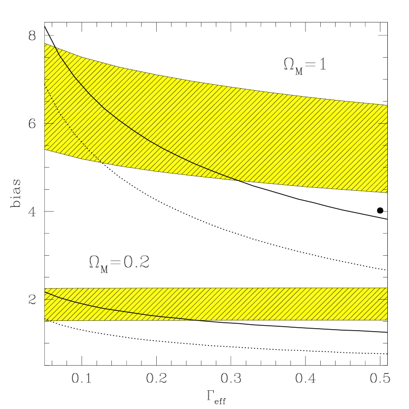
Figure 4: The spectrum-dependence of bias for objects of fixed abundance. Rarer (high-$\nu$) halos are more strongly clustered, but the details of the bias–abundance relationship depend upon the fluctuation power-spectrum. Spectra with more small scale power (higher $\Gamma$) have a lower bias for objects of given abundance. The solid curves show the predicted bias of dark halos as abundant as Lyman-break galaxies, and the dotted lines show the bias for halos ten times more abundant. Our 68% credible intervals on the bias are shaded. The results for $\Omega=0.3$ flat, discussed in the text, have been suppressed for clarity. The observations are consistent with all cosmologies considered ($\Omega_{M}=1$, $0.2$ open, $0.3$ flat) if the spectral shape $\Gamma$ is treated as a free parameter, though the preferred values $\Gamma\lower 2.15277pt\hbox{$\;\buildrel<\over{\sim}\;$}0.3$ arise more naturally if $\Omega_{M}<1$. Standard CDM, with $\Omega_{M}=1$ and $\Gamma=0.5$, seems to disagree with our data at about the $2\sigma$ level—but this is hardly the worst of its problems. The analytic approximations used are rather crude, and the point to the right of the plot, drawn from the $\Gamma=0.5,\Omega_{M}=1$ N-body simulation of Jing & Suto (1998), gives some idea of their reliability. The N-body estimate of the bias has been scaled to the values of $\sigma_{8}$ we adopt ($\sigma_{8}=0.5$ for $\Omega_{M}=1$, $\sigma_{8}=1$ for $\Omega_{M}=0.2$).

References

- (1)
- (2) Adelberger, K. L. et al. 1998, in preparation
- (3) Alcock, C. & Paczynski, B. 1979, Nature, 281, 358
- (4) Bagla, J. S. 1998, MNRAS, submitted
- (5) Bardeen, J. M., Bond, J. R., Kaiser, N., & Szalay, A.S. 1986, ApJ, 304, 15
- (6) Birnbaum, A. 1962, J. Am. Stat. Assn., 45, 164
- (7) Cole, S. & Kaiser, N. 1989, MNRAS, 237, 1127
- (8) Coles, P. & Jones, B. 1991, MNRAS, 248, 1
- (9) Coles, P. & Frenk, C. S. 1991, MNRAS, 253, 727
- (10) Dekel, A. & Rees, M. J. 1987, Nature, 326, 455
- (11) Eke, V. R., Cole, S., & Frenk, C. S. 1996, MNRAS, 282, 263
- (12) Giavalisco, M., Steidel, C. C., Adelberger, K. L., Dickinson, M. E., Pettini, M., & Kellogg, M. 1998a, ApJ, in press
- (13) Giavalisco, M. et al. 1998b, in preparation
- (14) Governato, F., Baugh, C. M., Frenk, C. S., Cole, S., Lacey, C. G., Quinn, T., & Stadel, J. 1998, Nature, in press
- (15) Jing, Y. P. & Suto, Y. 1998, ApJL, submitted
- (16) Kaiser, N. 1984, ApJL, 284, L9
- (17) Kaiser, N. 1987, MNRAS, 227, 1
- (18) Kofman, L., Bertschinger, E., Gelb, J., Nusser, A., & Dekel, A. 1994, ApJ, 420, 44
- (19) Maddox, S. J., Efstathiou, G., & Sutherland, W. J. 1996, MNRAS, 283, 1227
- (20) Mo, H. J., & White, S. D. M., 1996, MNRAS, 282, 347
- (21) Oke, J. B. et al. 1995, PASP 107, 3750
- (22) Padmanabhan, T. 1993, Structure Formation in the Universe (New York: Cambridge University Press)
- (23) Peacock, J. A., & Dodds, S. J. 1994, MNRAS, 267, 1020
- (24) Peacock, J. A. in The Most Distant Radio Galaxies: Proceedings of the KNAW colloquium (Amsterdam, Reidel), in press
- (25) Peebles, P. J. E. 1980, The Large Scale Structure of the Universe (Princeton: Princeton University Press)
- (26) Pettini, M., Kellogg, M., Steidel, C. C., Dickinson, M., Adelberger, K. L., & Giavalisco, M. 1998, ApJ, submitted
- (27) Press, W. H. & Schechter, P. 1974, ApJ, 187, 425
- (28) Steidel, C. C., Adelberger, K. L., Dickinson, M., Giavalisco, M., Pettini, M. & Kellogg, M. 1998a, ApJ, 492, 428
- (29) Steidel, C. C., Adelberger, K. L., Dickinson, M., Giavalisco, M., Pettini, M. & Kellogg, M. 1998b, in The Young Universe, eds. A. Fontana & S. d’Odorico (San Francisco: ASP), in press.
- (30) Steidel, C. C., Giavalisco, M., Pettini, M., Dickinson, M., & Adelberger, K. L. 1996, ApJ, 462, L17
- (31) Steidel, C. C., Pettini, M., & Hamilton, D. 1995, AJ, 110, 2519
- (32) Steidel, C. C., & Hamilton, D. 1993, AJ, 105, 2017
- (33) Vogeley, M. S., Park, C., Geller, M. J., & Huchra, J. P. 1992, ApJ, 391, L5
- (34) Wechsler, R. H., Gross, M. A. K., Primack, J. R., Blumenthal, G. R. & Dekel, A. 1998, ApJ, submitted
- (35) White, S. D. M., Efstathiou, G., and Frenk, C. S. 1993, MNRAS, 262, 1023
- (36) White, S. D. M. & Rees, M. J. 1978, MNRAS, 183, 341