Oscillation mode identifications and models for the $\delta$ Scuti star FG Virginis

Abstract

We present new spectroscopic and photometric time series observations of the $\delta$ Scuti star FG Vir. We detect the oscillations via changes in the equivalent widths of hydrogen and metal absorption lines. From the ratios between spectroscopic and photometric amplitudes, we assign $\ell$ values to the eight strongest oscillation modes. In particular, we identify two radial modes ($\ell=0$) and find that the main pulsation mode (147 $\mu$Hz) has $\ell=1$. One of the radial modes (at 140$\mu$Hz) is the fundamental, implying that two modes with lower frequencies are g-modes. For the radial modes, we compare frequencies with those calculated from a scaled $\delta$ Scuti star model and derive a density $0.1645\pm 0.0005\,\rho_{\odot}$. We then obtain a distance of $84\pm 3$ pc, in excellent agreement with the Hipparcos value. Finally, we suggest that a 3.5-day variability in all observables (equivalent widths and intensity) is caused by stellar rotation.

1 Introduction

Oscillations in multi-periodic variables such as $\delta$ Scuti, roAp and $\beta$ Cephei stars have been observed extensively during the past 20 years. But even with high-quality data, it is still extremely difficult to identify which modes are being detected. Kjeldsen et al. (kbvf95 (1995)) used a new technique to detect solar-like oscillations in the bright G sub-giant $\eta$ Boo through their effect on the equivalent widths of the Balmer lines. A subsequent discussion by Bedding et al. (bkrb96 (1996)) of the sensitivity of different observables to modes with different degree $\ell$ suggested that one can determine the $\ell$-value of a given mode by combining measurements of absorption-line equivalent widths with simultaneous photometric observations. To test this idea, we chose the bright and well-studied $\delta$ Scuti star FG Vir.

FG Vir (HD 106384; $V=6.57$) is a multi-periodic $\delta$ Scuti star. It has a main pulsation period close to 1.9 hours and shows a fairly complex oscillation spectrum. This star has been studied extensively during the last few years, resulting in the detection of at least 24 well-determined frequencies between 100 and 400 $\mu$Hz, with amplitudes from 0.8 to 22 milli-magnitudes (mmag; Breger et al. bhn95 (1995), br98 (1998)). Because of its slow rotation (which reduces the complicating effects of rotational splitting) and the large number of detected frequencies (some of which are probably g modes), FG Vir is one of the most promising candidates for performing asteroseismology on a $\delta$ Scuti variable. Observations and models of this star have been presented by Dawson et al. (dbl95 (1995)), Breger et al. (bhn95 (1995)) and Guzik & Bradley (gb95 (1995)).

By choosing a star like FG Vir we have the advantage of knowing the frequencies in advance. We are therefore able to determine the oscillation amplitudes and phases with high precision. The aim of this paper is to identify the $\ell$ values of the observed modes and to compare the oscillation frequencies with a pulsation model. A preliminary analysis of the observations presented in this paper was given by Viskum et al. (1997b ), while results on radial velocity measurements were given by Viskum et al. (1997a ).

2 Observations and basic data reduction

2.1 Spectroscopy

We obtained intermediate-resolution spectra of FG Vir using the DFOSC spectrograph mounted on the Danish 1.54-m at La Silla, Chile and the coudé spectrograph (B grating) on the 74-inch Telescope at Mt. Stromlo, Australia, during a period of more than two weeks in May 1996. A journal of the observations is given in Table 1. In total we obtained 652 spectra of FG Vir.

The DFOSC spectrograph was used in the echelle mode, covering a wavelength region from 4600Å to 8000Å at a resolution of $R\sim 4300$. Six echelle orders were recorded, each covering about 600Å and with an overlap between adjacent orders of about 370 Å. A S/N ratio of 250–360 was reached in the DFOSC data with a typical exposure time of 460 s. The S/N ratio was determined by measuring the standard deviation of the intensity of the normalized spectrum in two spectral windows free of absorption lines.

The Mt. Stromlo data consisted of single-order spectra, with a wavelength coverage of 6000Å to 7000Å. The dispersion was 0.49Å/pixel, with a resolution of about 1.5Å which was set by the slit width of 2 arcsec. The typical exposure time was 400 s.

Table 1: Journal of spectroscopic observations of FG Vir

Date	Site	HJD (start)	Length	No. of
UT		2450000 +	hours	spectra
1996 May 2	Stromlo	205.931	4.0	26
1996 May 3	Stromlo	206.834	4.2	31
1996 May 6	Stromlo	209.867	7.7	62
1996 May 7	Stromlo	210.838	5.9	47
1996 May 8	La Silla	212.484	6.2	34
1996 May 9	La Silla	213.486	6.3	45
1996 May 10	La Silla	214.496	6.1	43
1996 May 11	La Silla	215.496	6.0	50
1996 May 13	La Silla	216.550	4.7	27
1996 May 13	La Silla	217.492	6.0	41
1996 May 15	La Silla	218.525	5.1	40
1996 May 15	Stromlo	218.824	6.2	69
1996 May 15	La Silla	219.468	5.1	35
1996 May 17	La Silla	220.541	3.3	20
1996 May 17	La Silla	221.477	6.2	43
1996 May 18	La Silla	222.498	5.5	39

We used the IRAF package for bias subtraction, flat-field correction, extraction of the 1D spectra and subtraction of background scattered light. We found the Mt. Stromlo CCD to have a non-linearity of 7% from low-light levels to saturation, which we corrected in pre-processing. The DFOSC CCD camera was measured to be linear within 0.5% and no correction for non-linearities was performed.

The DFOSC spectra suffered from sky contamination and edge vignetting, which meant that the extracted spectra tapered from the centre to the edge. We therefore normalized the continuum by dividing each order by a curve containing the shape of the flat field. The Mt. Stromlo spectra did not suffer for this kind of edge vignetting, so a third order polynomial fit was used for the continuum normalization.

2.2 Photometry

We obtained Strömgren $uvby$-$\beta$ photoelectric photometry with the six-channel photometer mounted at the Danish 0.5-m reflector (SAT) at La Silla, Chile over 22 nights in 1996. Observations of FG Vir were interspersed with observations of the star HD 105912 (spectral type F5 V). This was used as a comparison star by Breger et al. (bhn95 (1995)), who found no variability. In Table 2 we present a journal of the observations. The precision per data point is about 3 mmag. During three of the nights, only the H$\beta$ index was obtained due to non-photometric weather conditions. A total of 768 useful data points (99 hours) were obtained.

To produce light curves from the raw data, we used a reduction program developed for the SAT telescope. The reduction included airmass correction using standard extinction coefficients and transformation to the standard instrumental system. Slowly varying effects were then removed by subtracting second-order polynomials for both FG Vir and the comparison star. Variations in FG Vir not due to oscillations were removed by subtracting the comparison star, resulting in the light curves whose analysis is described in Sec. 4.

Table 2: Journal of photometric observations of FG Vir

Date	HJD (start)	Filter	Length	No. of
UT	2450000 +		hours	data pts
1996 Apr 28	202.469	uvby-$\beta$	7.1	62
1996 May 1	205.470	uvby-$\beta$	6.9	69
1996 May 2	206.472	uvby-$\beta$	6.8	46
1996 May 3	207.465	uvby-$\beta$	7.2	48
1996 May 4	208.490	uvby-$\beta$	6.4	42
1996 May 5	209.469	$H{\beta}$	7.0	83
1996 May 7	210.511	$H{\beta}$	5.2	51
1996 May 8	212.464	uvby-$\beta$	6.9	46
1996 May 9	213.465	uvby-$\beta$	3.2	22
1996 May 10	214.457	uvby-$\beta$	7.3	48
1996 May 11	215.458	uvby-$\beta$	7.4	49
1996 May 13	217.462	uvby-$\beta$	7.2	45
1996 May 14	218.486	uvby-$\beta$	6.4	42
1996 May 15	219.470	$H{\beta}$	4.2	51
1996 May 17	221.461	uvby-$\beta$	6.4	43
1996 May 18	222.475	uvby-$\beta$	3.1	21

3 Determination of equivalent widths

Stellar acoustic oscillations ($p$ modes) can be measured via their effect on the equivalent widths (EWs) of the Balmer lines, which are sensitive to temperature. Metal lines are also sensitive to temperature changes (Bedding et al., bkrb96 (1996)), with the Fe i lines being particularly sensitive but in the opposite sense to the Balmer lines. We measured the equivalent widths of the metal lines by fitting profiles, but this technique was found unsuitable for the much stronger Balmer lines, for which we used a different method. Both techniques are described in the next sections.

3.1 Equivalent-width variations of the Balmer lines

As described by Bedding & Kjeldsen (bk98 (1998)), a robust way of estimating the EW of broad spectral lines involves a method analogous to Strömgren H${\beta}$ photometry. We have attempted several other methods, such as fitting directly to the line profile, without reaching the same internal precision.

Our adopted method involved calculating the flux (number of counts) in three software filters, one centred on the line ($L$) and the others on the continuum on the red ($C_{R}$) and the blue ($C_{B}$) sides of the line. For each spectrum, we first adjusted its slope so that the fluxes were equal in the continuum filters: $C_{R}=C_{B}=C$. We then calculated the quantity

$$W={(C-L)\over C}.$$ (1)

This calculation was repeated for a large number of positions around the line centre by moving the three filters together in wavelength by small amounts to find the position which maximized the value of $W$. The whole procedure was repeated for different filter widths, in a way analogous to aperture radii selection in CCD photometry, and the results combined to give an estimate of the equivalent width (see Bedding & Kjeldsen bk98 (1998) for more details).

Our La Silla spectra cover both the H$\alpha$ and H$\beta$ lines, while only H$\alpha$ is present in the Mt. Stromlo data. In Fig. 1a we present the amplitude spectrum of the H$\alpha$ EW for the combined data set (Mt. Stromlo and La Silla), where the amplitude is measured in promille (parts per thousand). All amplitude spectra in this paper were calculated using a weighted least-squares sine-wave fit to the time series (see Frandsen et al. kapboo (1995), 6134.camp (1996)). The pulsation signal is clearly seen in the range 100–400$\mu$Hz. Fig. 1b shows the residual spectrum obtained after subtracting 23 previously published frequencies (as described in Sec. 4). The mean noise level in the residual spectrum at high frequencies (600–800$\mu$Hz) is 0.18 promille, while it is 0.35 promille in the frequency range where the oscillation signal is found (100 – 400 $\mu$Hz). The S/N of the dominant peak at 147 $\mu$Hz is about 58.

Figure 1: (a) Amplitude spectrum of the oscillations in FG Vir measured through the EW of the H$\alpha$ line of the total data set (Mt. Stromlo and La Silla). The amplitude is measured in promille (parts per thousand). The inset shows the amplitude spectrum of the window function. (b) Residual spectrum after subtraction of 23 known oscillation frequencies.

Fig. 2 shows the amplitude spectrum of the EW measurements of the H$\beta$ line (La Silla only). The oscillations are again obvious, but the noise is more than a factor two higher than for H$\alpha$, due in part to bad CCD columns that could not be removed by bias subtraction or flat fielding.

Figure 2: Amplitude spectrum of the oscillations in FG Vir measured through the EW of the H$\beta$ line (La Silla data only).

3.2 Equivalent-width variations of metal lines

The spectra from La Silla consist of six echelle orders containing many metal lines. The line identifications, kindly provided by F. Kupka and M. Gelbmann, were made using the program described by Gelbmann (gelb95 (1995)) and Gelbmann et al. (gelb97 (1997)). We measured the EWs by fitting Gaussians to the line profiles, with the surrounding continua being fitted using low-order polynomials. The fitting was done iteratively using the Levenberg-Marquard method (Press et al. press (1989)) to estimate the line position, line depth and continuum level. A first estimate was made for these parameters over a narrow wavelength interval, and an improved continuum was calculated over a broader range of the spectrum. In addition to the EW, this also yielded other parameters to be used for decorrelation.

The time series of each line was decorrelated against external parameters. A detailed discussion of our decorrelation procedure can be found in Frandsen et al. (6134.camp (1996)). We used parameters that were derived either from the spectra or from the CCD frames and were known not to contain any information on the EWs or the pulsations. Any correlation between the measured EWs and these parameters must then have been due to a systematic effect and was corrected by subtracting a simple linear fit. The procedure was repeated until no significant correlations were present. This procedure increased the S/N significantly: for example, the improvement was a factor of 3.3 for the sum of all 20 lines described below.

From the EW measurements we detected the strongest pulsation period of FG Vir in all Fe i, Ca i and Mg i lines, with amplitudes from 7 and 22 promille. Noise levels in the amplitude spectra ranged from about 0.9 promille up to more than 3 promille for the weakest or highly blended lines.

We also examined lines of ionized elements, which are potentially useful for calibration. The reason is that in FG Vir, these lines are near their maximum strength as a function of temperature (Gray gray (1992)) and thus are expected to be stable with respect to variations in the temperature induced by the stellar pulsation. We indeed found these lines to have very low amplitudes in EW, with some of the Si ii lines having no detectable variability. For example, the Si ii line at 6372Å was stable in EW at the level of 2.7 promille (3$\sigma$). We used the EW of this line as a decorrelation parameter for the Fe i lines.

Table 3: Amplitude of the strongest oscillation mode in FG Vir as measured in EW for twenty strong Fe i lines.

$\lambda$	Line	depth	A147	$\sigma$(A147)
(Å)	ID	(%)	(promille)
4958	1-14	23	13.4	1.1
”	2-26	24	13.0	1.5
4983	2-25	14	18.5	1.2
5003	2-23	15	15.1	1.7
5041	1-19	15	13.1	1.2
”	2-21	16	16.1	2.1
5227	2-13	25	12.7	0.8
5270	2-28	21	12.4	0.9
5329	2-10	20	14.1	0.9
5341	3-25	20	13.4	0.9
5370	2-08	13	16.3	1.6
5404	3-22	10	20.2	1.8
5406	3-21	11	21.2	2.0
5424	3-19	11	9.6	2.0
5430	3-18	12	17.7	2.3
5456	2-04	11	6.8	3.0
”	3-15	13	9.0	2.0
5477∗	2-03	11	17.8	2.2
5616	3-05	11	15.1	1.7
5659	3-03	10	22.0	1.6

^∗this line is blended with a strong Ni i line.

The Fe i lines give the best opportunity for mode identification. Table 3 lists the 20 strongest unblended lines, where Column 1 is the central wavelength, Column 2 is our line ID number (the first digit indicates echelle order in which the line falls), Column 3 is the relative line depth (in percent), Column 4 is the amplitude of the strongest mode and Column 5 is the uncertainty in this amplitude. Three of the chosen Fe i lines are detected in two echelle orders. For these lines, the two measurements of oscillation amplitude agree within the errors. All the lines have the same phases within the uncertainties. As evident from Table 3, the amplitude of the main mode changes between the different lines. This could be due to variations in the temperature sensitivity of the different Fei lines, or due to blending with other species with different temperature sensitivities to Fe i.

Figure 3: Amplitude spectrum of twenty combined Fe i lines measured through the EW using profile fitting.

Fig. 3 shows the amplitude spectrum obtained by combining the EW time series of the twenty strong Fe i lines, weighted according to their signal-to-noise ratios. To be precise, the combined time series $w(t)$ was obtained from the 20 individual series $w_{i}(t)$ using the following equation

$$w(t)=\frac{\left(\sum\frac{w_{i}(t)}{A_{i}}\mbox{(S/N)}_{i}^{2}\right)\;\left(\sum A_{i}\;\mbox{(S/N)}_{i}^{2}\right)}{\left(\sum\mbox{(S/N)}_{i}^{2}\right)^{2}},$$ (2)

where $A_{i}$ is the amplitude of the 147 $\mu$Hz mode and $\mbox{S/N}_{i}=A_{i}/\sigma(A_{i})$ is its signal-to-noise ratio. The noise level in Fig. 3 is 0.5 promille in amplitude. Oscillations are present with sufficient signal-to-noise in this combined data set to allow the amplitudes to be used for mode identification. In the next section we measure amplitudes for as many modes as possible in each of the observables (EWs and photometry), to allow ratios to be calculated for mode identification.

4 Frequency Analysis

Our data set suffers from a poor window function, which produces very high side-lobes (see Fig. 1), which complicates the determination of frequencies in the Fourier domain. Fortunately, Breger et al. (bhn95 (1995), br98 (1998)) have determined very precise oscillation frequencies for FG Vir from data obtained over many years. We have therefore chosen to rely on these frequencies instead of trying to determine them from our data set.

First, however, we must check whether our data set is consistent with the main oscillation frequencies found by Breger et al. (bhn95 (1995), br98 (1998)). By pre-whitening with their frequencies, we found that the ten strongest pulsation modes of Breger et al. (bhn95 (1995)) are also present in our data set. From the residual spectrum it was clear that more modes are present at lower S/N.

Knowing the frequencies in advance reduces the task of determining amplitudes and phases to a linear problem. We used the program ISF (Frandsen et al. kapboo (1995)), which is a least-squares routine that simultaneously fits a series of known frequencies to a given time series. To maximize the precision, we have fitted all 23 frequencies determined by Breger et al. (br98 (1998)) to each time series, except one frequency ($f_{20}$) which is very close to an alias of one of the other frequencies. Table 4 lists the amplitudes for H$\alpha$, H$\beta$ and the combined Fe i spectral lines. We have used the same mode numbering as Breger et al. (br98 (1998)). Although all 23 frequencies were fitted, we shall only use the eight modes for which S/N$>5$ in both H$\alpha$ EW and photometry (see also Table 5). Fig. 1b shows the residual spectrum for H$\alpha$ EW after subtraction of the fit.

Table 4: Pulsation modes detected in different spectral lines measured via the EW

ID	Frequency		Amplitudes
			H$\alpha$ line	H$\beta$ line	Fe i lines
	$\mu$Hz	c/d	promille	promille	promille
$f_{1}$	147.18	12.716	20.3	20.2	14.1
$f_{2}$	280.42	24.228	3.9	3.0	3.1
$f_{3}$	270.87	23.403	3.9	3.4	4.0
$f_{4}$	243.65	21.052	3.2	3.3	1.5
$f_{5}$	229.95	19.868	3.1	2.3	1.4
$f_{6}$	140.67	12.154	3.7	3.6	4.0
$f_{7}$	111.76	9.656	4.1	4.3	1.9
$f_{8}$	106.47	9.199	3.0	4.0	1.6

Fig. 4 shows amplitude spectra (in mmag) for the fourStrömgren filters. The signal can clearly be seen in each filter, with the expected decrease in amplitude from blue to red. Eight frequencies are detected with S/N$>5$, with amplitudes given in Table 5. The same eight frequencies were detected in the $b-y$ index with lower S/N. In the $\beta$ index, only two frequencies could be found with adequate S/N but the table includes the amplitudes for all eight frequencies for completeness. The mean noise levels in the residual amplitude spectra of the $u$, $v$, $b$, $y$, $b-y$ and $\beta$ time series are 0.42, 0.42, 0.40, 0.35, 0.16 and 0.29 mmag, respectively. These were used to calculate the S/N values in Table 5.

Because the frequencies are known, the amplitudes can be estimated with better precision than would be expected from the above noise values. The formal solution gives standard deviations of the derived amplitudes for the uvby data to be 0.07 mmag. However, from tests made by determining amplitudes from subsets of the different time series, we find that the main uncertainty on the amplitudes comes from the very complicated window function. Furthermore, some of the modes are closely spaced in frequency and are not well separated in our data. This is especially true for the closest pair of modes $f_{2}=280.42\mu$Hz and $f_{11}=280.09\mu$Hz, which are unresolved by our observations. The derived amplitudes of these modes change when data are added to or removed from the time series. In order to minimize the influence of the window function on the amplitudes, so as to be able to compare amplitudes from different observables, we have removed a few nights from the photometric time series to obtain an observing window similar to that of the La Silla spectroscopic observations. In this way, even if amplitudes of some modes are slightly wrong due to the complicated window function, this effect should be about the same in each time series and therefore cancel when we calculate the amplitude ratios.

Breger et al. (bhn95 (1995)) presented broad-band $V$ photometry for the ten strongest modes in FG Vir, which we can compare with our Strömgren $y$ amplitudes. For the strongest mode ($f_{1}$) they obtained an amplitude of 22.0 mmag, which is in good agreement with our $y$ amplitude. We also agree on all other amplitudes, within the observing errors, except the $f_{3}$ mode at $270\mu$Hz, which has a much higher amplitude in our data set. As discussed by Breger et al. (br98 (1998)), the amplitude of the $f_{3}$ mode has been highly variable. It has increased from 1.4 mmag in 1992, 2.3 mmag in 1993 to 4.1 mmag in 1995, and our 1996 measurement gives 5.2 mmag.

Table 5: Strömgren photometry for FG Vir

ID	Freq.	Amplitudes
		$u$			$v$			$b$			$y$			$b-y$			$\beta$
	$\mu$Hz	mmag	S/N		mmag	S/N		mmag	S/N		mmag	S/N		mmag	S/N		mmag	S/N
$f_{1}$	147.18	32.5	77		32.4	77		27.6	69		22.0	63		5.4	33		5.3	18
$f_{2}$	280.42	6.5	15		6.5	15		6.5	16		5.7	16		1.2	7.3		0.7	2.5
$f_{3}$	270.87	7.1	17		7.3	17		6.5	16		5.2	15		1.0	6.5		1.3	4.4
$f_{4}$	243.65	4.6	11		4.5	11		4.2	10		3.6	10		0.7	4.2		1.2	4.0
$f_{5}$	229.95	3.3	7.8		3.3	7.8		2.8	7.0		2.6	7.5		0.4	2.5		0.5	1.8
$f_{6}$	140.67	7.8	18		7.6	18		6.0	15		5.3	15		0.8	5.1		1.0	3.4
$f_{7}$	111.76	5.3	12		5.2	12		5.0	13		4.3	12		0.6	4.0		0.9	3.1
$f_{8}$	106.47	3.9	9.3		4.3	10		3.5	8.8		3.0	8.6		0.5	3.3		0.8	2.8

Figure 4: Amplitude spectra in the four Strömgren filters

5 Mode identification

The investigation by Bedding et al. (bkrb96 (1996)) into the sensitivity of various observing methods to modes with different $\ell$ showed that the Balmer-line EWs have a spatial response similar to that of radial velocity measurements. This is because velocity measurements only detect the component along the line of sight to the star and so, when integrated over the stellar disk, are preferentially weighted to the central regions. Balmer lines have a strong centre-to-limb variation, becoming much weaker towards the limb, and therefore have a response to oscillations similar to that of radial velocities. Intensity measurements, on the other hand, give less spatial resolution because the centre-to-limb variation in intensity (‘limb darkening’) is relatively small. Bedding et al. went on to suggest that this difference in spatial response between simultaneous EW and intensity measurements could be used to determine the $\ell$ value of a mode.

They also investigated the temperature dependence of several other absorption lines (Fe i, Ca ii, G-band and Mg b feature) and found the Mg b feature and the Fe i lines to be especially useful for oscillation measurements. These spectral lines have much smaller centre-to-limb variations than the Balmer lines and so have spatial responses similar to that of intensity measurements. This means that mode identifications can be done with our observations by comparing Balmer EW amplitudes with either intensity amplitudes or Fe i EW amplitudes. Modes with different degree $\ell$ should occupy different locations in an amplitude-ratio diagram.

A preliminary analysis of our observations was given by Viskum et al. (1997b ), where only the ratio of Balmer-line EWs to intensity amplitudes was considered. In that paper, we found a clear grouping of the different modes in an amplitude-ratio diagram, and proposed a preliminary mode identification for the ten dominant frequencies. In this paper, we present a more thorough investigation of the different measurements, including the many Fe i lines present in our spectra.

Figure 5: Amplitude ratios (H$\alpha$/Intensity) versus (H$\alpha$/Fe i) of the eight dominant modes in FG Vir. The EW amplitudes are calculated from the total data set (Mt. Stromlo and La Silla). The intensity amplitudes are a mean of the four Strömgren filters ($uvby$). Labels show the mode frequencies in $\mu$Hz (truncated to integer values).

Fig. 5 shows the amplitude ratios (H$\alpha$/Fe i) versus (H$\alpha$/Intensity) for the eight dominant modes, obtained using the total H$\alpha$ data set (Mt. Stromlo and La Silla). Note that amplitudes of oscillations in EW are measured in promille, while photometric amplitudes are measured in mmag. The data points come from Tables 4 and 5, while the 1-$\sigma$ error bars are based on the tests on data subsets referred to in Sec. 4. The intensity amplitudes are the mean of the amplitudes in the four Strömgren filters (uvby), in order to improve the signal-to-noise. Only the eight dominant modes are shown because of the large uncertainties on the remaining modes.

The modes are clearly grouped into three regions. We identify the group at lower left as radial modes ($\ell=0$), followed by one dipole mode ($\ell=1$) and a group with $\ell\geq 2$. This trend follows the results of Bedding et al. (bkrb96 (1996)), who calculated that the amplitude ratio between different methods should become greater as $\ell$ increases. An important result from this diagram is that the Fe i lines indeed have spatial responses similar to that of intensity measurements, as predicted by Bedding et al. (bkrb96 (1996)), which shows that mode identification can be done from spectroscopic measurements alone. This is a very important result because it allows one to obtain a mode identification based on a single data set, with a common window function and frequency resolution.

Figure 6: Same as Fig. 5, but without the Mt. Stromlo H$\alpha$ data.

One problem arises immediately: two of the modes in the lower-left group ($f_{2}=280.42\,\mu$Hz and $f_{3}=270.87\,\mu$Hz) are too closely spaced in frequency for both to be radial modes. Fig. 6 shows the same amplitude ratios, except that the Mt. Stromlo H$\alpha$ data have been excluded. The separation of the modes is less clear. In particular, the $f_{2}$ mode has now moved away from the radial group towards the $\ell=1$ group. We ascribe this to the change in resolution between the different data sets, which re-distributes the power between the two unresolved modes discussed in Sec. 4 ($f_{2}$ and $f_{11}$). We have confirmed using simulations that, because of the presence of $f_{11}$, the amplitude ratio measured for the $f_{2}$ mode is very sensitive to the sampling and to their phase difference. We expect more reliable results when the Mt. Stromlo data are omitted because the spectroscopic data will then have a very similar window function to the photometric data. However, our simulations show that even the remaining small differences in the sampling, which inevitably arise from the differences in statistical weights, will produce systematic errors in the amplitude ratio. Of the modes identified by Breger et al. (bhn95 (1995)), the pair $f_{2}$ and $f_{11}$ have by far the smallest separation (0.32 $\mu$Hz). Of those for which we have EW data, the mode involved in the next closest separation is $f_{4}$, which is more than 2 $\mu$Hz from $f_{14}$. We therefore do not expect other modes in our figures to be affected to the same extent as $f_{2}$, and we see that they are not. We conclude that the mostly likely identification is $\ell=0$ for $f_{3}$ and $\ell=1$ for $f_{2}$.

Figure 7: Amplitude ratios (H$\beta$/Fe i) versus (H$\alpha$/Fe i) of the eight dominant modes with $1\sigma$ error bars. Only La Silla data

Fig. 7 shows the amplitude ratios (H$\beta$/Fe i) versus (H$\alpha$/Fe i). The diagram shows that the H$\alpha$ and the H$\beta$ lines have essentially the same spatial response to the oscillations. Together, the three amplitude-ratio diagrams indicate the sensitivity of different observables applied for mode identifications and the robustness of the method.

Table 6: Mode identifications for FG Vir

ID	Frequency		$\ell$-identification
	$\mu$Hz	c/d	Breger et al. (bhn95 (1995))	This work
$f_{1}$	147.18	12.72	0	1
$f_{2}$	280.42	24.24	0	1
$f_{3}$	270.87	23.41	2	0
$f_{4}$	243.65	21.06	1	2
$f_{5}$	229.95	19.87	2	2
$f_{6}$	140.67	12.16	21	0
$f_{7}$	111.76	9.66	21	21
$f_{8}$	106.47	9.20	21	21

¹ Possible $g$-mode.

The mode identifications are summarized in Table 6 and Fig. 8. In the table we also show the identifications given by Breger et al. (bhn95 (1995)) and as seen the agreement is poor. This identification set is actually only one of several possible solutions selected by Breger et al. (bhn95 (1995)) from a family of stellar models. They chose this solution, because it was in agreement with the constraints provided by the spectroscopic determination by Mantegazza et al. (mpb94 (1994)), who found the $f_{1}$ mode to be radial. At the same time Breger et al. (bhn95 (1995)) found from two-colour photometry a negative phase shift ($\phi_{B-V}-\phi_{V}=-10.4\pm 2^{\circ}$) for the primary frequency ($f_{1}$). This actually excludes the possibility of $f_{1}$ being a radial mode, and indeed, this is also the result we obtain from the amplitude ratio diagrams. Moreover, recent work by Breger et al. (br97comm (1997)) agrees with our identifications for all eight modes in Table 6. The earlier disagreement clearly demonstrates the difficulty of classifying modes by using comparisons between stellar models and observed frequencies, without the help of additional information.

Our identification of the strongest mode as dipole ($\ell=1$) is in good agreement with this mode’s photometric negative phase difference obtained by Dawson et al. (dbl95 (1995)). Another important result is that, as we show below, the $f_{6}$ mode is probably the fundamental radial mode ($n=1$, $\ell=0$)). In this case, the two modes with lower frequencies ($f_{7}$ and $f_{8}$) must be $g$-modes. These modes will be particular interesting for asteroseismology because they contain information about the convective core and convective overshooting.

The above interpretation is based on the results obtained by Bedding et al. (bkrb96 (1996)), who considered the special case in which the rotation axis points towards the observer, so that contributions only arise from zonal modes ($m=0$). Different orientations of the axis and the influence of non-zero $m$ values on the amplitude-ratio diagrams need to be investigated in detail. However, provided the dependence of amplitudes on $m$ is smaller than the dependence on $\ell$, our identifications are likely to be correct.

Figure 8: Schematic diagram of the eight strongest modes in FG Vir, with our $\ell$-identifications. The vertical axis shows the photometric amplitude in Strömgren $y$.

6 Comparison with a pulsation model

6.1 Density of FG Vir

Once the oscillation modes are identified, the next step in a seismic analysis is to compare the observed frequencies with models. Calculating a full theoretical model for FG Vir is beyond the scope of this paper. However, much progress can be made by scaling from existing model calculations. Here we use calculations by Christensen-Dalsgaard (cd93 (1993)) for a $2.2M_{\odot}$ star with solar metallicity, generated during investigations of the $\delta$ Scuti variable $\kappa^{2}$ Bootis (Frandsen et al. kapboo (1995)). Our aim is to make an accurate estimate of the mean density of FG Vir using the radial modes. We do this by using a model that is homologous to FG Vir.

Two stars are homologous if their mass distributions are related by a simple spatial scaling factor (Kippenhahn & Weigert kw (1990)). That is, suppose the two stars have masses $M$ and $M^{\prime}$ and radii $R$ and $R^{\prime}$, and the mass enclosed by radius $r$ (or $r^{\prime}$) is $m$ (or $m^{\prime}$). Then at all points where the relative radii are equal ($r/R=r^{\prime}/R^{\prime}$), the relative enclosed masses will also be equal ($m/M=m^{\prime}/M^{\prime}$). This being the case, and assuming the stars have the same chemical composition, the oscillation frequencies of one star can be found by multiplying the frequencies of the other star by a constant (equal to the square root of the ratio of their densities).

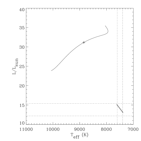
Figure 9: H–R diagram showing the evolutionary track of the 2.2 $M_{\odot}$ model. The cross marks the model most closely homologous to FG Vir (see Sec. 6.1). The vertical dotted lines show the 1-sigma range in $T_{\rm eff}$ for FG Vir measured by Mantegazza et al (mpb94 (1994)). The horizontal dotted lines show the 1-sigma range in luminosity determined from the Hipparcos distance (see Sec. 6.2). The pair of diagonal lines are contours of constant density and define the $\pm 3\sigma$ asteroseismic solution given in Table 7.

Figure 10: Theoretical frequencies of the radial oscillation modes of a 2.2 $M_{\odot}$ star with solar metallicity ($Z=0.02$), plotted as a function of stellar density (the star evolves from right to left). The dotted lines show the frequencies of the two observed modes in FG Vir that we have identified as radial.

The evolutionary track of the 2.2 $M_{\odot}$ model is shown in Fig. 9. The model is calculated from the zero-age main sequence (ZAMS) until the end of the core hydrogen-burning phase. Fig. 10 shows the frequencies of the radial modes of the 2.2$M_{\odot}$ model, plotted as a function of stellar density. As the model star evolves from right to left, the density and the frequencies both decrease. We only consider radial modes because those of higher degree have more complicated time dependencies (Christensen-Dalsgaard cd93 (1993); Frandsen et al. kapboo (1995)). The horizontal dotted lines indicate the two observed modes in FG Vir that we have identified as radial ($f_{3}$ and $f_{6}$). Since the mass of FG Vir is somewhat less than 2.2 $M_{\odot}$, as we shall see, our aim is not to find an exact match to the model frequencies. Instead, we locate the stage in the evolution of the model at which the structure of the model is homologous to that of FG Vir. This will occur when the model frequencies and those of FG Vir are related by a single multiplicative factor (which will be the square root of the density ratio). The first step is therefore to identify a pair of radial modes in the model which match the observed frequency ratio ($f_{3}/f_{6}=1.926$).

Figure 11: Frequency ratios for the radial modes of the 2.2 $M_{\odot}$ model. The star evolves from right to left. The horizontal dotted line shows the ratio between the two modes in FG Vir that we have identified as radial. The vertical dotted lines shows the density of the corresponding model ($0.203\,\rho_{\odot}$). That model should be homologous to FG Vir.

Fig. 11 shows frequency ratios for the radial modes of the 2.2 $M_{\odot}$ model. We see that only one pair of modes matches the observed frequency ratio, which leads us to identify $f_{6}$ with $n=1$ and $f_{3}$ with $n=4$. The density of the corresponding 2.2 $M_{\odot}$ model is $0.203\,\rho_{\odot}$ and we select this as the model most closely homologous to FG Vir. To estimate the density of FG Vir, we simply multiply the density of the homologous model ($0.203\,\rho_{\odot}$) by the square of the ratio $f_{\rm obs}/f_{\rm model}$. The result is $0.164\,\rho_{\odot}$.

We note in passing that the identification of $f_{2}=280.42\,\mu$Hz as a radial mode (see Sec. 5) is inconsistent with the model frequencies. It is clear from Fig. 11 that the ratio $f_{2}/f_{6}=1.993$ does not match the frequency ratio for any of the models.

We can now attempt to identify other radial modes among the published frequencies. Based on the above densities, the radial mode with $n=2$ should have a frequency of 185.8 $\mu$Hz. Breger et al. (br98 (1998)) observed a mode at 186.04 $\mu$Hz ($f_{12}$) which is a good match. An exact fit to this observed frequency requires a density for FG Vir of $0.1647\rho_{\odot}$. This differs from the above value by 0.3%, providing an idea of the uncertainty in this process. It seems likely that $f_{12}$ is a radial mode, but its amplitude is too weak for spectroscopic confirmation.

Using the same argument, the radial mode with $n=3$ should have a frequency of 228.6 $\mu$Hz. The two observed frequencies nearest this value are $f_{5}=229.95$ $\mu$Hz and $f_{9}=222.55$ $\mu$Hz (Breger et al. br98 (1998)). The best match is $f_{5}$ but the discrepancy is 0.6% (1.2% in density) and our amplitude-ratio diagrams indicate that this mode is not radial. The frequency $f_{9}$ differs from the expected value by 2.7% and we have no information about its $\ell$ value. We therefore do not identify either of these as the radial $n=3$ mode.

Figure 12: Scaled density for FG Vir versus model density. For each radial mode, as a function of model density, we plot model density multiplied by $(f_{\rm obs}/f_{\rm model})^{2}$. The model most closely homologous to FG Vir has a density of about $0.203\,\rho_{\odot}$ (vertical dotted line). The derived density for FG Vir, shown by the horizontal dotted lines, is $0.1645\pm 0.0005\,\rho_{\odot}$.

To further establish the uncertainty in our density estimate, we have constructed the plot in Fig. 12 as follows. For each of the three observed radial modes, we take each time step in the model evolution and use the ratio $(f_{\rm obs}/f_{\rm model})^{2}$ to calculate the density that FG Vir would have if it were homologous to the model at that time step. This scaled density is plotted as a function of the model density. We see that the scaled density is fairly insensitive to exactly which stage in the model evolution is chosen. In other words, although the model most closely homologous to FG Vir has a density of $0.203\,\rho_{\odot}$ (vertical dotted line in Fig. 12), adjacent models do quite well (note the scales on the axes differ by more than a factor of 20). Indeed, the model with the same actual density as FG Vir has similar absolute frequencies to FG Vir (to better than 0.5%), indicating that even this model is a reasonably good representation of FG Vir.

On the basis of this discussion, we can set limits on the density of FG Vir as shown by the horizontal dotted lines in Fig. 12, which are chosen to span the three density estimates. We then have:

$$\rho=0.1645\pm 0.0005\,\rho_{\odot}.$$ (3)

That is, assuming solar metallicity for FG Vir, we have determined the density to a precision of about 0.3%. It would clearly be desirable to obtain a spectroscopic measurement of the metallicity of this star, since this will affect the density at the level of about 1%.

6.2 Distance and mass of FG Vir

The effective temperature of FG Vir was determined spectroscopically by Mantegazza et al. (mpb94 (1994)) to be $7500\pm 100$ K. From the models used in the seismic analysis of $\kappa^{2}$ Boo (Frandsen et al. kapboo (1995)), we have derived a relationship between luminosity, mass and effective temperature for stars with this effective temperature. For solar metallicity ($Z=0.02$) we find

$${L\over L_{\odot}}\simeq 0.99\left({M\over M_{\odot}}\right)^{4.8}\left({T_{\rm eff}\over 5777\mbox{ K}}\right)^{-0.8}$$ (4)

Since $L\propto R^{2}T_{\rm eff}^{4}$ and mean density is proportional to $M/R^{3}$, we then have:

$${\rho\over\rho_{\odot}}\simeq 1.0021\left({T_{\rm eff}\over 5777\mbox{ K}}\right)\left({R\over R_{\odot}}\right)^{-2.5833}$$ (5)

Table 7: Parameters of FG Vir for three different values of temperature

$T_{\rm eff}$	7400 K	7500 K	7600 K
$R/R_{\odot}$	2.215 $\pm$ 0.003	2.227 $\pm$ 0.003	2.238 $\pm$ 0.003
$L/L_{\odot}$	13.21 $\pm$ 0.03	14.08 $\pm$ 0.03	15.00 $\pm$ 0.03
$M/M_{\odot}$	1.788 $\pm$ 0.008	1.816 $\pm$ 0.008	1.844 $\pm$ 0.008
$\log g^{a}$	3.999 $\pm$ 0.001	4.002 $\pm$ 0.001	4.004 $\pm$ 0.001

^a units of $g$ are cm s^-2

Using the density given in Equation 3, we can then estimate the radius, luminosity and mass of FG Vir. Table 7 shows the results for three values of effective temperature. The quoted uncertainties only include the uncertainty in the mean density. The values in Table 7 define a locus of constant density in the H–R diagram, as shown in Fig. 9. The portion of this curve that lies between the extremes of valid temperatures defines the solution.

Table 8: Parameters of FG Vir based on asteroseismic density^a

$\rho/\rho_{\odot}$	0.1645 $\pm$ 0.0005
$R/R_{\odot}$	2.227 $\pm$ 0.012
$L/L_{\odot}$	14.1 $\pm$ 0.9
$M/M_{\odot}$	1.82 $\pm$ 0.03
$\log g$	4.002 $\pm$ 0.003
distance (pc)b	84 $\pm$ 3

^a assuming $T_{\rm eff}=7500\pm 100$ K and $Z=0.02$.
^b using $L/L_{\odot}$, $V=6.57$, $BC=-0.07$ and $M_{\rm bol,\odot}=4.75$.

The main sources of uncertainty in this process arise from imprecise knowledge of the temperature and metallicity and from the use of the relation between $L$, $M$ and $T_{\rm eff}$ (Equations 4 and 5). Assuming that the main uncertainty is the temperature, we find the properties of FG Vir listed in Table 8. The errors are not independent: increasing the temperature will increase the luminosity, mass and radius.

The derived distance is in excellent agreement with the Hipparcos value of $83\pm 5$ pc, as is also clear from Fig. 9. It is important to note that if the temperature had been better known, e.g. to $\pm 30$ K, we would have obtained an error on the distance of only $\pm 1\mbox{ pc}$ (internal error). The surface gravity agrees with the value of $\log g=3.9\pm 0.2$ determined spectroscopically by Mantegazza et al. (mpb94 (1994)). The high precision of our $\log g$ determination arises because $g$ is given by $\rho R$.

Table 9: Parameters of FG Vir based on Hipparcos distance^a

distance (pc)	83 $\pm$ 5
$L/L_{\odot}$b	13.8 $\pm$ 1.6
$R/R_{\odot}$	2.20 $\pm$ 0.15
$M/M_{\odot}$	1.82 $\pm$ 0.03
$\rho/\rho_{\odot}$	0.17 $\pm$ 0.03
$\log g$	4.0 $\pm$ 0.05

^a assuming $T_{\rm eff}=7500\pm 100$ K and $Z=0.02$.
^b using distance, $V=6.57$, $BC=-0.07$ and $M_{\rm bol,\odot}=4.75$.

Table 9 shows the fundamental properties for FG Vir obtained by combining the Hipparcos distance with Equations 4 and 5, without using the asteroseismically determined density. It can be seen that the asteroseismic properties for FG Vir are far more precise than those obtained by using the Hipparcos data, even with 100 K uncertainty in the temperature. Such calculations show clearly the potential of asteroseismology. The present analysis is based on three $\ell=0$ modes out of more than 20 known frequencies. We have identified modes with $\ell=1$ and $\ell=2$ and these modes will contain accurate information on the detailed evolutionary stage of FG Vir. This should provide strong constraints on models computed specifically for FG Vir, resulting in a fine-tuned model. The effect from metallicity should also be investigated.

To check our identification of $\ell=0$ modes, we compared all 24 frequencies published by Breger et al. (br98 (1998)) with the frequency ratios of radial modes in the 2.2M_⊙ model. The highest correlation occurred with the following solution: $f_{6}$ ($n=1$), $f_{12}$ ($n=2$), $f_{5}$ ($n=3$) and $f_{3}$ ($n=4$), with a scatter between observed and best-fit theoretical frequencies of about 1 $\mu$Hz. These identifications are in full agreement with our own results and give us confidence that we have correctly identified the radial modes in FG Vir.

Finally, we note that the strongest mode ($f_{1}$) is likely to be $n=1$, $\ell=1$ and is probably undergoing an avoided crossing with a $g$-mode. This would make this mode very interesting for testing a more detailed model.

7 Rotation period of FG Vir

A periodic trend was evident in the raw EW data for all metal lines and in the two Balmer lines. The same periodicity was seen in all four photometric light curves. The variation is clearly seen after removal of the known pulsation signal and smoothing (Fig. 13).

Figure 13: The raw time series for (a) the photometric light curve in the $u$ filter; (b) the H$\alpha$ line EW (small symbols: Mt. Stromlo data, large symbols: La Silla data); (c) the combined Fe i EW time series. The dotted curve shows a damped oscillation with a period of 3.5 days and with a mean lifetime (the inverse of the damping constant) of 14 days.

There appears to be a variability with a period of $3.5\pm 0.2$ days and a decaying amplitude. Note that the H$\alpha$ time series is composed of data from telescopes at two different sites, while the Fe i and H$\alpha$ time series were obtained using different reduction programs. Furthermore, the photometric time series were obtained with a third telescope. All time series are in phase, indicating that the variation is caused by the same phenomenon.

We propose that this 3.5-day variation is intrinsic to the star and reflects the rotation period of FG Vir. Using the asteroseismic radius in Table 8, we then obtain $v_{eq}=33\pm 2$ km s^-1 for the equatorial velocity. Using the value of $v\sin i=21\pm 1$ km s^-1 found by Mantegazza et al. (mpb94 (1994)) gives $i=40\degr\pm 4\degr$ for the inclination angle, in agreement with the value of $i=31\degr\pm 5\degr$ found by Mantegazza et al. from a moments analysis of $f_{5}$ and $f_{7}$.

8 Summary of results

We have investigated a new technique to measure the oscillations in $\delta$ Scuti stars via changes in the equivalent widths of absorption lines. An important advantage of this new technique is that only medium-dispersion spectra are needed, which makes the method suitable for small and medium-sized telescopes and for multi-site campaigns. Our main results are summarized below.

• Our detection of oscillations in FG Vir from equivalent-width measurements of H$\alpha$, H$\beta$ and Fe i lines is an important confirmation of the method developed by Kjeldsen et al. (kbvf95 (1995)) to search for solar-like oscillations.

• From the ratios between oscillation amplitudes measured in EW and the four Strömgren filters (uvby), we have identified $\ell$-values for eight modes in FG Vir.

• We suggest that the two lowest-frequency modes are g-modes, while the strongest mode (147.2$\mu$Hz) is a dipole mode.

• By comparing the frequencies of radial modes with model calculations, we obtained a precise density and derived a distance that is in excellent agreement with the Hipparcos value.

• We detected a long-period variation in the time series with a period of 3.5 days, which we propose is caused by rotation of the star.