Search for star clustering: methodology and application to the Two Micron Galactic Survey

Abstract

A new approach to the study of the large-scale stellar cluster distribution in the Galaxy based on two-point correlation techniques is presented. The basic formalism for this method is outlined and its applications are then investigated by the use of a simple model of cluster distribution in the Galaxy. This provides an estimate of the potentials of the two-point correlation function for indicating clustering in the measured star positions, which can be related to the presence of star clusters in the observed field. This technique is then applied to several areas of the Two Micron Galactic Survey catalogue, from which information is obtained on the distribution of clusters according to position in the Galaxy, as well as about age, density of stars, etc.

1 Introduction

Open star clusters provide valuable information on the evolution of the Galaxy. In this paper two-point correlation techniques are used to analyse the distribution of open clusters in order to gain an insight into the structure and evolution of the Galaxy.

Open-cluster distributions have been widely studied at optical wavelengths as a means of studying Galactic structure and evolution (see, for example, Lyngå 1987b; Janes & Phelps 1994). The Lyngå catalogue of open clusters (Lyngå 1987a) lists about 1200 clusters, which represent nearly all the open clusters accessible in the visible. Knowledge of the positions and ages of these clusters (a method of age determination for clusters is given by Carraro & Chiosi 1994) enables the scale length and scale height of the disc to be derived for both young and old clusters (for a review of old open clusters, see Friel 1995) and theories to be developed on their formation and destruction throughout the history of the Galaxy.

The limitations on these studies are imposed by the maximum distance at which open clusters can be detected. Most of the cataloged open clusters are in the solar neighbourhood, and very few have distances greater than 3 kpc (Payne-Gaposchkin 1979). Hence, information is obtained only for a small region of the Milky Way. The problem is caused by interstellar extinction. An excellent tool for studying star clusters and star formation regions is to observe in the infrared (Wynn-Williams 1977), where the effect of the extinction is far less. To date, however, the infrared has been little used in this field owing the absence of suitable databases.

The $K$ band is probably the best region of the spectrum for tracing the stellar distribution of the Galaxy. The $K$ radiation is a mass tracer in spiral galaxies because it follows the old stellar population (Rhoads 1995). Furthermore, the $K$ light is dominated by high-mass stars in star formation regions, i.e. in open clusters, so it is especially appropriate in the search for young clusters, which are rich in massive stars.

As explained in more detail by Garzón et al. (1993), the Two micron Galactic survey (TMGS) is a $K$-band survey of various regions along the Galactic equator between $-5^{o}<l<35^{o}$, $|b|\leq 15^{\circ}$ and $35^{\circ}<l<180^{\circ}$, $|b|\leq 5^{\circ}$. The TMGS catalogue has a positional accuracy of about 4 arcsec in right ascension and 7 arcsec in declination. These errors have been estimated after cross-correlating the original TMGS source positions with Guide Star Catalogue (GSC) counterparts. The larger error in declination comes from the orientation of the array with respect to the survey direction. Due to the dead spaces between detectors, the $K$ limiting magnitude for completeness has to be set conservatively within a range from 9 to 9.5 mag, although the detection limit magnitude of the survey is well in excess of 10 mag.

In this paper a new method is presented for automatically determining the level of clustering in catalogues, the TMGS being used as an example. A set of criteria are defined for an automatic search for correlations among stars by means of the two-point correlation function and the two-point angular correlation function. A simple model which assumes a regular distribution of clusters with a constant star density is developed in Section 3. Predictions from this model are then compared with the TMGS and the discrepancies analysed. The causes of clustering are then discussed. The use of the tools described in Section 2 and their application to the TMGS catalogue are dealt with in Section 5, and the results for several regions of our Galaxy are given in Section 6. Finally, a summary of the results is given, and suggestions are made for future developments of the methodology described here.

2 The two-point correlation function and the two-point angular correlation function

Occasionally, when the scale length of a system is changed, certain aspects of the system remain invariable, as in the case for the distribution of matter in space. For example, there are mathematical methods for handling the spatial distribution of atoms in solids, gases and (particularly) liquids. Cosmologists face the same kind of mathematical problem when working with the distribution of galaxies and clusters of galaxies in the context of the large-scale structure of the Universe. They treat the Universe as a fluid whose ‘particles’ are galaxies. Our aim in this paper is to develop the use of similar mathematical methods on an intermediate scale, i.e. in examining the distribution of the stars that make up our Galaxy.

Correlation functions describe how points are distributed (e.g. Peebles 1980; Borgani 1995). Suppose a local density of objects $\delta N/{\delta V}=\rho(\vec{r})$ and an average density $\langle\rho\rangle$ (hereafter, the symbol $\langle\cdots\rangle$ indicates a local volume average). Note that $\rho$ corresponds to the exact distribution of objects, i.e. it is a Dirac delta function with zero value where there are no objects, and $\langle\rho\rangle$ is the local average density, i.e. the number of objects per unit volume, and provides no information concerning their distribution.

The two-point correlation function (TPCF) is defined as

$$\xi(|\vec{r}-\vec{r}^{\prime}|)=\frac{\langle\rho(\vec{r})\rho(\vec{r}^{\prime})\rangle}{\langle\rho(\vec{r})\rangle^{2}}-1.$$ (1)

The function $\xi(r)$ expresses the excess over the random probability of finding objects at separation $r$. ($\xi(r)=0$ means that the probability is totally random; $\xi(r)>0$ that the probability is greater than random, i.e. that there is clustering; and $\xi(r)<0$ that the probability is less than random, i.e. that there is relative avoidance).

In the same way, the two-point correlation function can be defined for two dimensions on the surface on to which the distribution is projected (the celestial sphere in the case considered here). This is called the two-point angular correlation function (TPACF) and is defined as

$$\omega(|\vec{\theta}-\vec{\theta}^{\prime}|)=\frac{\langle\sigma(\vec{\theta})\sigma(\vec{\theta}^{\prime})\rangle}{\langle\sigma(\vec{\theta})\rangle^{2}}-1,$$ (2)

where $\sigma$ is the surface density per unit solid angle.

Another mathematical technique for deciding whether a distribution is non-Poissonian is area tessellation, as was used by Balázs (1995) to test the grouping tendency of H_α-emission stars in the Orion molecular clouds without giving a quantitative measure of the departure from the Poissonian distribution. See also Pásztor et al. (1993), Pásztor & Tóth (1995) and references therein for other astronomical applications of spatial statistics.

2.1 Relationship between the TPCF and the TPACF for stars

When applying the above definitions to stars in the Galaxy, the luminosity function and space density have to be taken into account.

By generalizing the result of the Limber (1953) equation for constant density, the relationship between the TPCF (which is non-zero for distances less than $\Delta r$) and the TPACF (for small $\theta$) for any density distribution is

$$\omega_{\rm t}(\theta)\approx\frac{1}{\langle\sigma_{\rm t}\rangle^{2}}\int_{0}^{\infty}dr\ r^{4}\langle\rho\rangle^{2}(r)\int_{r-\Delta r}^{r+\Delta r}dr^{\prime}$$

$$\times\int_{M_{\rm min}(r)}^{M_{\rm max}(r)}dM\ \phi(M)\int_{M_{\rm min}(r)}^{M_{\rm max}(r)}dM^{\prime}\ \phi(M^{\prime})$$

$$\times\xi\left(\sqrt{(r\theta)^{2}+(r-r^{\prime})^{2}};r,M,M^{\prime}\right),$$ (3)

where $r$ is the distance along the line of sight, $M$ the absolute magnitude, $\phi(M)$ the luminosity function and

$$\langle\sigma_{\rm t}\rangle=\int_{0}^{\infty}dr\ r^{2}\langle\rho\rangle(r)\int_{M_{\rm min}(r)}^{M_{\rm max}(r)}dM\ \phi(M).$$ (4)

The minimum and maximum values of $M$ for a distance $r$ depend on the minimum and maximum values of the apparent magnitude and the extinction along the line of sight.

In this case, it is assumed that the absorption is not patchy, i.e. that it is independent of $\theta$ for small angles. This is not exactly true but it will be show in Section 2.4 that the effects are negligible.

The subscript ‘t’ stands for ‘total’, a projection of all distances and magnitudes, and $\langle\sigma_{\rm t}\rangle$ is the total two-dimensional density for all distances and magnitudes. In the literature, $\langle\sigma_{\rm t}\rangle$ is also called $A(m_{\rm min},m_{\rm max},l,b)$ and represents the star counts in the magnitude range (Bahcall 1986).

This expression enables the TPACF to be found once the three-dimensional distribution of the stars is known and forms the basis of this article, in which we create a model distribution of the stars and compare the results obtained with those observationally in order to investigate the distribution of clustering in the structure of our Galaxy.

In general, the TPACF cannot be inverted to give the TPCF due to the multiplicity of possible solutions and to the lack of precise knowledge of certain parameters. However, there are certain cases in which the equation can be inverted and TPCF obtained from TPACF (Fall & Tremaine 1977). A trivial example where inversion is possible is that of a Poissonian three-dimensional distribution, which implies a Poissonian projected distribution and vice versa, i.e. $\xi=0$, $\omega=0$ on all scales. Another example is when $\langle\rho\rangle(r)$ is a constant independent of $r$.

2.2 Definition of new variables

In order to simplify the comparison of the level of clustering for different regions of the sky, two new variables will be introduced.

$\theta_{\rm max}$ is defined as the first zero of $\omega_{\rm t}(\theta)$. In this article (see for example Fig. 7), $\omega_{\rm t}$ is positive up to a separation $\theta_{\rm max}$. For values greater than $\theta_{\rm max}$ this value is small and oscillates about zero, as there is no correlation among stars separated by large angular distances.

Another definition, corresponding to the integration of $\omega_{\rm t}$ up to the limit $\theta=\theta_{\rm max}$ ($\theta>\theta_{\rm max}$ would give a null contribution to the integral), is

$$C_{2}\equiv\frac{\int_{0}^{\theta_{\rm max}}d\theta\ \theta\omega_{\rm t}(\theta)}{\theta_{\rm max}^{2}},$$ (5)

which means the excess (when $C_{2}$ is positive) or deficit (when $C_{2}$ is negative) of the relative number of objects with respect to a Poissonian distribution in a circle centred on an arbitrary star on the celestial sphere, within the observed solid angle and with angular radius $\theta_{\rm max}$. The relative correlation within the angular scale $\theta_{\rm max}$ is therefore measured. We call $C_{2}$ the ‘accumulation parameter’ (N.B. there are also other definitions in the literature of the TPACF integral, e.g. Wiedemann & Atmanspacher 1990).

The variable $C_{2}$ has a clear meaning associated with projected clustering and is also a useful number to measure. Since it sums several values of $\omega$ for different angles, it condenses the information of interest into a single number that can be compared for different samples of stars and give the degree of clustering. This parameter is a mathematical expression of the degree of clustering seen in fields of stars. The idea that we wish to stress here is that all mathematical developments described in this paper are designed to put the intuitive idea of clustering to a reliable test. These calculations are necessary for a quantitative, as opposed to a merely qualitative, description of clustering.

Applying the expression (3) of $\omega_{\rm t}$ in $C_{2}$, we get

$$C_{2}=\frac{1}{\langle\sigma_{\rm t}\rangle^{2}\theta_{\rm max}^{2}}\int_{0}^{\infty}dr\ r^{2}\langle\rho(r)\rangle^{2}\int_{M_{\rm min}(r)}^{M_{\rm max}(r)}dM\ \phi(M)$$

$$\times\int_{M_{\rm min}(r)}^{M_{\rm max}(r)}dM^{\prime}\ \phi(M^{\prime})\int_{0}^{\theta_{\rm max}r}dy\ y\Xi(y;r,M,M^{\prime}),$$ (6)

where $\Xi$, an integrated TPCF, is

$$\Xi(y;r,M,M^{\prime})$$

$$=\int_{r-\Delta r}^{r+\Delta r}dr^{\prime}\xi\left(\sqrt{y^{2}+(r-r^{\prime})^{2}};r,M,M^{\prime}\right).$$ (7)

2.3 Further approximations

In order to simplify the above calculations, it will be assumed that the distribution of stars does not depend on their luminosity, i.e. that $\xi(y;r,M,M^{\prime})=\xi(y;r)$. This is not completely true as there is a small dependence on the distribution of stars in a cluster according their masses, and the luminosities are dependent on the masses. A complete calculation taking the luminosity function into consideration would be of great value. However, the relationship between the TPCF and the luminosity function is uncertain, although the effects of this approximation for the detection of clusters are expected to be small.

With this approximation, and from (4) and (3),

$$\langle\sigma_{\rm t}\rangle=\int_{0}^{\infty}dr\ \langle N^{*}\rangle(r)$$ (8)

and

$$\omega_{\rm t}(\theta)=\frac{1}{\langle\sigma_{\rm t}\rangle^{2}}\int_{0}^{\infty}dr\ \langle N^{*}\rangle^{2}(r)\Xi(r\theta;r),$$ (9)

where $\langle N^{*}(r)\rangle$ is the number of stars observed per unit solid angle at a distance $r$:

$$\langle N^{*}\rangle(r)=r^{2}\langle\rho\rangle(r)\int_{M_{\rm min}(r)}^{M_{\rm max}(r)}dM\ \phi(M).$$ (10)

The variable $\omega_{\rm t}$ can also be expressed as

$$\omega_{\rm t}(\theta)=\overline{\Xi(\overline{r}\theta)}$$ (11)

where the averages $\overline{r}$ and $\overline{\Xi}$ are such that match (9).

Also, from (6),

$$C_{2}=\frac{1}{\langle\sigma_{\rm t}\rangle^{2}\theta_{\rm max}^{2}}\int_{0}^{\infty}dr\ \frac{\langle N^{*}(r)\rangle^{2}}{r^{2}}\int_{0}^{\theta_{\rm max}r}dy\ y\Xi(y;r).$$ (12)

This last equivalence is a way of averaging the function $\xi$.

Hence, high values of $C_{2}$ indicate that there must be high projected clustering in the direction of the beam.

2.4 Patchiness of extinction

It is clear that extinction can distort the observed counts, the amount of the distortion being a matter of controversy. It is generally accepted that in the optical wavelengths this influence is very severe, particularly in regions near to or in the Galactic plane in the inner Galaxy, where the strong and patchily distributed obscuration makes it difficult to penetrate deep into the Galaxy. The amount of extinction decreases substantially with increasing wavelength. Maihara et al. (1978) quoted a value of 0.17 mag kpc^-1 as typical for extinction in the Galactic plane in the $K$ band, compared with 1.9 mag kpc^-1 for the $V$ band (Allen 1973).

This has two important consequences. First, the $K$ band is more effective at penetrating the interstellar dust. Secondly, the observed stellar distribution more closely resembles the true distribution. For the second argument to be true it is necessary that the obscuration in the $K$ band should not only be smaller in amount than in the $V$ band, but also that its patchiness should be less important.

This rather uniform distribution of the interstellar extinction in $K$ can be inferred from the TMGS histograms in several cuts across the Galactic plane. Garzón et al. (1993, their Fig. 8) compared the observed stellar distribution in the TMGS and the GSC in the $V$ band. It is noticeable how uniform the $K$ histograms are, particularly when compared with those for the GSC. Except for small portions highly concentrated in the Galactic plane and more marked in the central regions, the shape of the high spatial resolution distribution curves of the TMGS does not exhibit the ‘noisy’ pattern of the GSC plots, which is certainly due to the presence of strong and patchily distributed extinction.

Hammersley et al. (1994) showed similar histograms for different areas which also have similar shapes. Moreover, a good fit to a classical exponential disc can be seen in Fig. 3 of that paper; this would not be the case if the extinction were important and non-uniform.

This conclusion can also be reached from the contour maps of the bulge of the Galaxy of Dwek et al (1995), who showed the residuals of the DIRBE data after disc subtraction and extinction correction. Again, the general shape of the maps proves the basic uniformity of extinction distribution in the near infrared.

We now estimate these effects. From (4) with the change of variable $r=10^{(5+m_{\rm max}-M_{\rm max})/5}$ and

$$\Phi(M_{\rm max})=\int_{-\infty}^{M_{\rm max}}dM\ \phi(M)\approx\int_{M_{\rm min}}^{M_{\rm max}}dM\ \phi(M),$$ (13)

the local cumulative counts $\sigma_{\rm t}$ follow the expression

$$\sigma_{\rm t}=\langle\sigma_{\rm t}\rangle_{local}=200(\ln\ 10)10^{3m_{\rm max}/5}\omega\int_{-\infty}^{\infty}dM_{\rm max}$$

$$\times D\left(10^{(5+m_{\rm max}-M_{\rm max})/5}\right)10^{-3M_{\rm max}/5}\Phi(M_{\rm max}),$$ (14)

ignoring the variation of extinction with the distance. If we take the density $D$ as constant, then

$$\sigma_{\rm t}=N(m_{\rm max})\propto 10^{3m_{\rm max}/5}.$$ (15)

Taking $D$ as constant is sufficient for estimating the the order of magnitude of the patchiness due to extinction. In any case, the above proportionality is followed in the observed cumulative counts but with a constant value of between 1 and 2 instead of $3/5$ in the exponent.

An excess of extinction, $\Delta a(\theta)$, due for example to a cloud at an angular distance $|\vec{\theta}-\vec{\theta_{0}}|$ with respect to a given point $\theta_{0}$, will cause a reduction in the apparent flux of a fraction, $f$, of stars (behind the cloud), thereby creating the same effect as a reduction in the maximum apparent magnitudes of these stars by $\Delta a(\theta)$ mag, or, if $\Delta a(\theta)$ is relatively small, a reduction in $m_{\rm max}$ by $f\Delta a(\theta)$ mag for all stars. Hence,

$$\sigma_{\rm t}(\theta)\sim\sigma_{\rm t}(\theta_{0})10^{-3(a(\theta)-a(\theta_{0}))f/5}.$$ (16)

If it is assumed that the observed flux fluctuations, $\Delta F$, are due mainly to extinction variations, with the small-fluctuation approximation, then both are related by

$$\Delta a=-2.5\log\left(1-\frac{1}{f}\frac{\Delta F}{F}\right)\approx\frac{5\log_{10}e}{2f}\frac{\Delta F}{F}$$ (17)

(the factor $f$ appears again here for the same reasons as above). So, from equation (16), using the small-fluctuation approximation,

$$\frac{\sigma_{\rm t}(\theta)}{\sigma_{\rm t}(\theta_{0})}\sim\frac{3}{2}\frac{F(\theta)}{F(\theta_{0})}.$$ (18)

This means that the angular correlation of star density is about 3/2 times the angular correlation of the flux.

Averaging the DIRBE $K$ flux (Boggess et al. 1992) fluctuations from the maps with $2520^{\prime\prime}$ resolution over $\mid b\mid\leq 3^{\circ}$ for constant-$l$ strips over the range $-35^{\circ}<l<35^{\circ}$ (where the effects of extinction are most relevant), we get root mean squares of

$$0.03<\sigma(\Delta F/F)_{l={\rm const.},\mid b\mid\leq 3^{\circ}}<0.23,$$ (19)

with an average of

$$\overline{\sigma(\Delta F/F)_{l={\rm const.},\mid b\mid\leq 3^{\circ}}}=0.10.$$ (20)

The oscillations of flux fluctuations are not very high in the plane, their maximum being $2.3$ times the average.

From equation (18), and taking into account that the root mean square is $\sqrt{\omega(0)}$,

$$\overline{\omega(0)_{l={\rm const.},\mid b\mid\leq 3^{\circ}}}\sim 0.015$$ (21)

for regions of 2520^′′ in size. In the most unfavourable case, where the extinction is highest (multiplied by a factor of 2.3² because the maximum root mean square is $2.3$ times greater than the average), $\omega(0)\sim 0.08$.

Higher-resolution flux maps are not available in the $K$-band for the whole sky so we cannot derive these numbers for smaller scales, but they are not expected to be much higher since average cloud size is of the order of degrees (rather higher than 42^′) and the cloud distribution is fairly smooth. A fractal distribution would increase the contamination but this may apply only to very cold gas clouds (Pfenninger & Combes 1994) which are not the main cause of extinction in the $K$ band.

We conclude that extinction in $K$ cannot be responsible for correlations $\omega(0)$ greater than $\sim 0.08$. This is just an estimate, but the order of magnitude should not be very different. As will be shown, the results when applied to the TMGS are above this value (see, for example, Fig. 7), and causes other than patchy extinction must explain this.

3 A simple clustering model

In order to gain an understanding of how the accumulation parameter ($C_{2}$) varies with Galactic position, a model of stellar distribution is required. The model to be adopted in this section is very simple and consists of a group of spherical star clusters separated by distances much larger than the sizes of the clusters and embedded in a Poissonian distribution of field stars with average density $\rho_{\rm nc}$ . The density of clusters is $\langle n_{\rm cl}\rangle$. To simplify the problem, a constant star density, $\rho_{\rm cl}$, is assumed for each cluster ($\rho_{\rm nc}<\rho_{\rm cl}$); it is also assumed that the clusters have the same radius, $R_{\rm cl}$ (i.e. they are filled homogeneous spheres). In fact, the density of clusters, their radii and their internal stellar densities are different in different regions of the Galaxy, however there is insufficient information to construct a more detailed model, and our main interest here is in how $C_{2}$ varies qualitatively.

According to the definition, the TPCF is the average of the product of two numbers (for a distance $y$): the first is the probability of finding an object in a given position, and the second is the number of times that the object counts in a shell of radius between $r$ and $r+dr$ exceeds the same counts in a Poissonian distribution. The first number, the probability of finding an object in a volume $dV$ centered on $\vec{r}$ within a total volume $V$, is $\rho(\vec{r})dV/\langle\rho\rangle V$. With regard to the second number (Fig. 1), there are two cases to be considered:

Figure 1: Intersection of two spheres.

1. When $\vec{r}$ is at distance $x<R_{\rm cl}+y$ from the centre of a cluster, the second number is the sum of the excess (with respect the average, i.e. $\langle\rho\rangle$) of objects in the part of the shell that is inside the cluster ($S_{\rm ss}(x;y,R_{\rm cl})/4\pi y^{2}\times(\rho_{\rm cl}-\langle\rho\rangle)/\langle\rho\rangle$) minus the deficit of objects in the part of the shell outside the cluster ($(4\pi y^{2}-S_{\rm ss}(x;y,R_{\rm cl}))/4\pi y^{2}\times(\langle\rho\rangle-\rho_{\rm nc})/\langle\rho\rangle$). Here $S_{\rm ss}(x;y,R_{\rm cl})$ is the area of a spherical surface of radius $y$ inside another sphere of radius $R_{\rm cl}$ whose centre is at distance $x$ from the first one.

2. When the distance, $x$, from any cluster is larger than $R_{\rm cl}+y$, the second number is the negative quantity $-(\langle\rho\rangle-\rho_{\rm nc})/\langle\rho\rangle$, i.e. the deficit of objects compared with a Poissonian distribution with density $\langle\rho\rangle$.

When $y$ is sufficiently large there will be cases in which the shell intersects more than one cluster. However, such large values of $y$ are of no interest here, and only those cases in which the magnitude of $y$ is of the same order as that of $R_{\rm cl}$ will be considered.

Thus, the expression for the TPCF is

$$\xi(y)=\langle n_{\rm cl}\rangle 4\pi\int_{0}^{R_{\rm cl}}dx\ x^{2}\frac{\rho_{\rm cl}}{\langle\rho\rangle}$$

$$\times\left[\frac{S_{\rm ss}(x;y,R_{c}l)(\rho_{\rm cl}-\langle\rho\rangle)-(4\pi y^{2}-S_{\rm ss}(x;y,R_{\rm cl}))(\langle\rho\rangle-\rho_{\rm nc})}{4\pi y^{2}\langle\rho\rangle}\right]$$

$$+\langle n_{\rm cl}\rangle 4\pi\int_{R_{\rm cl}}^{R_{\rm cl}+y}dx\ x^{2}\frac{\rho_{\rm nc}}{\langle\rho\rangle}$$

$$\times\left[\frac{S_{\rm ss}(x;y,R_{c}l)(\rho_{\rm cl}-\langle\rho\rangle)-(4\pi y^{2}-S_{\rm ss}(x;y,R_{\rm cl}))(\langle\rho\rangle-\rho_{\rm nc})}{4\pi y^{2}\langle\rho\rangle}\right]$$

$$-\left[1-\langle n_{\rm cl}\rangle\frac{4}{3}\pi(R_{\rm cl}+y)^{3}\right]\frac{\rho_{\rm nc}}{\langle\rho\rangle}\left(\frac{\langle\rho\rangle-\rho_{\rm nc}}{\langle\rho\rangle}\right).$$ (22)

The average density is

$$\langle\rho\rangle=\frac{4}{3}\pi R_{\rm cl}^{3}\langle n_{\rm cl}\rangle\rho_{\rm cl}+\left(1-\frac{4}{3}\pi R_{\rm cl}^{3}\langle n_{\rm cl}\rangle\right)\rho_{\rm nc},$$ (23)

so

$$\frac{\rho_{\rm nc}}{\langle\rho\rangle}=\frac{1-\frac{\rho_{\rm cl}}{\langle\rho\rangle}\frac{4}{3}\pi R_{\rm cl}^{3}\langle n_{\rm cl}\rangle}{1-\frac{4}{3}\pi R_{\rm cl}^{3}\langle n_{\rm cl}\rangle},$$ (24)

$$\frac{\rho_{\rm cl}-\rho_{\rm nc}}{\langle\rho\rangle}=\frac{\frac{\rho_{\rm cl}}{\langle\rho\rangle}-1}{1-\frac{4}{3}\pi R_{\rm cl}^{3}\langle n_{\rm cl}\rangle}$$ (25)

and

$$\frac{\langle\rho\rangle-\rho_{\rm nc}}{\langle\rho\rangle}=\frac{4}{3}\pi R_{\rm cl}^{3}\langle n_{\rm cl}\rangle\frac{\frac{\rho_{\rm cl}}{\langle\rho\rangle}-1}{1-\frac{4}{3}\pi R_{\rm cl}^{3}\langle n_{\rm cl}\rangle}.$$ (26)

Also, from the appendix A1:

$$\int_{0}^{R_{\rm cl}}dx\ x^{2}S_{\rm ss}(x;y,R_{\rm cl})$$

$$=\left\{\begin{array}[]{ll}\frac{4}{3}\pi R_{\rm cl}^{3}y^{2}\left(1-\frac{3}{4}\frac{y}{R_{\rm cl}}+\frac{1}{16}\left(\frac{y}{R_{\rm cl}}\right)^{3}\right),&\mbox{ $y<2R_{\rm cl}$}\\ 0,&\mbox{ $y\geq 2R_{\rm cl}$}\end{array}\right\}$$ (27)

and

$$\int_{R_{\rm cl}}^{R_{\rm cl}+y}dx\ x^{2}S_{\rm ss}(x;y,R_{\rm cl})$$

$$=\left\{\begin{array}[]{ll}\frac{4}{3}\pi R_{\rm cl}^{3}y^{2}\left(\frac{3}{4}\frac{y}{R_{\rm cl}}-\frac{1}{16}\left(\frac{y}{R_{\rm cl}}\right)^{3}\right),&\mbox{ $y<2R_{\rm cl}$}\\ \frac{4}{3}\pi R_{\rm cl}^{3}y^{2},&\mbox{ $y\geq 2R_{\rm cl}$}\\ \end{array}\right\}.$$ (28)

We insert the last five equalities in (22) and, after simplifying, this leads to:

$$\xi(y)=\left\{\begin{array}[]{ll}\langle n_{\rm cl}\rangle\left(\frac{\rho_{\rm cl}-\rho_{\rm nc}}{\langle\rho\rangle}\right)^{2}\frac{4}{3}\pi R_{\rm cl}^{3}\\ \times\left(1-\frac{4}{3}\pi R_{\rm cl}^{3}\langle n_{\rm cl}\rangle-\frac{3}{4}\frac{y}{R_{\rm cl}}+\frac{1}{16}\left(\frac{y}{R_{\rm cl}}\right)^{3}\right),&\mbox{$y<2R_{\rm cl}$}\\ -\langle n_{\rm cl}\rangle\left(\frac{\rho_{\rm cl}-\rho_{\rm nc}}{\langle\rho\rangle}\right)^{2}\frac{4}{3}\pi R_{\rm cl}^{3}\left(\frac{4}{3}\pi R_{\rm cl}^{3}\langle n_{\rm cl}\rangle\right),&\mbox{$y\geq 2R_{\rm cl}$}\\ \end{array}\right\}$$ (29)

The reader should bear in mind that the applicable value of $y$ which is that for distances smaller than the minimum distance between two clusters. Due to the properties of the TPCF, the quantity $\int_{\rm all\ space}dV_{y}\xi(y)=4\pi\int_{0}^{\infty}dy\ y^{2}\xi(y)$ should be equal to zero. This is not exactly the case in (29), which is not valid for $y$ as large as the typical distances among clusters. Nevertheless, it can be seen that $\int_{V_{y}=\langle n_{\rm cl}\rangle^{-1}}dV_{y}\xi(y)=0$, i.e. the volume in which (29) can be used is roughly $\langle n_{\rm cl}\rangle^{-1}$.

The behaviour of the function can be seen in the Fig. 2 for $\langle n_{\rm cl}\rangle R_{\rm cl}^{3}=10^{-3}$, $\rho_{\rm cl}/\rho_{\rm nc}=100$. It becomes constant for $y>2R_{\rm cl}$, and the value in which $\xi=0$ is $y=1.90R_{\rm cl}$, which also is very close to $2R_{\rm cl}$. In what follows, the term $\frac{4}{3}\pi R_{\rm cl}^{3}\langle n_{\rm cl}\rangle$ will be neglected because in practice it is too small (the separation among clusters is much larger than $R_{\rm cl}$).

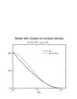
Figure 2: Two-point correlation function, $\xi$, and integrated two-point correlation function, $\Xi$, for a simple model.

The next step is the calculation of the integrated TPCF ($\Xi$) using (7) and including (29). In this case, $\Delta r$ is the first value that follows $\xi(\sqrt{y^{2}+(r-r^{\prime})^{2}})=0$, which is $\Delta r=\sqrt{4R_{\rm cl}^{2}-y^{2}}$. Hence,

$$\Xi\left(t=\frac{y}{2R_{\rm cl}}\right)=\int_{r-\sqrt{4R_{\rm cl}^{2}-y^{2}}}^{r+\sqrt{4R_{\rm cl}^{2}-y^{2}}}dr^{\prime}\xi(\sqrt{y^{2}+(r-r^{\prime})^{2}})$$

$$=\langle n_{\rm cl}\rangle\left(\frac{\rho_{\rm cl}-\rho_{\rm nc}}{\langle\rho\rangle}\right)^{2}\frac{4}{3}\pi R_{\rm cl}^{3}4R_{\rm cl}$$

$$\times\left[\sqrt{1-t^{2}}\left(\frac{3}{8}+\frac{3}{16}t^{2}\right)+\ln\left(\frac{\sqrt{1-t^{2}}+1}{t}\right)\left(\frac{-3}{4}t^{2}+\frac{3}{16}t^{4}\right)\right].$$ (30)

Fig. 2 shows that the behaviour of the TPCF and the integrated TCPF ($\xi$ and $\Xi$) are not very different.

Now, using (6), the observed value $C_{2}$ will be calculated. The theoretical lower limit of the integral should be zero, but in practice values under a $y_{\rm min}=r\theta_{\rm min}$ cannot be observed, due to the resolution $\theta_{\rm min}$ of our detector ($r$ is the distance of the zone of clusters).

$$\frac{1}{r^{2}\theta_{\rm max}^{2}}\int_{r\theta_{\rm min}}^{r\theta_{\rm max}}dyy\Xi(y)$$

$$=\left(\frac{2R_{\rm cl}}{r\theta_{\rm max}}\right)^{2}\langle n_{\rm cl}\rangle\left(\frac{\rho_{\rm cl}-\rho_{\rm nc}}{\langle\rho\rangle}\right)^{2}$$

$$\times\frac{4}{3}\pi R_{\rm cl}^{3}\left[\frac{1}{6}\ R_{\rm cl}\left(F\left(\frac{r\theta_{\rm min}}{2R_{\rm cl}}\right)-F\left(\frac{r\theta_{\rm max}}{2R_{\rm cl}}\right)\right)\right],$$ (31)

where $F(t_{0})$ is

$$F(t_{0})=24\int_{t_{0}}^{1}dt\ t$$

$$\times\left[\sqrt{1-t^{2}}\left(\frac{3}{8}+\frac{3}{16}t^{2}\right)+\ln\left(\frac{\sqrt{1-t^{2}}+1}{t}\right)\left(\frac{-3}{4}t^{2}+\frac{3}{16}t^{4}\right)\right]$$ (32)

($F(0)=1$, $F(1)=0$).

The observational value of $C_{2}$ would be an average of this quantity with weight $\langle N^{*}\rangle^{2}(r)$, according to (12), and with the characteristic parameters of the cluster depending on $r$, i.e. $\langle n_{\rm cl}\rangle(r)$ and $\left((\rho_{\rm cl}-\rho_{\rm nc})/\langle\rho\rangle\right)^{2}(r)$.

3.1 The contribution of a single shell of clusters

In the case where there are clusters only in the shell between $r$ and $r+\delta r$, with $\delta r/r\ll 1$, and where the contribution to $C_{2}$ is given only for this range of $r$ (when in the other ranges of $r$ the contribution is nil, or when the other shell with clusters has a negligible $\langle N^{*}\rangle(r)$), then

$$r\theta_{\rm max}\approx 2R_{\rm cl},$$ (33)

because the TPCF ($\xi$) in (29) is zero for this value (as $\frac{4}{3}\pi R_{\rm cl}^{3}\langle n_{\rm cl}\rangle$ is much smaller than unity). Then, introducing (33) in (31) and feeding the result into (12), we obtain

$$C_{2}=\frac{\langle N^{*}\rangle^{2}(r)\delta r}{\langle\sigma_{\rm t}\rangle^{2}}\langle n_{\rm cl}\rangle\left(\frac{\rho_{\rm cl}-\rho_{\rm nc}}{\langle\rho\rangle}\right)^{2}\frac{4}{3}\pi R_{\rm cl}^{3}$$

$$\times\left[\frac{1}{6}\ R_{\rm cl}F\left(\frac{\theta_{\rm min}}{\theta_{\rm max}}\right)\right].$$ (34)

The factor $F$ reduces the value of $C_{2}$ when $\theta_{\rm max}$ is only few times greater than $\theta_{\rm min}$. Since $\theta_{\rm max}=2R_{\rm cl}/r$, the more distant the clusters the smaller the value obtained for $C_{2}$. $\theta_{\rm max}$ is normally enough large compared with $\theta_{\rm min}$ for $F$ to be considered as always close to unity. The values that $F$ takes are shown in Table LABEL:Tab:F.

Table 1: Correction factor $F$ due to the finite resolution of the detector.

$x$	$F(x)$
0	1.000000
0.1	0.956356
0.2	0.838143
0.3	0.671930
0.4	0.487970
0.5	0.314330
0.6	0.172488
0.7	0.074429
0.8	0.021008
0.9	0.002144
$\geq 1$	0

As can be seen, when $x$ is greater than $\approx 1/4$, i.e. when the distance of the cluster is greater than $\sim R_{\rm cl}/2\theta_{\rm min}$, the effect of the factor $F$ begins to be noticeable.

3.2 Clusters distributed throughout the Galaxy

Suppose that there are clusters distributed throughout the Galaxy, i.e. that there are clusters at all distances along the line of sight in any direction. The TPACF ($\omega_{\rm t}$), which is related to the TPCF ($\xi$) through (9), is computed numerically. The function $\xi(y)$ is obtained with (29), where it is assumed that the size and star density in the cluster is the same in all clusters, and that also the density of clusters, $\langle n_{\rm cl}\rangle$, is proportional to the mean density of stars:

$$\langle n_{\rm cl}\rangle=C\langle\rho\rangle.$$ (35)

The density of stars ($\rho_{\rm nc}$) is inferred from the relationship (24). $\langle N^{*}\rangle(r)$ is calculated using (10), where $\langle\rho\rangle$ and $\phi(M)$ are calculated for a model Galaxy with two components: a disc and a bulge. The disc is taken from the Wainscoat et al. (1992) model and the bulge model described in López-Corredoira et al. (1997). The extinction law given in Wainscoat et al. (1992) is also used.

The explicit dependence of $C_{2}$ on $l$ and $b$ is calculated from the $\omega$ values and a $\theta_{\rm max}$ that is derived with the approximation $\theta_{\rm max}\approx 2R_{\rm cl}/\overline{r}$, where

$$\overline{r}=\frac{\int_{0}^{\infty}dr\ rN^{*}(r)}{\int_{0}^{\infty}dr\ N^{*}(r)}.$$ (36)

$\theta_{\rm max}$ is calculated in this way because the first zero of the function $\omega$ cannot be derived. In the previous approximations, $\omega$ was always positive and negative values were neglected .

When these operations are carried out for the values $R_{\rm cl}=1$ pc, $\rho_{\rm cl}=500\ pc^{-3}$ and $C=10^{-5}$, the results shown in Figures 3 and 4 are obtained.

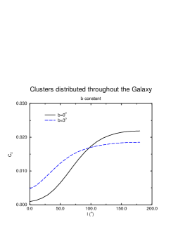
Figure 3: $C_{2}$ at $b=0^{\circ}$, $b=3^{\circ}$ and $b=10^{\circ}$ according to a distribution of simple clusters over all the Galaxy.

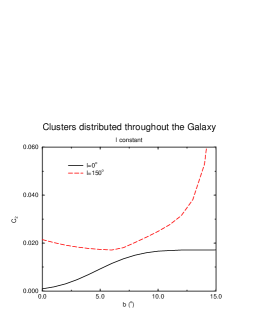
Figure 4: $C_{2}$ for different Galactic latitudes for $l=0^{\circ}$ and $l=150^{\circ}$ according to a distribution of simple clusters over all the Galaxy.

In Figures 3 and 4 it can be seen how the correlation increases with distance from the Galactic plane (increasing $|b|$) as well as with distance from the centre of the Galaxy (increasing $|l|$). An explanation of this can be seen directly in the expression (29), which is proportional to $\langle n_{\rm cl}\rangle\left((\rho_{\rm cl}-\rho_{\rm nc})/\langle\rho\rangle\right)^{2}$, where $\rho_{\rm cl}$ is a much larger constant than $\rho_{\rm nc}$ and $\langle n_{\rm cl}\rangle$ is proportional to $\langle\rho\rangle$. It can be seen that $\xi$ is greater for smaller values of $\langle\rho\rangle$, i.e. it is greater away from the Galactic plane and far away from the bulge. Since the angular correlation function is an average of all the correlation functions in the line of sight, it produces the above results.

This is merely a hypothetical example, and no meaning should be given to the actual values obtained since the parameters are invented. However, the qualitative dependence of $\omega$ on $l$ and $b$ is significant. This result is even more general than the particular case of the proportionality $\langle n_{\rm cl}\rangle=C\langle\rho\rangle$. An increase in $\omega$ for increasing $|l|$ or $|b|$ is given when $\langle n_{\rm cl}\rangle\left(({\rho_{\rm cl}-\rho_{\rm nc})/\langle\rho\rangle}\right)^{2}$ increases in a typical region in the line of sight. Even a dependence such as $\langle n_{\rm cl}\rangle=C\langle\rho\rangle^{\alpha}$ with $\alpha<2$ is acceptable to allow this kind of dependence. Another significant prediction is that in the anticentre region the dependence with $l$ is very smooth and nearly constant.

4 The causes of the clustering

The existence of clustering indicates that the formation of the stellar components of a cluster share the same time and place of birth, and that all the stars that are observed in the cluster once belonged to same originating cloud, which explains why they occupy a neighbouring position in space. The alternative hypothesis of an initial Poissonian distribution of stars which collapsed to form the cluster is not feasible because cluster’s gravity would have been too weak to restrain the velocities of the stars, which would have “evaporated” from the primitive cluster. The fact is, then, that clusters originate from earlier clusters that were formed from a cloud, or several clouds in the same region.

It is assumed in the TPCAF, equation (3), that only $\xi$, and not the extinction through the relationship between apparent magnitudes and absolute magnitudes, is dependent on $\theta$. As discussed in section 2.4, the contribution from cloud irregularity is irrelevant.

4.1 Relationship with the evolution time

The relationship of the accumulative parameter with the evolution time comes from the rate of evaporation of stars.

When the effects of dust clouds are ignored, all contributions to $C_{2}$ come from $\xi$, i.e. clusters that happen to be in the line of sight. The relationship with the evolution time is through $\rho_{\rm cl}$ since stars escape from the cluster over time. According to Chandrasekhar (1942), the rate of escape of stars is

$$\frac{\Delta\rho_{\rm cl}(t)}{\rho_{\rm cl}}\approx-Q\frac{\Delta t}{T_{\rm E}},$$ (37)

where $Q$ and $T_{\rm E}$ are constants that depend on the characteristics of the cluster. $Q$ is the rate of stars which can escape and $T_{\rm E}$ is the average time that takes these stars to leave the cluster. $Q$ is the fraction of stars with velocities greater than escape velocity. Chandrasekhar (1942) calculates a value of $Q=0.0074$ for a relaxed cluster. $T_{\rm E}$ (in Gyr) is the relaxation time that is, for an average cluster with $N$ stars, radius $R$ (in pc) and average stellar mass $\overline{m}$ (in $M_{\odot}$)

$$T_{\rm E}=8.8\times 10^{-4}\sqrt{NR^{3}/\overline{m}}\frac{1}{\log_{10}N-0.45}.$$ (38)

Insofar as $C_{2}$ is proportional to $\left((\rho_{\rm cl}-\rho_{\rm nc})/\langle\rho\rangle\right)^{2}$ through the proportionality dependence with $\xi$ in (29) and assuming $\langle n_{\rm cl}\rangle$ and $R_{\rm cl}$ as constant and $\rho_{\rm cl}\gg\langle\rho\rangle$, then $C_{2}$ may be approximated as

$$C_{2}(t)=C_{2}(t=0)e^{-\frac{Qt}{2T_{\rm E}}},$$ (39)

or, expressed differently,

$$C_{2}(t)=K_{1}\times e^{-t/K_{2}},$$ (40)

where $K_{1}$ and $K_{2}$ are positive constants.

This is the theory for simple cases but some cases are more complicated. Certain other effects are not negligible, such as dynamical friction (see Chandrasekhar 1943a,b,c) or Galactic rotation and gravitational tides (Wielen & Fuchs 1988), both of which produce different values of these constants. Spitzer (1958) points out that most open clusters should be destroyed by interactions with molecular clouds on time-scales of few hundred million years, meaning that few very old open clusters are known to have survived to the current epoch. However, $N$-body simulations (Terlevich 1987) predict that only by encounters with the most massive molecular clouds would the cluster be disrupted.

Apart from theoretical considerations, exponential decrease is indicated by other authors from observational data (for example, Lyngå 1987a). Janes & Phelps (1994) fit a relationship between the age and cluster abundance in the solar neighbourhood which follows a sum of two exponentials. If it is assumed that there is a constant creation of clusters, and that the death of a cluster corresponds to a low value of $\xi$, this would then imply that $C_{2}$ is dependent on the sum of two decaying exponentials, although with so many effects it is difficult to determine which is the correct dependence. What is clear, however, is that high values of $C_{2}$ indicate the existence of young clusters.

5 Measurement of correlations in the TMGS and other surveys

5.1 Measurement of the TPACF

The following discussion concerns the measurement of the TPACF derived from a rectangular field image of angular size $a\times b$ in a direction containing $N$ stars of known coordinates and magnitudes (between $m_{\rm min}$ and $m_{\rm max}$).

One method of determining correlation functions in a distribution of objects, discussed by Rivolo (1986), is to use the following estimator for $N$ points:

$$\langle\rho\rho\rangle(r)=\frac{\langle\rho\rangle}{N}\sum_{i=1}^{N}\frac{M_{i}(r)}{V_{i}(r)},$$ (41)

where $M_{i}(r)$ is the number of particles lying in a shell of thickness $\delta r$ from the $i$th particle, and $V_{i}(r)$ is the volume of the shell. The same applies to $\langle\sigma\sigma\rangle$ but with areas instead of volumes:

$$\langle\sigma\sigma\rangle(\theta)=\frac{\langle\sigma\rangle}{N}\sum_{i=1}^{N}\frac{M_{i}(\theta)}{\Omega_{i}(\theta)}.$$ (42)

This expression must be corrected for edge effects, i.e. some stars are lost in the calculation of $M_{i}(\theta)$ when a star $i$ is at distance less than $\theta$ from an edge of the rectangular image. In the quantity $\sum_{i=1}^{N}M_{i}(\theta)$, the excess probability is measured of finding a star at an angular distance $\theta$ from other stars in a ring of thickness $\Delta\theta$ with surface area $\Omega(\theta)$ and this should be proportional to $\Omega(\theta)$ for a Poissonian distribution. The excess probability is reflected when there is an excess of stars inside the ring $\Omega(\theta)$. The loss of stars due to edge effects is cause by part of the ring falling outside the area of rectangle.

To solve the edge-effect problem it is necessary to calculate how many stars are lost beyond the edges with respect to a non-edge case. Only a fraction $F_{\rm BE}$ is measured for stars separated by an angular distance $\theta$, and each $M_{i}(\theta)$ must be divided by $F_{\rm BE}(\theta)$. The calculation of $F_{\rm BE}$ is given in Appendix A2 for a rectangle. This is represented by

$$F_{\rm BE}(\theta)=1-\frac{2}{\pi}\left(1+\frac{a}{b}\right)\frac{\theta}{a}+\left(\frac{9}{\pi}+\frac{\pi}{2}-4\right)\frac{1}{a\ b}\theta^{2}.$$ (43)

When this is applied to (2), it gives

$$\omega_{\rm t}(\theta)=\frac{a\ b\sum_{i=1}^{N}M_{i}(\theta)}{N^{2}2\pi\theta d\theta\left[1-\frac{2}{\pi}\left(1+\frac{a}{b}\right)\frac{\theta}{a}+\left(\frac{9}{\pi}+\frac{\pi}{2}-4\right)\frac{1}{a\ b}\theta^{2}\right]}$$

$$-1.$$ (44)

With this simple algorithm, the angular distances of the stars with respect to one another (once their coordinates are known) and the angular correlation for a rectangular field of stars are obtained.

The error in the TPACF, as for the TPCF, is derived by Betancort-Rijo (1991). In the limit of small $\Delta\theta$ (the interval for calculating the different values of $\omega(\theta)$) the error expression leads to

$$S(\omega_{\rm t}(\theta))=\frac{1+\omega(\theta)}{(\sum_{i=1}^{N}M_{i}(\theta))^{1/2}}$$

$$=\frac{a\ b\sqrt{\sum_{i=1}^{N}M_{i}(\theta)}}{N^{2}2\pi\theta d\theta\left[1-\frac{2}{\pi}\left(1+\frac{a}{b}\right)\frac{\theta}{a}+\left(\frac{9}{\pi}+\frac{\pi}{2}-4\right)\frac{1}{a\ b}\theta^{2}\right]}.$$ (45)

After this, the different integrals containing $\omega_{t}$, and their errors, can be calculated with standard numerical algorithms.

5.2 Some examples with known clusters in visible

The TPACF, as a statistical tool for inferring correlation, is applicable to any survey. Some test examples are given below in order to determine how good the method is at finding regions of the sky with clusters, both where there known to be one or two open clusters and where no clusters have been identified. Some open clusters were randomly selected from Messier catalogue and are listed in Table LABEL:Tab:clusvis. These are six regions with one Messier open cluster, two regions with two Messier open clusters and two regions with none. Stars down to magnitude 12 in $V$ were selected from the GSC.

Table 2: Regions selected for deriving correlations.

Objects	$\alpha_{1950.0}$(h)	$\delta_{1950.0}$(deg)	Size(′)	$\theta_{\rm max}$(′)	$C_{2}$
M29	20.368	38.367	7	9	0.356$\pm$0.059
M34	2.647	42.567	35.2	19	0.118$\pm$0.012
M35	6.097	24.350	28	37	0.190$\pm$0.005
M39	21.507	48.217	32	25	0.049$\pm$0.004
M45	3.733	23.967	110	143	0.043$\pm$0.001
M52	23.367	61.317	18	7	0.329$\pm$0.063
M36 & M38	5.478	34.950	12 & 21	21	0.130$\pm$0.014
M46 & M47	7.615	-14.533	27 & 30	21	0.141$\pm$0.008
None	5.478	36.950	-	13	0.034$\pm$0.016
None	7.615	-12.583	-	5	-0.002$\pm$0.050

A square field three times larger than the catalogued size of the largest cluster was selected and $\omega_{\rm t}$ (hereafter called simply $\omega$) was derived from equations (42) and (2). The value of $\theta_{\rm max}$ is derived as the angle whose $\omega$ is zero within the error; for larger values of $\theta$, $\omega$ is more or less equally positive and negative. This criterion is not precise when the errors are large but it gives an acceptable estimate. $C_{2}$ is obtained for each region from equation (5).

Figures 5a-c show the TPACF, and Table LABEL:Tab:clusvis lists $\theta_{\rm max}$ and $C_{2}$. The correlations are positive to within the errors for scales shorter than the size of the clusters. Since the correlations have been calculated with stars down to magnitude 12, many of the stars do not belong to the cluster. Because of this, the correlation is not excessively high, although it is high enough to distinguish it from the cases with no clusters (Fig. 5c), which represents two random cases in regions without clusters two degrees to the north of the two fields with two clusters each. In the first field without clusters there is a small correlation but it is insignificant to within $3.5\sigma$.

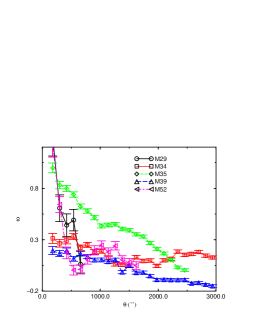
a)

Figure 5: $\omega$ at some regions with visible magnitudes.

Fig. 5 b)

Fig. 5 c)

Hence, the method does indeed detect clustering where there are known to be clusters but not where there is believed to be none. One cluster would be enough if its effect were not too attenuated by foreground and background stars in the chosen range of magnitudes. Moreover, the predictions of the sizes of the clusters is quite acceptable in comparison with the catalogued sizes (see Table LABEL:Tab:clusvis and Figure 6).

Figure 6: $\theta_{\rm max}$, the predicted size of the average cluster according to the simple model used in this paper versus the catalogued size of the cluster in this region (in case of two clusters, the average size of both is plotted).

5.3 Peculiarities of TMGS data in calculating the TPACF

Due to the way in TMGS data is obtained, the following considerations must be taken into account when applying the method and in the examination of the results obtained.

• The method of assigning declinations to the stars in the TMGS will give extra angular correlations in the angles which are multiples of the angular size of the detector (17 arcsec) or multiples of the quarter diameter. Declinations are assigned with discrete values, which are separated by distance multiples of a quarter of the detector size ($\sim 4^{\prime\prime}$). However, the correlation using $\theta$ greater than 4 or 5 arcsec is not significantly affected by this characteristic. The range of $\theta$ to be used in this paper is from $5$ to $250$ arcsec; moreover, $C_{2}$ is averaged over a wide range of $\theta$, much higher than 4 arcsec, so this effect is negligible for this particular case. However, for the correlation of angles smaller than $4$ arcsec this effect could be important.

• The strips do not cover the whole sky; neither do they completely cover 100% of the area of the rectangles that we will use to calculate the angular correlation function. The TMGS (Garzón et al. 1993) was carried out by means of drift scanning with strips of constant declination, and in some cases there are small gaps between adjacent strips which make the sky coverage within the squares in the region of interest incomplete. To correct for this effect, we must multiply $(1+\omega_{\rm t}(\theta))$ by the fraction of area covered in the rectangle with regard the expression (44), assuming that the positions in the rectangle which are not covered is random. The fraction of area covered in the squares that we use is high (greater than $80$ %) so the measure of the error is good enough because it is only affected by a factor of between $\sqrt{0.80}$ and unity.

5.4 Application to TMGS

As an example, two cases will now be applied to the TMGS.

From the TMGS data a rectangular region of the sky was selected centred on $\alpha=16^{\rm h}48^{\rm m}48^{\rm s}$, $\delta=-22^{\circ}26^{\prime}40^{\prime\prime}$ (J2000.0, corresponding to Galactic coordinates $l=-1^{\circ}58^{\prime}15^{\prime\prime}$, $b=14^{\circ}12^{\prime}13^{\prime\prime}$) and sides $0.462^{\circ}$ and $1.626^{\circ}$, respectively, for the directions of $\alpha$ and $\delta$. In this field, the calculation of the TPACF was carried out for stars down to 9.0 mag in $K$. From (42) and (2), we obtain $\omega$ up to $\theta=250^{\prime\prime}$, as presented in Figure 7. An upper limit of $250^{\prime\prime}$ for the value of $\theta_{\rm max}$ is considered. The parameters used in the measure are $\theta_{\rm min}=5^{\prime\prime}$ and $\Delta\theta=5^{\prime\prime}$.

Figure 7: $\omega$ at $l=-1^{\circ}58^{\prime}15^{\prime\prime}$, $b=14^{\circ}12^{\prime}13^{\prime\prime}$.

The result after calculating $\omega$, using (5) is

$$\theta_{\rm max}=62.5^{\prime\prime}\pm 2.5^{\prime\prime}$$

and

$$C_{2}=1.21\pm 0.22.$$

This is an example of a field where some correlation is found ($C_{2}$ is non-zero at the 5.5-$\sigma$ level). Clearly, there is clustering rather than a Poissonian distribution.

As a second example, a rectangular region was chosen centered on $\alpha=18^{\rm h}50^{\rm m}24^{\rm s}$, $\delta=-5^{\circ}14^{\prime}7^{\prime\prime}$ (J2000.0; $l=28^{\circ}10^{\prime}18^{\prime\prime}$, $b=-2^{\circ}8^{\prime}40^{\prime\prime}$) with sides $0.498^{\circ}$ and $0.289^{\circ}$, respectively, for the direction ($\alpha$,$\delta$). Calculation of the angular correlation function was also made for the stars down to 9.0 mag in $K$ for this field.

Using (42) and (2), and with the same parameters as for the previous case, the $\omega$ shown in Fig. 8 is obtained. This gives finally:

$$\theta_{\rm max}=22.5^{\prime\prime}\pm 2.5^{\prime\prime}$$

and

$$C_{2}=3.0\times 10^{-2}\pm 14.6\times 10^{-2}.$$

Figure 8: $\omega$ at $l=28^{\circ}10^{\prime}18^{\prime\prime}$, $b=-2^{\circ}8^{\prime}40^{\prime\prime}$.

In this case the correlation is very weak ($C_{2}$ is $\sim 40$ times smaller than in the previous case), and there is a difference of only $0.2$ $\sigma$ from zero, which, within the errors, implies that there is no correlation or clustering among the stars from this field. Figure 8 shows that $\omega$ is almost zero for every value of $\theta$ within the error bar. The value of $\theta_{\rm max}$ is meaningless in this case, because $\omega$ has such a low value that the error in the search for the first zero of the function is large. When there is little correlation in the field $\theta_{\rm max}$ will be small because the algorithm that eliminates the zeros due to fluctuations does not work well when $\omega$ is much smaller than its error. Also, in this case $\sigma(C_{2})$, the error in $C_{2}$, will be larger than, or of same order as, $C_{2}$. To overcome this problem those data with large $\sigma(C_{2})$ will be separated and only those with $C_{2}>3.5\times\sigma(C_{2})$ will be considered as having confirmed correlations.

5.5 Which clusters can be detected with this procedure?

In the following application, the TPACF will be measured for stars down to $K=9.0$ mag and for a maximum angle of $250^{\prime\prime}$. From Appendix A2, this requires a minimum strip width of $\sim 500^{\prime\prime}$. Larger clusters would be detected with larger angles; however, $250^{\prime\prime}$ is almost the largest angle that can be used if the same analytical criteria are to be applied to all ten TMGS strips that we will use.

A typical open cluster has an average size of $5$ pc (Janes & Phelps 1994), so $500^{\prime\prime}$ will be sufficient to detect it at $\sim 2$ kpc. Therefore, mostly distant clusters will be detected. However, the TMGS is dominated by late K and M giants. Therefore, the majority of the stars detected in the magnitude range to be used are significantly further away than 2 kpc. It is estimated that $\sim 10^{\prime}$ is the maximum size of the clusters which will affect $C_{2}$, although this is difficult to calculate accurately, and the contribution of the largest clusters is not nil but decreases as the cluster increases in size.

The exact calculation of the minimum size is also difficult to analyse. The TMGS survey does not detect the individual sources in globular clusters since the stars are too close to be separated and the whole cluster will appear as an extended source. Similarly, if the open cluster is very small there is excessive overcrowding, or confusion, of sources, a few of them contributing very little to the parameter $C_{2}$. The separation between the stars in a cluster needs to be more than twice the diameter of the detector for its components to be detected, i.e. a minimum of $30^{\prime\prime}$ to $35^{\prime\prime}$.

In conclusion, it is expected to detect distant clusters with angular diameters of between 0.5 and 10 arcmin. Solar neighbourhood clusters, such as M45, will provide only a small contribution to the quantity $C_{2}$, so they will not be detected. Hence the analysis will focus on the large-scale distribution of clusters in the Galaxy.

6 Correlations as a function of Galactic coordinates

When the procedure is used in other regions, the behaviour of $C_{2}$ as a function of $l$ and $b$ can be determined.

Calculations of $\omega(\theta)$ were carried out on several strips with constant declination and various sub-strips (Table LABEL:Tab:zonesdelta). The value of $l$ quoted is that at which the strip intersects the Galactic plane ($b=0^{\circ}$). The range of Galactic latitude is $|b|<15^{\circ}$ for $l<35^{\circ}$ and $|b|<5^{\circ}$ for $l>35^{\circ}$.

Table 3: TMGS regions (with constant declination) used in this paper.

Strip	$\delta$	$l$ at $b=0^{\circ}$	Width of strip
	(deg)	(deg)	(deg)
1	$-29.7$	$-0.9$	$2.51$
2	$-22.4$	$7.5$	$1.63$
3	$-15.6$	$15.4$	$0.78$
4	$-5.2$	$27.1$	$0.29$
5	$-1.6$	$31.2$	$1.50$
6	$3.5$	$36.9$	$0.13$
7	$22.0$	$57.8$	$0.30$
8	$32.5$	$70.1$	$0.35$
9	$39.1$	$167.8$	$0.35$
10	$30.4$	$178.2$	$0.13$

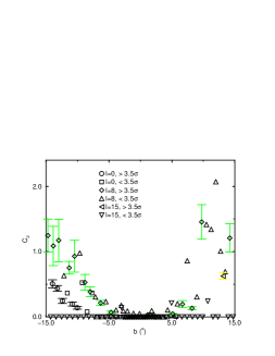
a)

Figure 9: $C_{2}$ at a) $\delta=-30$, $-22$ and $-16$; b) $\delta=-5$, $-1$ and $4$ ; c) $\delta=22$, $33$, $39$ (in the anticenter direction) and $30$ (in the anticenter direction). Points with $C_{2}>3.5\sigma(C_{2})$ are plotted with bar error.

Fig. 9 b)

Fig. 9 c)

The results are plotted in the Figs. 9, those for which $C_{2}>3.5$ $\sigma(C_{2})$ being separated from the others. Not all the strips have the same number of stars, so $\sigma(C_{2})$ is different for different regions. The best strips, with smallest errors, are those which cross the plane at $l=-1^{\circ}$, $l=8^{\circ}$ and $l=31^{\circ}$, i.e. strips 1, 2 and 5 respectively. The main features observed are:

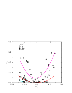
Figure 10: Fit of $C_{2}$ of strips 1, 2 and 5 (those that are greater than $3.5\ \sigma(C_{2})$) to respective parabollic functions: $2.2\times 10^{-3}b^{2}$, $6.4\times 10^{-3}b^{2}$ and $20\times 10^{-3}b^{2}+0.036b+1.0$ (solid lines).

1. There is general a $C_{2}$ dependence on Galactic latitude in the disc for $l<90^{\circ}$ (i.e. strips 1-8 ) with some exceptions pointed out in (iv). This relationship is especially remarkable in strips 1, 2 and 5. The function $C_{2}(b)$ is approximately parabolic. Figure 10 shows the following fits to the best data (those with $C_{2}>3.5\ \sigma(C_{2})$) of these strips:

   $$C_{2}=2.2\times 10^{-3}b^{2}\ \ {\rm for}\ l=0^{\circ},$$ (46)

   $$C_{2}=6.4\times 10^{-3}b^{2}\ \ {\rm for}\ l=8^{\circ}$$ (47)

   and

   $$C_{2}=20\times 10^{-3}b^{2}+0.036b+1.00\ \ {\rm for}\ l=31^{\circ}.$$ (48)

2. Outside the bulge, there is a general increase in $C_{2}$ with $l$, as seen in equations (46), (47) and (48). When the data with $C_{2}>3.5$ $\sigma(C_{2})$ are averaged between $b=-3^{\circ}$ and $b=3^{\circ}$, and also for $3^{\circ}<|b|<5^{\circ}$, there is a dependence on $l$ as shown in Table LABEL:Tab:depend_l.

3. In the inner bulge region, with $l<15^{\circ}$ and $b<5^{\circ}$, the correlations are almost zero (Fig. 9 a)). When the relative correlation differences at $l\sim 30^{\circ}$ and the inner bulge are compared with those predicted by the simple model (Figs. 4, 3) a correlation deficit can be seen for the bulge.

4. Three regions where there is an excess of correlation with respect to both the $l$ and $b$ dependence occur at at $l=31^{\circ}$, $l=37^{\circ}$ (Fig. 9b) and $l=70^{\circ}$ (Fig. 9c), i.e. strips 5, 6 and 8.

5. The anticentre region gives a correlation similar to that of the intermediate Galactic longitude ($50^{\circ}<l<100^{\circ}$) region in the plane, or even lower (see Table LABEL:Tab:depend_l). The value of $C_{2}$ does not increase with $l$, or it does so very smoothly outside the intermediate $l$ region. The simple model prediction is not very accurate but, comparing with the results in Figs. 3 and 4, it can be seen that $C_{2}$ is larger at $l\sim 150^{\circ}$ than at $l\sim 40^{\circ}$. This significant departure cannot be explained without including an extra component in the model.

Table 4: The $C_{2}$ dependence on $l$.

Strip	$l$ at $b=0^{\circ}$	$\overline{C_{2}}$ in $|b|<3^{\circ}$	$\overline{C_{2}}$ in $3^{\circ}<|b|<5^{\circ}$
	(deg)
1	$-1$	–	–
2	$8$	$3.5\times 10^{-2}$	$6.9\times 10^{-2}$
3	$15$	–	–
4	$27$	–	–
5	$31$	$0.38$	$1.29$
6	$37$	$0.90$	$3.01$
7	$58$	$0.74$	$0.97$
8	$70$	$1.26$	$1.08$
9	$168$	$0.78$	$0.71$
10	$178$	$0.67$	–

6.1 Causes of the dependence on Galactic coordinates

1. The $b$-dependence: This is predicted by the simple model created above. As seen in Fig. 4, $\omega$ should increase with $|b|$ because $\langle n_{\rm cl}\rangle\left((\rho_{\rm cl}-\rho_{\rm nc})/\langle\rho\rangle\right)^{2}$ in expression (29) increases with $|b|$.

2. The $l$-dependence: Again, the $l$-dependence can be explained by the model.

3. The bulge: When $C_{2}$ values for bulge regions are compared with those for other regions where there is only a disc component, the observational data give a lower relative correlation than is prediced by the model (Fig. 3), i.e. there is less correlation in the bulge than expected. This is consistent with the bulge being older than the disc (see Section 4.1). The bulge is known to have a different population of stars from the disc (Frogel 1988; López Corredoira et al. 1997), and these are expected to be an older population (Rich 1993), so the lack of correlation would be expected. Moreover, as pointed out earlier, the central region will have patchy extinction which will tend to increase the correlation. Hence, the $C_{2}$ values generated by clusters should be even lower than the observed value indicating even fewer young clusters in this region.

4. Excess correlation in some zones in the plane: Feinstein (1995) points out that very young clusters are tracers of the spiral arms. As has been noted young clusters provide a significant contribution to $C_{2}$. However, spiral arms are not included in the simple model, which contains only the disc and bulge; hence where an arm is crossed it is to be expected that the correlation will be higher than predicted. Whereas the distribution of old clusters varies smoothly with Galactic position, the young clusters have a far more irregular distribution.

   Of the four areas which cross the plane between $l=31^{\circ}$ and $l=70^{\circ}$ three show a significant correlation excess. The $l=31^{\circ}$ region is almost tangential to the Scutum arm and also runs through the Sagittarius arm. The $l=37^{\circ}$ region will also cut the Sagittarius arm. The excess correlation at $l=70^{\circ}$ can be attribute to the star formation region in the Perseus arm. The far-infrared source G69C in this region has been attributed to star formation regions by Kutner (1987). Strip 7 ($l=58^{\circ}$) is an exception which could possibly be due to this line of sight missing a significant star formation region as it crosses the arm.

   Using the simple model described previously with one shell of clusters (Section 3.1) but only allowing clusters in the arms, the degree of clustering in the arm can be estimated. With the use of (34) a relationship between various cluster parameters can be obtained (for example, at $l\approx 70^{\circ}$, $b\approx 0^{\circ}$, $C_{2}$ is $1.88\pm 0.34$). It is assumed that the greater part of the contribution to $C_{2}$ is due to the arm clusters, and that, as estimated by Cohen et al. (1997, in preparation) $\sim 30$% of the stars observed in that region are from the arm (with $\Delta r\approx 1$ kpc in the line of sight), whereas the rest belongs to the disc. As $\theta_{\rm max}$ is $46.5^{\prime\prime}$ in this region, the equivalent cluster diameter, from (33), is $2.0$ pc (when the distance is $r=8.8$ kpc; Georgelin & Georgelin 1976). This is smaller than the average value of $5$ pc given by Janes & Phelps (1994), although this could possibly be due to the fact that only the core of the cluster is seen by the TMGS (the typical size of the core of a cluster is 1 or 2 pc; Leonard 1988), in which there are bright and more massive stars; alternatively, a possible difference from the solar neighbourhood could also be the explanation. Nevertheless, this is only a rough estimate and no further conclusions should be drawn from this number. The order of magnitude should, however, be correct.

   With these data it possible to estimate the density of stars within the clusters. Using (34) gives

   $$\langle n_{\rm cl}\rangle\approx 3\times 10^{4}\left(\frac{\rho_{\rm cl}-\rho_{\rm nc}}{\langle\rho\rangle}\right)^{-2},$$ (49)

   or, making use of (23) with $\frac{4}{3}\pi R_{\rm cl}^{3}\langle n_{\rm cl}\rangle\ll 1$ and $\rho_{\rm nc}\ll\rho_{\rm cl}$,

   $$\langle n_{\rm cl}\rangle\approx 3\times 10^{4}\left[\frac{\frac{4}{3}\pi R_{\rm cl}^{3}\langle n_{\rm cl}\rangle\rho_{\rm cl}+\rho_{\rm nc}}{\rho_{\rm cl}}\right]^{2}.$$ (50)

   When $\langle n_{\rm cl}\rangle$ is determined with last equation, the following condition is then derived for solving the second-degree equation with real numbers:

   $$\rho_{\rm nc}<2\times 10^{-6}\rho_{\rm cl}$$ (51)

   and

   $$5\times 10^{-7}\ {\rm pc}^{-3}<{\rm\langle}n_{\rm cl}{\rm\rangle}<2\times 10^{-6}\ {\rm pc}^{-3},$$ (52)

   which is equivalent to saying that most of the stars within the arm in this line of sight are forming clusters. Indeed, with such a low $\rho_{\rm nc}$ (because of (51)), by (23) and (52) gives

   $$10^{5}\langle\rho\rangle\ \ <\ \ \rho_{\rm cl}\ \ <\ \ 5\times 10^{5}\langle\rho\rangle,$$ (53)

   which, with $\langle\rho\rangle\sim 1.4\times 10^{-3}\ {\rm pc}^{-3}$ (From the Galaxy model used in Wainscoat et al. 1992), gives

   $$140\ {\rm pc}^{-3}<\rho_{\rm cl}<700\ {\rm pc}^{-3},$$ (54)

   i.e. between $500$ and $3000$ stars per cluster, a quite reasonable number (Friel 1995 talks about a typical mass of young clusters of few thousand solar masses).

   The same case is repeated at $l=37^{\circ}$ and at $l=31^{\circ}$. When the line of sight cuts an arm, the correlation is greatly increased. If the arm contribution to the number of stars is low, the correlation will be diluted, although its contribution may be not totally negligible. It also depends on the density of the other components for that direction; the disc, for example, dilutes the correlation.

   Hammersley et al. (1994) and Garzón et al. (1997) suggest that there should be an excess of bright stars in the region at $l=27^{\circ}$, $b=0^{\circ}$ which might be due to the interaction of a bar with the disc, giving rise to a star formation region. Concerning the deficit of correlation measured for this star formation region, it could be concluded that, if the star formation were sufficiently large–much greater, say, than the size of the rectangle used from sampling–then this would explain the non-detection of clustering in this region.

5. Deviation from a simple model of $l$ dependence in the anticentre: Towards the anticentre ($210^{\circ}>l>150^{\circ}$) the correlation is significantly less than that predicted by the simple model. This implies that the number of clusters is small and, in particular, that very young clusters are rare in this direction. This is in agreement with the results from visible observations of clusters (Payne-Gaposchkin 1979). Janes & Phelps (1994) argue that there is a lack of old clusters in the inner disc, since they would be destroyed by molecular clouds (see Section 4.1), but that there will a relatively large number of young clusters. However, the ISM density falls off with distance from the Galactic centre, so in the outer disc there will be significantly less star formation and hence far fewer young clusters. The existence of a gradient in open cluster age has been commented on by Lyngå (1980) and Van den Bergh & McClure (1980), and an explanation was attempted by Wielen (1985). As has been noted previously, young clusters contribute significantly to $C_{2}$, so the lack of young clusters in the anticentre region would lead to a reduction in the amount of correlation.

   Within a few degrees of the plane the arms have a significant influence on the amount of correlation for the longitude range $30^{\circ}<l<90^{\circ}$. One possible reason for the apparent deficit in $C_{2}$ towards the anticentre could be the excess due to the arms in the comparison regions. In order to discount this possibility, a comparison of the in-plane anticentre region can be made with an off-plane region at $l=31^{\circ}$. The model predicts that the ratio $C_{2}(l$$=$$31^{\circ},$$5^{\circ}$$<$$|$$b$$|$$<$$15^{\circ})$$/$$C_{2}(l$$=$$168^{\circ},$$|$$b$$|$$<$$5^{\circ})$ should be less than unity, however, the measurements give a value of 4 or 5. This gives further support to the hypothesis that there are fewer young clusters than expected towards the anticentre.

   A further possible reason for the lack of correlation in the anticentre is that there could be a significant decrease in the total numbers of clusters in the anticentre rather then an increase of age with Galactocentric distance. However, observations in the solar neighbourhood (Lyngå 1980; Van den Bergh & McClure 1980; Janes & Phelps 1994) support the hypothesis of increasing age of the clusters with Galactocentric distance.

   Also, clusters in the anticentre have a greater angular size because they are nearer but this is taken into account in the model and should not cause the deficit of correlation.

   When the analysis presented here is applied to other large-area infrared observations it may contribute to our understandanding of this dependence on cluster age on Galactocentric distance. The TMGS data clearly shows the presence of young clusters in the inner Galaxy and consequently a decrease in $C_{2}$ in the anticentre direction. However, An accurate quantification is not possible because of arm contamination in most parts of the regions, for which complete information is unavailable.

7 Conclusions

A technique is developed for searching for clustering in stellar surveys using correlation functions. The mathematical tools are useful for any field of stars and can be applied to any survey, especially those at carried out at infrared wavelengths, which permit a study of the distribution of stars throughout almost the entire Galaxy. The DENIS (Epchtein 1997) or 2MASS (Skrutskie et al. 1997) surveys will be ideal for this technique as the increased numbers of stars will reduce the errors. It is even possible, with a large number of stars in the survey, to apply the technique for different ranges of apparent magnitude. Studying the clustering of stars at different apparent magnitudes is equivalent to do studying in three dimensions ($l$, $b$ and the average distance $\overline{r}$ which is associated with the treated range of magnitudes).

A simple model has been developed. This model could be improved by introducing a density dependence as a function of the distance from the centre of the cluster, perhaps a power-law dependence.

In this paper the method has been applied to the TMGS. Is has been shown that a simple model in which old open clusters trace the whole Galaxy with a density of clusters proportional to the density of stars agrees quite well with the data. An exception to the general agreement are specific regions in the plane where the higher-than-expected clustering can be attributed to star formation in the spiral arms. A second departure from the simple model is the reduced $C_{2}$ in the outer disc and in the bulge due to a lack of young clusters.

In one of the regions with an excess, at $l=70^{\circ}$ in the plane, the approximate limits for the cluster density and the density of stars inside the cluster are derived. These are, respectively, $5\times 10^{-7}\ {\rm pc}^{-3}<{\rm\langle}n_{\rm cl}{\rm\rangle}<2\times 10^{-6}\ {\rm pc}^{-3}$ and $140\ {\rm pc}^{-3}<\rho_{\rm cl}<700\ {\rm pc}^{-3}$. There is, however, a lower-than-expected correlation at $l=27^{\circ}$, $b=0^{\circ}$. There is believed to be a huge star formation region in this direction and the lack of correlation could be due to the star formation region being far larger than the sample area.

As has been pointed out by Friel (1995), the oldest open clusters may be viewed from two perspectives with regard the formation of the Galaxy: a halo collapse or a continuous accretion and infall of material from the halo on to the Galactic disc. Either perspective is possible. The first should justify which were the original star formation regions that were the origin of the present old clusters in the outer disc and how they travelled there from their place of origin. The second perspective needs to test the infall of matter from the halo as well as the existence of star systems in the halo. Further improvements on these cluster searches and better numbers will give us a hint concerning these questions on the origin of the Galaxy. A better determination of $C_{2}$ in the bulge region will tell us about the age of bulge clusters if these exist. In this article we have observed a relative absence of correlation in the bulge that is somewhat less than the prediction of our simple model, but at best the prediction could say, as in the case of the anticentre, whether the correlation is greater or less than the improved model and enable us to reach further conclusions.

Acknowledgments

We thank the anonymous referees for helpful comments that have substantially improved the content and presentation of this paper.

Appendix A Calculations for two intersecting spheres

The centres of two spheres are separated by a distance $x$, and $S_{\rm ss}(x;y,R_{\rm cl})$ is the area of the shell of the first sphere (the one with radius $y$) contained in the second sphere (Betancort-Rijo 1995), with radius $R_{\rm cl}$ (see Fig. 1). There are various cases:

1. $R_{\rm cl}>y$:

   1. $x<(R_{\rm cl}-y)$: the first sphere is contained wholly within the second sphere, so that the area of the shell that is inside the second sphere is the area of the whole shell, and

      $$S_{\rm ss}(x;y,R_{\rm cl})=4\pi y^{2}.$$ (55)

   2. $(R_{\rm cl}-y)<x<(R_{\rm cl}+y)$: this is the area of the shell for $\theta$ up to $\theta_{0}$, according to Fig. 1; simple trigonometry gives the value of $\theta_{0}$ (as a function of $x$, $y$ and $R_{\rm cl}$) as

      $$R_{\rm cl}^{2}=x^{2}+y^{2}-2xy\cos\theta_{0}$$ (56)

      $$\cos\theta_{0}=\frac{x^{2}+y^{2}-R_{\rm cl}^{2}}{-2xy},$$ (57)

      and the area of the shell up to $\theta_{0}$ is

      $$S_{\rm ss}(x;y,R_{\rm cl})=2\pi y^{2}\int_{0}^{\theta_{0}}d\theta\ \sin\theta$$

      $$=2\pi y^{2}(1-\cos\theta_{0}),$$ (58)

      so that, changing $\theta_{0}$ by the value given in (57), we get:

      $$S_{\rm ss}(x;y,R_{\rm cl})=\frac{\pi y}{x}(R_{\rm cl}^{2}-(x-y)^{2}).$$ (59)

2. $R_{\rm cl}<y$:

   1. $x<(y-R_{\rm cl})$: here there is no contact between the shell and the second sphere, so

      $$S_{\rm ss}(x;y,R_{\rm cl})=0.$$ (60)

   2. $(y-R_{\rm cl})<x<(y+R_{\rm cl})$: again, the calculation proceeds as for (59):

      $$S_{\rm ss}(x;y,R_{\rm cl})=\frac{\pi y}{x}(R_{\rm cl}^{2}-(x-y)^{2}).$$ (61)

Quantities that we are interested for calculating are $\int_{0}^{R_{\rm cl}}dx\ x^{2}S_{\rm ss}(x;y,R_{\rm cl})$ and $\int_{R_{\rm cl}}^{R_{\rm cl}+y}dx$ $\times x^{2}S_{\rm ss}(x;y,R_{\rm cl})$. Again, we distinguish several cases:

1. $y<R_{\rm cl}$: following (55) and (59),

   $$\int_{0}^{R_{\rm cl}}dx\ x^{2}S_{\rm ss}(x;y,R_{\rm cl})=\int_{0}^{R_{\rm cl}-y}dx\ x^{2}4\pi y^{2}$$

   $$+\int_{R_{\rm cl}-y}^{R_{\rm cl}}dx\ x^{2}\frac{\pi y}{x}(R_{\rm cl}^{2}-(x-y)^{2})$$

   $$=\frac{4}{3}\pi R_{\rm cl}^{3}y^{2}\left(1-\frac{3}{4}\frac{y}{R_{\rm cl}}+\frac{1}{16}\left(\frac{y}{R_{\rm cl}}\right)^{3}\right)$$ (62)

   and

   $$\int_{R_{\rm cl}}^{R_{\rm cl}+y}dx\ x^{2}S_{\rm ss}(x;y,R_{\rm cl})$$

   $$=\int_{R_{\rm cl}}^{R_{\rm cl}+y}dx\ x^{2}\frac{\pi y}{x}(R_{\rm cl}^{2}-(x-y)^{2})$$

   $$=\frac{4}{3}\pi R_{\rm cl}^{3}y^{2}\left(\frac{3}{4}\frac{y}{R_{\rm cl}}-\frac{1}{16}\left(\frac{y}{R_{\rm cl}}\right)^{3}\right).$$ (63)

2. $R_{\rm cl}<y<2R_{\rm cl}$: following (60) and (61),

   $$\int_{0}^{R_{\rm cl}}dx\ x^{2}S_{\rm ss}(x;y,R_{\rm cl})$$

   $$=\int_{y-R_{\rm cl}}^{R_{\rm cl}}dx\ x^{2}\frac{\pi y}{x}(R_{\rm cl}^{2}-(x-y)^{2})$$

   $$=\frac{4}{3}\pi R_{\rm cl}^{3}y^{2}\left(1-\frac{3}{4}\frac{y}{R_{\rm cl}}+\frac{1}{16}\left(\frac{y}{R_{\rm cl}}\right)^{3}\right)$$ (64)

   and

   $$\int_{R_{\rm cl}}^{R_{\rm cl}+y}dx\ x^{2}S_{\rm ss}(x;y,R_{\rm cl})$$

   $$=\int_{R_{\rm cl}}^{R_{\rm cl}+y}dx\ x^{2}\frac{\pi y}{x}(R_{\rm cl}^{2}-(x-y)^{2})$$

   $$=\frac{4}{3}\pi R_{\rm cl}^{3}y^{2}\left(\frac{3}{4}\frac{y}{R_{\rm cl}}-\frac{1}{16}\left(\frac{y}{R_{\rm cl}}\right)^{3}\right).$$ (65)

3. $y>2R_{\rm cl}$: again, with (60) and (61),

   $$\int_{0}^{R_{\rm cl}}dx\ x^{2}S_{ss}(x;y,R_{\rm cl})=0$$ (66)

   and

   $$\int_{R_{\rm cl}}^{R_{\rm cl}+y}dx\ x^{2}S_{\rm ss}(x;y,R_{\rm cl})$$

   $$=\int_{y-R_{\rm cl}}^{R_{\rm cl}+y}dx\ x^{2}\frac{\pi y}{x}(R_{\rm cl}^{2}-(x-y)^{2})=\frac{4}{3}\pi R_{\rm cl}^{3}y^{2}.$$ (67)

Appendix B Edge effects in the measurement of the TPACF in rectangular fields

We have a rectangular surface with size $a\times b$ ($x$ from $0$ to $a$ and $y$ from $0$ to $b$). A ring of negligible thickness and of radius $\theta$ whose centre is located at $(x,y)$ contains part of the surface inside the rectangle, $f(x,y)$, and the rest of it is outside the rectangle. Due to the loss of a part of the ring surface outside the rectangle we measure only a fraction $F_{\rm BE}$ of the star counts separated by an angular distance $\theta$. Assuming that the distribution of the stars in the rectangle is homogeneous, we have

$$F_{\rm BE}=\frac{1}{a\ b}\int_{0}^{a}dx\int_{0}^{b}dyf(x,y).$$ (68)

The value of $f(x,y)$ depends on the case. With the condition $2\theta<a$, $2\theta<b$ (which is to be satisfied in the case considered here), the only posibilities are:

1. when $\theta<x<(a-\theta)$ and $\theta<y<(b-\theta)$: the whole ring is inside the rectangle, so

   $$f(x,y)=1.$$ (69)

2. when $\theta<x<(a-\theta)$ and $y<\theta$: the portion of ring contained inside the rectangle is from the angle $-\sin^{-1}(y/\theta)$ to $\pi+\sin^{-1}(y/\theta)$ (the value of $\sin^{-1}(\cdots)$ between 0 and $\pi/2$). Then,

   $$f(x,y)=\frac{\pi+2\sin^{-1}(y/\theta)}{2\pi}.$$ (70)

3. when $x<\theta$ and $\theta<y<(b-\theta)$: similarly to the previous case:

   $$f(x,y)=\frac{\pi+2\sin^{-1}(x/\theta)}{2\pi}.$$ (71)

4. when $x<\theta$, $y<\theta$ and $(x^{2}+y^{2})<\theta^{2}$: the portion of ring inside the rectangle is from the angle $-\sin^{-1}(y/\theta)$ to $\pi/2+\sin^{-1}(x/\theta)$, so

   $$f(x,y)=\frac{\pi/2+\sin^{-1}(x/\theta)+\sin^{-1}(y/\theta)}{2\pi}.$$ (72)

5. when $x<\theta$, $y<\theta$ and $(x^{2}+y^{2})>\theta^{2}$: this case is similar to the previous one, but we must add another portion of ring which is between $-(\pi/2+\sin^{-1}(x/\theta))$ and $\pi+\sin^{-1}(y/\theta)$, so

   $$f(x,y)=\frac{2\sin^{-1}(x/\theta)+2\sin^{-1}(y/\theta)}{2\pi}.$$ (73)

Other possible situations are avoided by the symmetry properties of the integral used in the evaluation of $F_{\rm BE}$, which is reduced to the following calculation:

$$F_{\rm BE}(\theta)=\frac{1}{a\ b}[(a-2\theta)(b-2\theta)]$$

$$+\frac{2}{a\ b}\left[\int_{\theta}^{a-\theta}dx\int_{0}^{\theta}dy\frac{\pi+2\sin^{-1}(y/r)}{2\pi}\right]$$

$$+\frac{2}{a\ b}\left[\int_{\theta}^{b-\theta}dy\int_{0}^{\theta}dx\frac{\pi+2\sin^{-1}(x/r)}{2\pi}\right]$$

$$+\frac{4}{a\ b}\left[\int_{0}^{\theta}dx\int_{0}^{\theta}dy\frac{\pi/2+\sin^{-1}(x/r)+\sin^{-1}(y/r)}{2\pi}\right]$$

$$+\frac{4}{a\ b}\left[\int_{0}^{\theta}dx\int_{\sqrt{\theta^{2}-x^{2}}}^{\theta}dy\frac{-\pi/2+\sin^{-1}(x/r)+\sin^{-1}(y/r)}{2\pi}\right]$$

$$=1-\frac{2}{\pi}\left(\frac{1}{a}+\frac{1}{b}\right)\theta+\left(\frac{9}{\pi}+\frac{\pi}{2}-4\right)\frac{1}{a\ b}\theta^{2}.$$ (74)

References

- [\citeauthoryear] Allen C. W., 1973, Astrophysical Quantities, 3rd ed. Athlone Press, London
- [\citeauthoryearBahcall1986] Bahcall J. N., 1986, ARA&A, 24, 577
- [\citeauthoryear] Balázs L. G., 1995, Mem S. A. It., 66, 689
- [\citeauthoryear] Betancort-Rijo J., 1991, A&A, 245, 347
- [\citeauthoryear] Betancort-Rijo J., 1995, private communication
- [\citeauthoryear] Boggess N. W., Mather J. C., Weiss R., et al., 1992, ApJ, 397, 420
- [\citeauthoryear] Borgani S., 1995, Physics Rep., 251, 1
- [\citeauthoryear] Carraro G., Chiosi C., 1994, A&A, 287, 761
- [\citeauthoryear] Chandrasekhar S., 1942, Principles of stellar dynamics. Chicago University Press, Chicago, ch. 5
- [\citeauthoryear] Chandrasekhar S., 1943a, ApJ, 97, 255
- [\citeauthoryear] Chandrasekhar S., 1943b, ApJ, 97, 263
- [\citeauthoryear] Chandrasekhar S., 1943c, ApJ, 98, 54
- [\citeauthoryear] Dwek E., Arendt R. G., Hauser M. G., et al., 1995, ApJ, 445, 716
- [\citeauthoryear] Epchtein, N., 1997, in Garzón F., Epchtein N., Omont A., Burton B., Persi P., eds., The Impact of Large Scale Near-IR Sky Survey. Kluwer, Dordrecht, p. 15
- [\citeauthoryear] Fall S. M., Tremaine S., 1977, ApJ, 216, 682
- [\citeauthoryear] Feinstein A., 1995, in Alfaro A. J., Delgado A. F., eds., The formation of the Milky Way. Cambridge University Press, Cambridge, p. 56
- [\citeauthoryear] Friel E. D., 1995, ARA&A, 33, 381
- [\citeauthoryear] Frogel J. A., 1988, ARA&A, 26, 51
- [\citeauthoryear] Garzón F., Hammersley P. L., Mahoney T., et al., 1993, MNRAS, 264, 773
- [\citeauthoryear] Garzón F., López-Corredoira M., Hammersley P. L., et al., 1997, ApJ, 491, L31
- [\citeauthoryear] Georgelin Y. M., Georgelin Y. P., 1976, A&A, 49, 57
- [\citeauthoryear] Hammersley P. L., Garzón F., Mahoney T., Calbet X., 1994, MNRAS, 269, 753
- [\citeauthoryear] Janes K. A., Phelps R. L., 1994, AJ, 108, 1773
- [\citeauthoryear] Kutner M. L., 1987, in Peimbert M., Jugaku J., eds., Proc. IAU Symp. 115, Star forming regions. Reidel, Dordrecht, p. 483
- [\citeauthoryear] Leonard P. J. T., 1988, AJ, 95, 108
- [\citeauthoryear] Limber D. N., 1953, ApJ, 117, 134
- [\citeauthoryear] López-Corredoira M., Garzón F., Hammersley P. L., Mahoney T. J., Calbet X., 1997, MNRAS, 292, L15
- [\citeauthoryear] Lyngå G., 1980, in Hesser J. E., ed., Proc. IAU Symp. 85, Star Clusters. Reidel, Dordrecht, p. 13
- [\citeauthoryear] Lyngå G., 1987a, Catalog of Open Clusters, Centre de Donnes Stellaires, Strasbourg
- [\citeauthoryear] Lyngå G., 1987b, in Palou J., ed., Proceedings on 10th European Regional Astronomy Meeting of the IAU, Evolution of Galaxies, Astronomical Institute of the Czechoslovakian Academy of Science, Prague, p. 121
- [\citeauthoryear] Maihara T., Oda N., Sugiyama T., Okuda H., 1978, PASJ, 30, 1
- [\citeauthoryear] Pásztor L., Tóth L. V., 1995, in Shaw R. A., Payne H. E., Hayes J. J. E., eds., ASP Conf. Ser., vol. 77, Astronomical Data Analysis Software and Systems IV. Astronomical Society of the Pacific, San Francisco, p. 319
- [\citeauthoryear] Pásztor L., Tóth L. V., Balázs G., 1993, A&A, 268, 108
- [\citeauthoryear] Payne-Gaposchkin C., 1979, Stars and clusters. Harvard University Press, Harvard, ch. 11
- [\citeauthoryear] Peebles P. J. E., 1980, Large-Scale Structure of the Universe. Princeton University Press, Princeton, ch. 3
- [\citeauthoryear] Pfenninger D., Combes F., 1994, A&A, 285, 94
- [\citeauthoryear] Rhoads J. E., 1995, Bull. American Astron. Soc., 27, 1415
- [\citeauthoryear] Rich R. M., 1993, in S. R. Majewski, ed., ASP Conference Series, Vol. 49, Galactic Evolution: The Milky Way Perspective. Astronomical Society of the Pacific, San Francisco, p. 65
- [\citeauthoryear] Rivolo A. R., 1986, ApJ, 301, 70
- [\citeauthoryear] Skrutskie M. F., Schneider S. E., Stiening R., et al., 1997, in Garzón F., Epchtein N., Omont A., Burton B., Persi P., eds., The impact of Large Scale Near-IR Sky Surveys. Kluwer, Dordrecht, p. 25
- [\citeauthoryear] Spitzer L., 1958, ApJ, 127, 544
- [\citeauthoryear] Terlevich E., 1987, MNRAS, 224, 193
- [\citeauthoryear] Van den Berg S., McClure R. D., 1980, A&A, 88, 360
- [\citeauthoryear] Wainscoat R. J., Cohen M., Volk K., Walker H. J., Schwartz D. E., 1992, ApJS, 83, 111
- [\citeauthoryear] Wiedenmann G., Atmanspacher H., 1990, A&A, 229, 283
- [\citeauthoryear] Wielen R., 1985, in Goodman J., Hut P., eds., Proc. IAU Symp. 113, Dynamics of Star clusters. Reidel, Dordrecht, p. 446
- [\citeauthoryear] Wielen R., Fuchs B., 1988, in Blitz L., Lockman F. J., eds., Outer Galaxy. Springer, Berlin, p. 100
- [\citeauthoryear] Wynn-Williams C. G., 1977, in de Jong T., Maeder A, eds., Proc. IAU Symp. 75, Infrared observations of star formation regions. Reidel, Dordrecht, p. 105