HST images of a galaxy group at $z=2.81$, and the sizes of damped Ly$\alpha$ galaxies

Abstract

We present HST WFPC2 observations in three bands (F450W=B, F467M and F814W=I) of a group of three galaxies at $z=2.8$ discovered in a ground-based narrow-band search for Ly$\alpha\,$emission near the $z=2.8$ quasar PKS $0528-250\,$. One of the galaxies is a damped Ly$\alpha\,$(DLA) absorber and these observations bear on the relation between the DLA clouds and the Lyman-break galaxies and the stage in the evolution of galaxies they represent. We describe a procedure for combining the undersampled WFPC2 images pointed on a sub-pixel grid, which largely recovers the full sampling of the WFPC2 point spread function (psf). These three galaxies have similar properties to the Lyman-break galaxies except that they have strong Ly$\alpha\,$emission. The three galaxies are detected in all three bands, with average $m_{B}\sim 26$, $m_{I}\sim 25$. Two of the galaxies are compact with intrinsic (i.e. after correcting for the effect of the psf) half-light radii of $\sim 0.1$ arcsec ($0.4h^{-1}$ kpc, $q_{\circ}=0.5$). The third galaxy comprises two similarly compact components separated by 0.3 arcsec. The HST images and a new ground-based Ly$\alpha\,$image of the field provide evidence that the three galaxies are more extended in the light of Ly$\alpha\,$than in the continuum. Combined with the evidence from the Ly$\alpha\,$line widths, previously measured, this suggests that we are measuring the size of the surface of last scattering of the escaping resonantly-scattered Ly$\alpha\,$photons. The measured impact parameters for this DLA galaxy (1.17 arcsec), for a second confirmed system, and for several candidates, provide a preliminary estimate of the cross-section-weighted mean radius of the DLA gas clouds at $z\sim 3$ of $<13h^{-1}$ kpc, for $q_{\circ}=0.5$. The true value is likely substantially smaller than this limit as DLA clouds at small impact parameter are harder to detect. Given the observed sky covering factor of the absorbers this implies that for $q_{\circ}=0.5$ the space density of DLA clouds at these redshifts is more than five times the space density of spiral galaxies locally, with the actual ratio probably considerably greater. For $q_{\circ}=0.0$ there is no evidence as yet that DLA clouds are more common than spiral galaxies locally. We summarise evidence that filamentary structures occur in the distribution of galaxies at high redshift.

1 Introduction

By studying typical galaxies at high redshift, here $z>2$, we can record the origins of normal galaxies such as our own Milky Way. Schmidt [1965] was the first to observe a high$-$redshift galaxy when he obtained a spectrum of 3C9, a radio$-$loud quasar of redshift $z=2.01$. Normal star$-$forming high$-$redshift galaxies are about 1000 times fainter, and remained undiscovered until the present decade. A small number of candidates (some of which may be active galaxies) have been identified with 4$-$metre telescopes, through the detection of Ly$\alpha$ emission (e.g. Steidel, Sargent, and Dickinson 1991, Lowenthal et al. 1991, Møller and Warren 1993, Pascarelle et al. 1996, Francis et al. 1995). Another approach has been to employ deep broad$-$band imaging to identify candidates by the expected Lyman$-$limit discontinuity in their spectra (Steidel and Hamilton 1992). The brightest Lyman$-$break galaxies have $m_{R}\sim 24$ and spectroscopic confirmation has only become feasible with the completion of the Keck 10$-$metre telescope. The report by Steidel et al. (1996) on the results of spectroscopic observations of Lyman$-$break candidates really marked the beginning of the statistical study of high-redshift galaxies. They were able to confirm redshifts for 15 star$-$forming galaxies in the range $3.0<z<3.5$. They discovered that Lyman$-$break galaxies generally show weak Ly$\alpha$ emission, but that the rest$-$frame ultra$-$violet spectra may be recognised by the presence of absorption lines characteristic of the spectra of nearby star$-$forming galaxies. Madau et al. (1996) applied the same methodology to the Hubble Deep Field data to extend the results to fainter magnitudes, and their analysis currently provides the best lower limits to the integrated star formation rate in galaxies at $z>2$.

Complementary to the searches for starlight from high$-$redshift galaxies have been the analyses of absorption lines in the spectra of high$-$redshift quasars. These studies have provided measurements of the mass density of neutral hydrogen in the universe (e.g. Wolfe et al. 1986, Lanzetta et al. 1991), and the metallicity of the gas (e.g. Pettini et al 1994), and how these quantities have changed with redshift. The analysis of Pei and Fall (1995) of the absorption–line data reconstructs the global history of star formation, gas consumption, and chemical enrichment, accounting in a self–consistent way for the effects of the progressive extinction of the background quasars due to dust as star formation proceeds. The advantage of the absorption–line approach to the history of star formation is that it is global in nature as all the neutral gas at any redshift is directly observed. With the deep imaging studies it is necessary to extrapolate below the survey flux limit to measure the total star formation rate.

The weakness of the global approach however is that it tells us nothing about the sizes and morphologies of the galaxies in which the star formation occurs. Deep imaging of DLA absorbers provides the missing information. In other words if we imaged the absorbers we could combine the data of faint galaxy surveys (luminosities, sizes, shapes) with the information on the gas obtained from the spectroscopic studies (column densities, chemistry), allowing a more detailed comparison with theories of galaxy formation.

Unlike for MgII absorbers (e.g. Bergeron and Boissé 1991, Steidel, Dickinson, and Persson 1994a) little progress has been made in such a programme of imaging of DLA systems. There are only two published unambiguous detections, discussed below, as well as a small number of candidate counterparts of DLA absorbers (at both low redshift $-$ Steidel et al. 1994b, Le Brun et al. 1997 $-$ and high-redshift $-$ Aragón-Salamanca et al. 1996). In this paper we report on the results of 30 orbits of imaging observations with the Hubble Space Telescope (HST) of a group of three galaxies at $z=2.81$, named S1, S2, S3, one of which (S1) is a damped Ly$\alpha\,$absorber. The three galaxies lie in the field of the quasar PKS $0528-250\,$, and were detected in the light of Ly$\alpha\,$emission by Møller and Warren (1993, hereafter Paper I). A detailed discussion of their nature was presented by Warren and Møller (1996, hereafter Paper II ). The HST images provide measures of their sizes, magnitudes, and colours. The other high$-$redshift damped system that has been successfully imaged is the absorber at $z=3.150$, towards the quasar $2231+131$, observed by Djorgovski et al. [1996]. In this paper we intercompare the measured properties of these two absorbers, the two companion galaxies S2 and S3, and the population of Lyman$-$break galaxies, to draw conclusions about the space density of DLA absorbers, their structure, and the relation between the DLA absorbers and the Lyman-break galaxies.

The layout of the rest of the paper is as follows. The HST observations of the field towards PKS $0528-250\,$are described in Section 2, as well as new ground$-$based narrow$-$band observations of the field. The three galaxies are very small, and the HST images were dithered with a half-integer pixel step in order to improve the image sampling. The algorithm for combining the images is outlined in this section. In Section 3 we present the reduced HST images. In Section 4 we provide the results of aperture photometry and profile fitting of the HST and ground-based images. Finally, in Section 5 we discuss these results and their implications for our understanding of the nature of DLA absorbers and Lyman-break galaxies.

2 Observations

2.1 HST observations

The HST observations were made in 1995 February and March, using the Wide Field Camera of WFPC2. The journal of observations appears in Table 1. We used three different filters: six orbits each of observations with the WFPC2 standard broad B (F450W) and I (F814W) filters, and 18 orbits with the F467M medium-passband filter. The last filter, hereafter M, has a width of $215{\rm\AA}$ (FWHM), and is the narrowest WFPC2 filter that contains the wavelength of redshifted Ly$\alpha$ of the targets, $4630{\rm\AA}$.

Table 1: Journal of HST observations

Date	Filter	Band	Exposure
			(sec)
1995 Feb 2	F467M	M	12900
1995 Mar 5	F467M	M	12900
1995 Mar 8	F814W	I	12900
1995 Mar 8	F450W	B	12900
1995 Mar 9	F467M	M	12900

The 30 orbits were scheduled as five visits, each of six orbits. For each visit we observed through only one filter. In each case we obtained a 1900 sec exposure in the first orbit, and an uninterrupted 2200 sec exposure in each of the following 5 orbits. The six exposures of each visit were grouped in three pairs. The two exposures of each pair were obtained with exactly the same pointing. Relative to the first, the second and third pairs were shifted, respectively, by 0.45 arcsec in $x$, and by 0.45 arcsec in both $x$ and $y$. The step of 0.45 arcsec is exactly 4.5 WFC pixels, and this strategy was chosen with a view to improving the rejection of cosmic rays, and to allow an increase in the sampling, since the WFPC2 point spread function is undersampled by the 0.1 arcsec WFC pixels. The latter point is important because we need good sampling for a morphological study, but our objects are too faint to be observed with the Planetary Camera.

For the basic reduction of the data we obtained, from the STScI data archive, the best biases, darks and flats appropriate for the observing dates and applied these in standard ways. We also obtained the relevant hot pixel lists, and created a bad pixel mask and a hot pixel mask for each image.

To combine the frames for each filter we used the weighting scheme and the sigma clipping algorithm described in Paper I, which is optimal for faint sources. We have extended the algorithm to allow for half integer shifts between input frames. A short description of the procedure follows. A detailed discussion will be provided elsewhere (Møller, in preparation).

The sub$-$pixel combination is undertaken in two stages, of which the second is iterative. The first stage is the combination of the frames using integer pixel shifts, with the rejection of cosmic rays by sigma clipping, and the masking of bad pixels. In this combined image each pixel is then divided two by two into sub$-$pixels, providing the first estimate of the final sub$-$pixelised image. The pixels in the original data frames are then similarly divided, and each frame is registered with the combined image, to the nearest sub$-$pixel. The sub-pixel registration allows improved rejection of cosmic rays in the subsequent processing, notably where there are strong gradients in the data e.g. in images of stars.

The first combined image provides a prescription for each original data pixel as to the distribution of the detected incident photons within the pixel. In each frame, in each pixel, the counts are then distributed to the four corresponding sub$-$pixels according to this prescription. A second combined frame is then constructed, again after appropriate rejection of bad pixels and cosmic rays. This new frame provides an improved prescription for the redistribution of counts within pixels, and the final frame is constructed in this manner through iteration. The iteration is halted as soon as the mean $\chi^{2}$ per pixel has reached a stable minimum, typically after six to twelve iterations. Along with the combined image, the corresponding variance image is created.

The measured profiles of objects in the final frame will be similar to the profiles that would have been obtained for the same instrument but with pixels of side half the size. Thus the algorithm improves the sampling by a factor of two, but does not attempt to deconvolve the resolution set by the optics. It does, however, remove the extra “box–car” smoothing of the image caused by the finite pixel size. The algorithm is strictly locally and globally count conserving, and the observed number of counts recorded in a whole detector pixel is never changed (as opposed to deconvolution algorithms attempting to correct for the effect of the psf).

Most cameras used in optical astronomy have pixels which are small compared to the resolution FWHM of the images, and hence their intrinsic pixel smoothing is insignificant. For WFPC2 the pixels are of the same size as the resolution, so the pixel smoothing adds significantly to the final resolution if it is not corrected for. The correction algorithm outlined above therefore, for WFPC2, has the advantage of improving both sampling and resolution, but it does not suffer the disadvantage of mixing information between unrelated detector pixels as does psf–deconvolution algorithms. The main difference between our algorithm and that used by the HDF group (Hook and Fruchter, 1997) is that the HDF group decided not to correct for the pixel smoothing because the correction introduces a small correlation of noise on the scale of an original pixel. The HDF images therefore have somewhat lower resolution but statistically independent sub–pixels.

2.2 NTT observations

We obtained a new deep ground-based Ly$\alpha\,$image of the field using the SUSI instrument on the ESO New Technology Telescope (NTT), over two runs in December 1993 and December 1994. The journal of the observations appears in Table 2. The narrow-band filter used for the NTT observations is the same filter, hereafter N, as was used for the ESO 3.6m observations reported in Paper I, and has a central wavelength $\lambda=4633{\rm\AA}$, FWHM $23{\rm\AA}$.

Our original ESO 3.6m narrow-band image was badly affected by filter ghosts, and by the poor seeing, average 1.7 arcsec FWHM. The purpose of the SUSI image was to obtain a deeper ghost-free image (as the filter is not inclined in SUSI) with better seeing. The observations were broken into 1 hour exposures obtained with small shifts in pointing. The data reduction and the combination of frames followed the procedures described in Paper I. The images in the final narrow-band frame have FWHM 0.96 arcsec, with a sampling of 0.26 arcsec per pixel. The source S1 lies at an angular separation of only $\sim 1.2$ arcsec from the line of sight to the quasar. Due to the relatively good seeing the faint image of the quasar (from the small amount of quasar light that leaks through the filter wings) and the image of S1 are separate. There are several unsaturated images of bright stars in the SUSI frames, so that using DAOPHOT we were able to subtract the image of the quasar.

Table 2: Journal of NTT/SUSI observations

Date	Filter	Exposure
		(sec)
1993 Dec 10/11	N	15700
1994 Nov 30/Dec 1	N	18000
1994 Dec 1/Dec 2	N	18500

3 HST images

In Figure 1 we show a small section of the field around the quasar, that includes the three galaxies S1, S2, S3. The figure is a weighted sum of the final HST frames for the three filters. The three galaxies are clearly visible in this figure, and are also each detected in the individual summed frames for each filter. The galaxy S1 lies at an angular separation of only $1.17\pm 0.02$ arcsec from the quasar, and is only visible after subtraction of the quasar image. In Figure 1 we have inserted a small panel from the image with the quasar subtracted, to reveal S1. The lower panel of Figure 1 is the same image lightly smoothed to enhance the contrast of faint objects.

Figure 1: HST Wide Field Camera 2 sub–pixelised image of a region $43{\rm\,arcsec}\times 17{\rm\,arcsec}$ around the quasar PKS $0528-250\,$(marked Q), showing the three galaxies S1, S2, S3. The size of each sub–pixel is 0.05 arcsec. The upper panel is a weighted average of the data for the three filters, from all 30 orbits. The lower panel is the same image convolved with a Gaussian profile of $\sigma=1.3$ sub–pixel. An inset panel shows a small region to the S of the quasar after subtraction of the quasar image, revealing the image of S1. The scale is shown by a horizontal bar of length 3 arcsec, the orientation is given by the N/E arrows to the right.

For the psf subtraction we used TinyTIM v4.1 model psfs. Model psfs were made for each filter, and were constructed on the 0.05 arcsec sub–pixel scale. Images of S1 in all three bands, before and after psf subtraction, are shown in Figure 2. Construction of sub-pixelised images and psfs provides a substantial improvement in the psf subtraction over our preliminary integral pixel shift reductions shown in Møller and Warren (1996).

A comparison between images obtained in different bands is provided in Figure 3, which shows close–up images of all three galaxies. The sources S1 and S2 are both compact, without any obvious substructure, while the source S3 is composed principally of two compact components, separated by 0.3 arcsec. A possible third component is just visible, but contains only $4\%$ of the light, and has not been included in the profile fitting described in the next section.

At this point it is worth commenting on the low signal-to-noise ratio (S/N) apparent in Figure 3 of the M-band images of sources S2 and S3 compared with the B-band and I-band images. The Ly$\alpha\,$emission line acounts for a large fraction of the M-band flux for the three sources. As detailed in Section 5 we find evidence that the Ly$\alpha\,$emission is more extended than the continuum emission for the three sources, which would explain the low S/N of the M-band images.

Figure 2: HST Wide Field Camera sub-pixelised images showing the quasar and the damped Ly$\alpha\,$galaxy S1. Each box is 3.5 arcsec on a side, and the size of each sub-pixel is 0.05 arcsec. Top row combined images for, from left to right, the B, M, and I filters. Bottom row, the same images after subtraction of the quasar psf, to disclose the image of S1.

Figure 3: This figure presents a comparison of images of S1 (top row), S2 (middle row) and S3 (bottom row) in all HST bands. From left to right the first three columns show the B, M, and I filter images. For the source S1 the quasar has been subtracted, and the low S/N F467M images have been lightly smoothed. In column 4 we show a weighted sum of the images from all three filters, in column 5 our best model fit to the I band image, and in column 6 the residuals from this fit. All images in this figure are 2.0 by 2.0 arcsec with orientation as in Figure 1.

4 Photometry

4.1 Aperture photometry

Table 3: HST and NTT photometry of S1, S2 and S3

		Small (isophotal) aperture			Large (circular) aperture
Filter		S1	S2	S3	S1a	S2	S3
HST F450W	$m_{\scriptscriptstyle{B}}$	$25.90^{+0.25}_{-0.17}\>\>$	$26.70^{+0.09}_{-0.08}\>\>$	$25.63^{+0.05}_{-0.05}\>\>$	$25.45\>\>$	$26.28^{+0.14}_{-0.13}\>\>$	$25.46^{+0.08}_{-0.08}\>\>$
HST F467M	$m_{\scriptscriptstyle{M}}$	$25.56^{+0.14}_{-0.11}\>\>$	$26.62^{+0.24}_{-0.20}\>\>$	$25.43^{+0.13}_{-0.12}\>\>$	$25.18\>\>$	$25.76^{+0.32}_{-0.24}\>\>$	$25.16^{+0.19}_{-0.16}\>\>$
HST F814W	$m_{\scriptscriptstyle{I}}\>$	$24.96^{+0.13}_{-0.17}\>\>$	$25.96^{+0.08}_{-0.07}\>\>$	$24.94^{+0.05}_{-0.05}\>\>$	$24.85\>\>$	$25.66^{+0.16}_{-0.14}\>\>$	$24.88^{+0.08}_{-0.07}\>\>$
	$m_{\scriptscriptstyle{B}}$$-$$m_{\scriptscriptstyle{I}}$	$0.94^{+0.30}_{-0.21}\>\>$	$0.74^{+0.11}_{-0.11}\>\>$	$0.69^{+0.07}_{-0.07}\>\>$	$0.60$	$0.62^{+0.20}_{-0.21}\>\>$	$0.58^{+0.11}_{-0.11}\>\>$
	$m_{\scriptscriptstyle{B}}$$-$$m_{\scriptscriptstyle{M}}$	$0.34^{+0.27}_{-0.21}\>\>$	$0.08^{+0.22}_{-0.25}\>\>$	$0.20^{+0.13}_{-0.14}\>\>$	$0.27$	$0.52^{+0.28}_{-0.35}\>\>$	$0.30^{+0.18}_{-0.21}\>\>$
NTT N	$m_{\scriptscriptstyle{N}}\>$				$\>\>\>\>\>\>\>23.07^{+0.10}_{-0.10}$	$23.48^{+0.16}_{-0.16}\>\>$	$23.17^{+0.11}_{-0.11}\>\>$
	$m_{\scriptscriptstyle{B}}$$-$$m_{\scriptscriptstyle{N}}$				$2.38\>\>$	$2.80^{+0.21}_{-0.21}\>\>$	$2.29^{+0.14}_{-0.14}\>\>$
${\rm EW_{rest}}$					$\>\>\>\>51$	$88^{+29}_{-21}\>\>\>\>\>\,$	$46^{+9}_{-7}\>\>\>\>\>\>\,$
Expected	$m_{\scriptscriptstyle{B}}$$-$$m_{\scriptscriptstyle{M}}$				0.56	$0.77^{+0.12}_{-0.11}\>\>$	$0.52^{+0.06}_{-0.05}\>\>$

^a B, M, I values measured from the model galaxy profiles

4.1.1 Aperture photometry of HST images

We have measured magnitudes for the three galaxies using both a small (isophotal) aperture, to obtain accurate colours, and a large (circular) aperture, to measure total fluxes. The results are provided in Table 3, as well as the colours $m_{B}-m_{I}$, $m_{B}-m_{M}$, for each source, for both apertures. The magnitudes are on the HST system, with zero points taken from Holtzman et al. [1995] (their Table 9).

For the small$-$aperture measurements we selected isophotes that defined areas of 0.13, 0.13, and 0.31 square arcsec for the galaxies S1, S2, S3, respectively. For each object the identical aperture was applied in each passband. The quoted photometric errors account for photon noise, read-out-noise, and the error associated with the uncertainty in the determination of the local sky level.

The large aperture used was a circle of diameter one arcsec. The zero points of the HST photometric system are defined such that for point sources aperture magnitudes in a circular aperture of this size provide total magnitudes. Therefore our large-aperture magnitudes will be total magnitudes if the sources are compact. This is certainly the case for the continuum emission, as demonstrated by the profile fits described in the next subsection. The measurement of the flux within the large aperture is difficult for S1. This is because the aperture includes regions where the subtraction of the quasar profile is very uncertain. Instead, for this source we applied the aperture to the galaxy-profile models described in the next subsection, but have not attempted to quantify the photometric errors. In computing the best$-$fit models the bad regions were ignored. Therefore, for S1, the models ought to provide a more reliable estimate of the flux within the larger aperture.

4.1.2 Aperture photometry of NTT image

For the NTT image we used a circular aperture of diameter 2.6 arcsec. We measured the aperture correction between this diameter and a very large diameter for bright stars in the frame, and applied the correction to the measured magnitudes of our sources. Again, then, if the sources are compact this procedure provides total magnitudes. The photometry for the NTT observations is on the AB system.

Also provided in Table 3 are the values of the rest-frame equivalent width (EW) of the Ly$\alpha\,$emission line for the three sources. These were computed by creating power-law spectra $f_{\nu}\propto\nu^{0}$, with emission lines of different EW, and applying absorption at wavelengths shortward of the Ly$\alpha\,$line centre as approporiate for $z=2.81$, using the models of Møller and Warren (1991). The line EW was adjusted to reproduce the measured large-aperture $m_{B}-m_{N}$ colours. The value quoted in the table is the model unabsorbed EW. We used the same model spectra to compute the expected value of the colour $m_{B}-m_{M}$, quoted in the last row of Table 3. These predicted colours are used in Section 5.2, in considering the evidence that the Ly$\alpha\,$emission is more extended than the continuum emission.

4.2 Galaxy profile fits

Table 4: Galaxy profile fits

object	band	$r_{\scriptscriptstyle{0.5}}$	$r_{\scriptscriptstyle{0.5}}$	$r_{\scriptscriptstyle{0.5}}$	$r_{\scriptscriptstyle{0.5}}$
		de Vauc.	exp.	average	averagea
		arcsec	arcsec	arcsec	kpc
S1	B	0.21	0.10
S1	M	0.20	0.09	$0.13^{b}$	$0.48h^{-1}$
S1	I	0.13	0.08	$\pm 0.06\>\>$	$\pm 0.21h^{-1}$
S2	B	0.10	0.06	$0.08\>\>$	$0.29h^{-1}$
S2	I	0.08	0.07	$\pm 0.01\>\>$	$\pm 0.05h^{-1}$
S3-a	B	0.07	0.06	$0.06\>\>$	$0.23h^{-1}$
S3-a	I	0.07	0.06	$\pm 0.01\>\>$	$\pm 0.03h^{-1}$
S3-b	B	0.13	0.09	$0.11\>\>$	$0.42h^{-1}$
S3-b	I	0.13	0.10	$\pm 0.02\>\>$	$\pm 0.08h^{-1}$

${}^{a}h=H_{\circ}/100$, $q_{\circ}=0.5$
^b average of values for B and I bands only

4.2.1 Profile fits for HST images

We have measured the half-light radii $r_{\scriptscriptstyle{0.5}}$ of the galaxies S1 (after subtraction of the quasar image) and S2, and of the two components of the galaxy S3 by fitting de Vaucouleurs and exponential profile functions. The results are provided in Table 4. The two components of S3 are separated by $0.30\pm 0.01$ arcsec. The S/N of the M-band images of S2 and of S3 were too low to provide meaningful results. There follows a description of the fitting procedure.

Firstly any residual sky counts (or large-scale psf residuals for S1) in the frames were subtracted by means of a large-scale running modal filter, where the mode is estimated by fitting a Gaussian to the peak in the histogram of the counts in the sliding box. A box of side 51 sub-pixels (2.55 arcsec) was used for S2 and S3. A smaller box of side 41 sub-pixels was used for S1, ignoring pixels close to the quasar centroid. For the profile fits themselves boxes of side 21 sub-pixels were used for S2 and S3, and of side 15 sub-pixels for S1. The results were fairly insensitive to the choices of box size. The model profiles are characterised by six parameters: $x,y$, ellipticity, position angle, $r_{\scriptscriptstyle{0.5}}$, and surface brightness at $r_{\scriptscriptstyle{0.5}}$. A mask was applied to exclude certain pixels from the fit, as required; for example the faint third source in fitting S3, and in fitting S1 the region over which the quasar image is bright (i.e. where the Poisson noise is high, and where large residuals from the psf subtraction remain). Trial model galaxy light profiles were convolved with the normalised sub-pixelised light profile of a nearby star, and the minimum $\chi^{2}$ fit was found for the six free parameters. Examples of the best$-$fit galaxy models are shown in Figure 3, as well as the images after subtraction of the models.

Referring to Table 4 it can be seen that for each galaxy, for a particular profile function, there is good agreement in the measured half-light radii for the different filters, indicating that the point spread function is adequately sampled in the sub-pixelised images. The goodness of fit of both profile functions is in all cases similar, so there is no indication that either the de Vaucouleurs or exponential function is preferred. In all cases a larger value of $r_{\scriptscriptstyle{0.5}}$ is measured for the de Vaucouleurs function, and the discrepancy is larger than the scatter for the same function for different filters. This is particularly noticeable for galaxy S1 and it is possible that this is caused by residuals left from imperfect subtraction of the quasar image. The purpose of fitting de Vaucouleurs and exponential functions is to be able to correct for the psf. The profile fitting indicates that the dominant uncertainty in the measurement of the intrinsic half-light radius is the choice of profile rather than Poisson noise. Therefore the range of half-light radii quoted in Table 4 for the different profile functions provides a measure of how accurately the half-light radius is determined. For this reason we have chosen to average all the measurements as the best estimate of the half-light radius, and to quote the scatter amongst the measurements for each object as a measure of the uncertainty, as listed in column 5 of the table.

The psf has a significant effect on the measured half-light radii for the smallest objects. For example the half-light radius for S2 measured from the images, without correction for the psf, is 0.15 arcsec, which is about double the intrinsic value.

4.2.2 Profile fits for NTT image

The N-band ground-based images are of higher S/N but lower spatial resolution than the HST M-band data. Because the continuum contributes only a small fraction of the light to the N-band images the N-band data essentially provide the Ly$\alpha\,$profiles of the three sources, and we attempted to measure the profiles following the fitting procedure described above. For S2 and S3 the results are not particularly useful as evidence of whether the Ly$\alpha\,$emission is more extended than the continuum emission. For both sources the measured intrinsic sizes are consistent with the continuum sizes measured from the HST images, but also consistent with the hypothesis that they are more extended. The N-band image of S1 on the other hand is clearly extended. We measured half-light radii of $0.51^{+0.08}_{-0.08}$ arcsec and $0.66^{+0.25}_{-0.19}$ arcsec for the exponential and de Vaucouleurs profiles respectively. The quoted errors are computed as follows: the value of the radius is varied in steps away from the best–fit value, and for each fixed value of the radius a new minimum $\chi^{2}$ fit is computed by allowing the other parameters to vary. The radius at which the $\chi^{2}$ is 1.0 greater than the best–fit $\chi^{2}$ is identified. The change in radius relative to the best-fit value is the $1\sigma$ error. For each object the results of the profile fitting demonstrate that the 2.6 arcsec diameter aperture used for the photometry includes most of the light from the source, so we will treat the measurements as total magnitudes.

5 Discussion: DLA absorbers and Lyman-break galaxies

5.1 Continuum emission

The three galaxies S1, S2, S3 are similar in their properties to members of the recently detected population of Lyman-break galaxies, except that they have strong Ly$\alpha\,$emission, with mean restframe ${\rm EW=60\AA}$. For example the B and I magnitudes for our three sources $m_{B}\sim 26$, $m_{I}\sim 25$, are within the range of magnitudes of the Lyman-break galaxies of redshift $z\sim 3$ observed by Steidel et al. (1996) and Lowenthal et al. (1997). The average half-light radius of the four objects listed in Table 4 is 0.1 arcsec. This is smaller than the value quoted for the Lyman-break galaxies (Giavalisco et al. 1996, Lowenthal et al. 1997), by a factor of two to three. However we have broken S3 into two sub components and measured the radii for each subcomponent. In addition the radii quoted in Table 4 have been corrected for the effect of the psf.

Young star-forming galaxies should have approximately constant flux per unit frequency over the restframe ultraviolet and optical regions of the spectrum. The expected colour of a source at $z=2.8$ with a power-law continuum varying as $f_{\nu}\propto\nu^{0}$, after accounting for typical absorption in the Ly$\alpha\,$forest, is $m_{B}-m_{I}=0.66$. As seen in Table 3 the $m_{B}-m_{I}$ colours for the three sources S1, S2, S3 are consistent with this value, for both the small and large apertures.

The fact that S1 has properties similar to the Lyman-break galaxies suggests that DLA absorbers and Lyman-break galaxies may commonly be associated with each other. Lowenthal et al (1997) have also made a connection between the two populations by suggesting that the broad Ly$\alpha\,$absorption line seen in several cases in the spectra of Lyman-break galaxies is a damped line from neutral hydrogen in the galaxy. However the absorption lines seen in their average spectrum and in the relatively high S/N spectrum presented by Ebbels et al. (1996) are not optically thick in the line centre. The absorption–line profiles are difficult to interpret because the background source is extended. It is even possible that in some cases the absorption line is stellar absorption in the spectra of late B stars and that the galaxies are observed in a post-burst phase, rather than actively forming stars (see Valls-Gabaud 1993) i.e. for some cases this may be the explanation for the weakness of the Ly$\alpha\,$emission line in the Lyman-break galaxies, as opposed to dust. High-redshift galaxies with strong Ly$\alpha\,$emission, like the three sources near PKS $0528-250\,$, may therefore be younger than many of the Lyman-break galaxies.

5.2 Extended Ly$\alpha\,$emission

In this subsection we summarise the evidence that the Ly$\alpha\,$emission from the three sources is more extended than the continuum emission.

The evidence for S2 and S3 comes from an examination of the $m_{B}-m_{M}$ and $m_{B}-m_{N}$ colours, summarised in Table 3. The bottom row in Table 3 provides the predicted $m_{B}-m_{M}$ colours for each source computed, as detailed in Section 4.1.2, from the B and N total magnitudes. The small aperture $m_{B}-m_{M}$ colours are smaller than the predicted values, as would be the case if the Ly$\alpha\,$emission is more extended than the continuum. For S2 the difference is significant at $2.8\sigma$, and for S3 at $2.3\sigma$. Notice also that the large aperture $m_{B}-m_{M}$ colours are larger than the small aperture colours, which is consistent with the hypothesis of extended Ly$\alpha\,$emission. A broad absorption line in the M passband could only explain part of the discrepancy between the measured and predicted colours. For example for S2, simply removing $50{\rm\AA}$ of the continuum flux within the M band changes the $m_{B}-m_{M}$ colour by only 0.1 mag.

The total B magnitude for S1 (i.e. the large-aperture measurement from the HST image, Table 4) is not reliable because of the uncertainty associated with the psf subtraction. This prevents us from usefully making the same comparison between predicted and measured $m_{B}-m_{M}$ colours for S1. However there is an indication that S1 may also be more extended in Ly$\alpha\,$. The measurements of the half-light radius of S1 from the ground-based Ly$\alpha\,$image yielded values of $0.51^{+0.08}_{-0.08}$ arcsec for the exponential profile and $0.66^{+0.25}_{-0.19}$ arcsec for the de Vaucouleurs profile (Section 4.2.2). These values are significantly larger than the half light radius of the region of continuum emission of $0.13\pm 0.06$ arcsec (Table 4), measured from the HST image. Such a diffuse contribution of Ly$\alpha\,$to the M-band flux would be hard to detect, and could have been partially subtracted in attempting to remove large-scale residuals from the psf subtraction (Section 4.2.1). However we cannot rule out the possibility that there is also a similar diffuse contribution to the continuum flux.

The argument for extended Ly$\alpha\,$is made visually in Figure 4. Here we compare the M-band images after subtraction of the computed contribution of the continuum (i.e. showing the Ly$\alpha\,$emission only), against how the objects would have appeared if the Ly$\alpha\,$light profile were the same as the continuum profile.

Figure 4: Illustration of the evidence for extended Ly$\alpha\,$emission for, from top to bottom, S1, S2, S3. Each panel shows the same 2 arcsec by 2 arcsec region as Figure 3, here smoothed by a 0.15 by 0.15 arcsec boxcar filter to enhance faint features. The left column shows the summed image from all three filters. The middle column shows the M-band images with the computed contribution of the continuum subtracted. This image, then, contains only the Ly$\alpha\,$line component. In the right column we show how the Ly$\alpha\,$-only image would have appeared if the Ly$\alpha\,$profile were identical to the continuum profile.

To summarise, there is evidence that the regions of Ly$\alpha\,$emission from these three sources are more extended than the regions of continuum emission. Although the colour and size differences quoted above are only marginally significant, these results accord with our earlier conclusion (Paper II) that the cause of the relatively broad Ly$\alpha\,$emission lines for S1 and S3 is resonant scattering, as the photons escape though a high column density of HI. In this picture the Ly$\alpha\,$image records the last scattering surface, which will be larger than the region of star formation. We note in passing that this implies that the observed strength of Ly$\alpha\,$absorption and emission in spectra can depend on the slit width used.

5.3 The sizes of the DLA gas clouds

In this section we make a summary of the measured impact parameters $b$ of DLA absorbers. Using this we estimate the cross-section-weighted mean radius $\bar{R}_{DLA}$ of the gas clouds at $z>2$. Combining this information with the measured line density of DLA absorbers $dn/dz$ we are able to infer the ratio of the comoving space density of DLA absorbers at $z>2$ to the local space density of spiral galaxies.

Table 5: Measured impact parameters $b$ of DLA absorbers

Quasar	$z_{abs}$	log(N(HI))	$b$	$b$	confirmed	reference
			($q_{\circ}=0.0$)	($q_{\circ}=0.5$)
		cm-2	kpc	kpc
$0454+0393$	0.86	20.8	$4.1h^{-1}$	$3.3h^{-1}$	N	1
$0302-223$	1.01	$\leq 20.0\>\>\>\>\>$	$6.2h^{-1}$	$4.9h^{-1}$	N	1
$1331+170$	1.78	21.2	$4.7h^{-1}$	$3.1h^{-1}$	N	1
$0151+048$A	1.93	20.4	$7.7h^{-1}$	$5.0h^{-1}$	Y	2
$1215+333$	2.00	21.0	$8.4h^{-1}$	$5.3h^{-1}$	N	3
$0841+129^{a}$	2.37	21.3	$8.0h^{-1}$	$4.7h^{-1}$	N	3,4
$0841+129^{a}$	2.48	21.0	$8.0h^{-1}$	$4.7h^{-1}$	N	3,4
$0528-250^{b}$	2.81	21.3	$8.1h^{-1}$	$4.5h^{-1}$	Y	5
$2231+131$	3.15	20.0	$15.7h^{-1}\>\,$	$8.2h^{-1}$	Y	5

^a the detected galaxy could be the counterpart to one or other of the two DLA absorbers listed

^b impact parameter taken from HST image (this paper)

References: 1. Le Brun et al. (1997), 2. Fynbo et al. (1997), 3. Aragón-Salamanca et al. (1996), 4. Wolfe et al. (1995), 5. Møller and Warren (1993), 6. Djorgovski et al. (1996).

There have been many searches for optical counterparts of the DLA absorbers. In Table 6 we have listed the small number of DLA absorbers, with redshifts $z>0.8$, for which likely candidate or confirmed optical counterparts have been detected. Listed are the quasar name, the absorber redshift and column density, the measured impact parameter (i.e. the projected physical separation between the optical counterpart and the line of sight to the quasar), and whether or not the counterpart has been confirmed, i.e. the redshift of the counterpart has been measured to be the same as the redshift of the absorber.

In Figure 6 we plot impact parameter against column density for the absorbers listed in Table 6, for $q_{\circ}=0.5$. The detection of the counterpart to a DLA absorber by broad-band imaging, which requires the digital subtraction of the quasar image, is more difficult for small impact parameters where the photon noise from the quasar image is greater. Therefore it is very likely that the measured impact parameters of the few absorbers for which counterparts have been detected are larger than the average impact parameter for DLA absorbers. The vertical line in Figure 6 at ${\rm log(N(HI))=20.3}$ marks the conventional lower limit of the column density of DLA absorbers. The distribution of points in the figure is consistent with the expected anticorrelation between impact parameter and column density. We are interested in the mean impact parameter $\bar{b}_{DLA}$ that would be measured if counterparts were detected for all DLA absorbers in a large unbiased survey. From inspection of Figure 6 we suggest that it is safe to conclude that for $z>2$, $q_{\circ}=0.5$, $\bar{b}_{DLA}$ is less than $7h^{-1}$ kpc. For $q_{\circ}=0.0$ we suggest $\bar{b}_{DLA}<13h^{-1}$ kpc. The actual mean impact parameters are probably substantially smaller than these limits.

We relate the mean impact parameter to the cross-section-weighted mean radius $\bar{R}_{DLA}$ of the absorbers by $\bar{b}_{DLA}=\alpha\bar{R}_{DLA}$. The edge of the DLA is the point at which the column density falls below $N(HI)=2\times 10^{20}$ cm^-2, and we effectively assume that the column density falls off sharply at larger radii. For face on disks $\alpha=\frac{2}{3}$, and for a disk that is nearly edge on $\alpha=\frac{4}{3\pi}$, so we take $\alpha=0.55$ as an average value for randomly inclined disks. On this basis we infer the following limits on the cross-section-weighted mean radius of DLA absorbers at high redshift:

$$\bar{R}_{DLA}<23.6h^{-1}{\rm kpc}\>\>\>\>(z>2,q_{\circ}=0.0)$$

$$\bar{R}_{DLA}<12.7h^{-1}{\rm kpc}\>\>\>\>(z>2,q_{\circ}=0.5).$$

Using these limits and the measured line density of absorbers $dn/dz$ we can compute limits to the ratio of the comoving space density of DLA absorbers to the the local space density of spiral galaxies. We follow essentially the methodology employed by Wolfe et al. (1986), and Lanzetta et al. (1991, hereafter LTW). For spiral galaxies locally they adopted a galaxy luminosity function $\Phi(\frac{L}{L_{*}})$ of Schechter form, with power-law index $s$, a power-law (Holmberg) relation between radius and luminosity, of index $t$, and a ratio between gas radius and optical (Holmberg) radius $\xi$, independent of luminosity. They found that the incidence of DLA absorbers per unit redshift $dn/dz$ at $z\sim 2.5$ was considerably higher than expected, by a factor $F\sim 5$, on the basis of no evolution in galaxy cross section or luminosity function normalisation. We now allow for evolution by supposing that the space density of DLA absorbers is higher than the local space density of spirals by a factor $E_{\Phi}(z)$, and that the gas radii of galaxies are larger at high redshift by a factor $E_{r}(z)$. Since $dn/dz$ is proportional to the product of the space density and the galaxy cross section $\sigma$, we have that $F=E_{\Phi}(z)E^{2}_{r}(z)$. By comparing the expected value of the cross-section-weighted radius $\bar{R}$ to the measured limits to $\bar{R}_{DLA}$, we obtain limits to $E_{r}(z)$. Then from the measured values of $F$ we determine limits to $E_{\Phi}(z)$, which is our goal.

Under the above assumptions the cross-section-weighted average radius of DLA absorbers is given by:

$$\bar{R}(z)=\frac{\int_{0}^{\infty}R(\frac{L}{L_{*}})\sigma(\frac{L}{L_{*}})\Phi(\frac{L}{L_{*}})d(\frac{L}{L_{*}})}{\int_{0}^{\infty}\sigma(\frac{L}{L_{*}})\Phi(\frac{L}{L_{*}})d(\frac{L}{L_{*}})}$$

$$=\frac{E_{r}(z)\xi R_{*}\Gamma(1+3t-s)}{\Gamma(1+2t-s)}$$

where $R_{*}$ is the optical radius of a local $L_{*}$ spiral galaxy.

Following LTW we adopt the following values of the parameters: $t=0.4$, $s=1.25$, $\xi=1.5$, $R_{*}=11.5h^{-1}$ kpc. This leads to $\bar{R}(z)=11.0h^{-1}E_{r}(z)$. Comparing with the above measured limits to $\bar{R}_{DLA}$ we obtain the following limits to the growth factor of galaxy disks:

$$E_{r}(z)<2.15\>\>(z>2,q_{\circ}=0.0)$$

$$E_{r}(z)<1.16\>\>(z>2,q_{\circ}=0.5)$$

For their sample D2, of which at least 30 out of the 38 candidate DLA absorbers have been confirmed, LTW found $F=3.8$, for $q_{\circ}=0.0$, and $F=7.1$, for $q_{\circ}=0.5$. These results then imply that the ratio of the comoving space density of DLA absorbers at high redshift to the local space density of spiral galaxies is given by:

$$E_{\Phi}(z)=\Phi_{*}(DLA)/\Phi_{*}(spiral)>0.8\>\>(z>2,q_{\circ}=0.0)$$

$$E_{\Phi}(z)=\Phi_{*}(DLA)/\Phi_{*}(spiral)>5\>\>(z>2,q_{\circ}=0.5)$$

Because the actual average impact parameters of DLA absorbers are very likely substantially smaller than the quoted limits, the actual comoving space density ratios are probably considerably greater than the limits quoted above.

Figure 5: Relation between impact parameter and column density for all confirmed or candidate counterparts of DLA absorbers of redshift $z>0.8$ (listed in Table 6). Different symbols correspond to different redshift ranges: squares $z>2.5$; triangles $2.5\geq z>1.5$; circles $1.5\geq z>0.8$. Absorbers for which the counterpart has been confirmed by spectroscopy are shown as filled symbols, and are labeled. The two possible DLA absorbers for the quasar $0841+129$ are joined by a dotted line. The hatched area shows the densely populated region from the simulation of Katz et al. (1996), and the dashed lines are the boundaries enclosing all the points in the simulation.

In Figure 5 we show also the relation between impact parameter and column density measured by Katz et al (1996) from a hydrodynamic simulation of a CDM universe with $q_{\circ}=0.5$. Given the limited spatial resolution of the simulation, and the fact that star formation and consequent feedback were not treated, it would be premature to draw any conclusions about the apparent good agreement between the results of the simulation and the observations. Nevertheless this plot and the above calculation underscore the importance of measuring impact parameters for a large sample of DLA absorbers, a goal we are pursuing by imaging with the STIS instrument on HST.

5.4 The structure of the DLA absorbers

The observations summarised above provide some indication of the typical structure of a DLA absorber. The following sketch is suggested. At the centre of the gas cloud, corresponding in projection to the highest column densities, there may be a region of star formation, of diameter $\sim 1h^{-1}$ kpc. This central source would be observed as a Lyman-break galaxy. The gas column density decreases outwards, as suggested by the anticorrelation between impact parameter and $N_{HI}$. The size of the region over which the column density is $>2\times 10^{20}$cm^-2 is several kpc. The region of star formation would be surrounded by a zone of ionised gas. The Ly$\alpha\,$photons are resonantly scattered in escaping to the surface of the surrounding cloud of neutral gas. The size of the observed region of Ly$\alpha\,$emission is larger than the region of star formation, but smaller than the diameter of the gas cloud. The latter indicates a preferred direction of escape, implying that the gas resides in a flattened structure. In reality the gas cloud is likely to be irregular rather than smooth, and might contain several knots of star formation, surrounded by HII regions of different sizes, and the Ly$\alpha\,$photons will escape preferentially where the column density of neutral gas is lowest, possibly along a complex network of tunnels. Merging clouds will be observed as galaxies with irregular structure.

5.5 Filamentary structure in the distribution of galaxies at $z=3$

We have previously suggested (Paper II) that the approximately linear arrangement of S1, S2, S3, as well as other known groups at high-redshift, may correspond to the filamentary arrangements of galaxies and galaxy sub-units that are found in computer simulations of the high-redshift universe. Figure 6 summarises the observational situation, and shows the spatial arrangement of four high-redshift groups of galaxies discovered in Ly$\alpha\,$searches (from top to bottom: Francis et al., 1995, considering the Ly$\alpha\,$absorber as a galaxy; Pascarelle et al., 1996; Paper I; Le Fèvre et al., 1996). All groups have been rotated to a horizontal baseline. Clearly each of the structures is elongated.

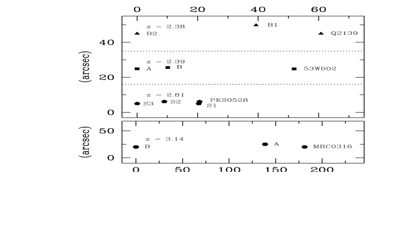
Figure 6: Relative positions of galaxies in four high-redshift groups discovered in Ly$\alpha\,$searches. Each group has been rotated so that the principal axis is horizontal in the figure, and the groups have been offset from one another vertically. Note the different scale of the lower plot.

To quantify the degree of alignment of each group we have measured the smallest internal angle $\delta_{L}$ of the triangle defined by the three objects in each group (for the PKS 0528-250 field at z=2.81 we used the position of S1 for the DLA absorber, rather than the position of the quasar sightline through the absorber). The measured angles are, from top to bottom in the figure, $\delta_{L}=7.0^{\circ},1.0^{\circ},5.8^{\circ},2.1^{\circ}$. The average value of the angle $\delta_{L}=4.0^{\circ}$ is certainly very suggestive of filamentariness in the distribution of galaxies at high redshift. It is also notable that the sizes of the groups range over an order of magnitude. In the computer simulations filaments are seen at all scales (e.g. Evrard et al. 1994). We do not suggest that every high-redshift group of three or four galaxies discovered will exhibit a similar degree of alignment, but rather that filamentary networks akin to those seen in the simulations may become visible as larger samples of high-redshift galaxies with denser sampling become available. The phenomenon might provide a useful discriminant for models of structure formation.

References

- [1996] Aragón-Salamanca A., Ellis R. S., O’Brien K. S., 1996, MNRAS 281, 945
- [1991] Bergeron J., Boissé P., 1991, A&A 243, 344
- [1996] Djorgovski S. G., Pahre M. A., Bechtold J., Elston R., 1996, Nature 382, 234
- [1996] Ebbels T. M. D., Le Borgne J.-F., Pellò R., Ellis R. S., Kneib J.-P., Smail I., Sanahuja B., 1996, MNRAS 281, L75
- [1994] Evrard A. E., Summers F. J., Davis M. 1994, ApJ 422, 11
- [1997] Fynbo J., Møller P., Warren S. J., 1997, in preparation
- [1996] Francis P. J., Woodgate B. E., Warren S. J., et al., 1995, ApJ 457, 490
- [1996] Ge J, Bechtold J., Walker C., Black J. H., 1997, ApJ 486, 727
- [1996] Giavalisco M., Steidel C. C., Macchetto F. D., 1996, ApJ 470, 189
- [1995] Holtzman J. A., Burrows C. J., Casertano S., et al., 1995, PASP 107, 1065
- [1997] Hook R. N., Fruchter A. S., 1997, ADASS VI, eds Hunt G., Payne H. E. (ASP Conf. Ser. 125), p. 147
- [1996] Katz N., Weinberg D. H., Hernquist L., Miralda-Escudé J., 1996, ApJ 457, L57
- [1991] Lanzetta K. M., Wolfe A. M., Turnshek D. A., Lu L., Mc Mahon R. G., Hazard C., 1991, ApJS 77, 1
- [1997] Le Brun V., Bergeron J., Boissé P., Deharveng J. M., 1997, A&A 321, 733
- [1996] Le Fèvre O., Deltorn J. M., Crampton D., Dickinson M., 1996, ApJ 471, L11
- [1991] Lowenthal J.D., Hogan C.J., Green R.F., Caulet A., Woodgate B.E., Brown L., Foltz C.B., 1991, ApJ 377, L73
- [1997] Lowenthal J.D., Koo D. C., Guzmán R., et al., 1997, ApJ 481, 673
- [1996] Madau P., Ferguson H. C., Dickinson M. E., Giavalisco M., Steidel C. C., Fruchter A., 1996, MNRAS 283, 1388
- [1991] Møller P., Warren S. J., 1991, in The Space Distribution of Quasars, ed. Crampton D. (ASP Conf. Ser. 21), p. 96
- [1993] Møller P., Warren S. J., 1993, A&A 270, 43 (Paper I)
- [1996] Møller P., Warren S. J., 1996, in Cold gas at high redshift, eds. M.N. Bremer, P.P. van der Werf, H.J.A. Röttgering and C.L. Carilli, Kluwer Academic Publishers, p233
- [1996] Pascarelle S. M., Windhorst R. A., Driver S. P., Ostrander E. J., Keel W. C., 1996, ApJ 456, L21
- [1995] Pettini M., Smith L. J., Hunstead R. W., King D. L., 1994, ApJ 426, 79
- [1995] Pei Y. C, Fall S. M., 1995, ApJ 454, 69
- [1965] Schmidt M., 1965, ApJ 141, 1295
- [1991] Steidel C. C., Sargent W. L. W., Dickinson M., 1991, AJ 101, 1187
- [1992] Steidel C. C., Hamilton, D., 1992, AJ 104, 941
- [1994] Steidel C. C., Dickinson M., Persson S. E., 1994a, ApJ 437, L75
- [1994] Steidel C. C., Pettini M., Dickinson M., Persson S. E., 1994b, AJ 108, 2046
- [1996] Steidel C. C., Giavalisco M., Pettini M., Dickinson M., Adelberger K. L., 1996, ApJ 462, L17
- [1996] Valls-Gabaud D., 1993, ApJ 419, 7
- [1996] Warren S. J., Møller P., 1996, A&A 311, 25 (Paper II)
- [1986] Wolfe A. M., Turnshek D. A., Smith H. E., Cohen R. D., 1986, ApJS 61, 249
- [1995] Wolfe A. M., Lanzetta K. M., Foltz C. B., Chaffee F. H., 1995, ApJ 454, 698