Evidence for a $3\times 10^{8}\>{\rm M_{\odot}}$ black hole in NGC 7052
from HST observations of the nuclear gas disk

Abstract

We present a Hubble Space Telescope (HST) study of the nuclear region of the E4 radio galaxy NGC 7052, which has a nuclear disk of dust and gas. The Second Wide Field and Planetary Camera (WFPC2) was used to obtain $B$, $V$ and $I$ broad-band images and an H$\alpha$+[NII] narrow-band image. The images yield the stellar surface brightness profile, the optical depth of the dust, and the flux distribution of the ionized gas. The Faint Object Spectrograph (FOS) was used to obtain H$\alpha$+[NII] spectra at six different positions along the major axis, using a $0.26^{\prime\prime}$ diameter circular aperture. The emission lines yield the rotation curve of the ionized gas and the radial profile of its velocity dispersion. The observed rotation velocity at $r=0.2^{\prime\prime}$ from the nucleus is $V=155\pm 17\>{\rm km}\,{\rm s}^{-1}$. The Gaussian dispersion of the emission lines increases from $\sigma\approx 70\>{\rm km}\,{\rm s}^{-1}$ at $r=1^{\prime\prime}$, to $\sigma\approx 400\>{\rm km}\,{\rm s}^{-1}$ on the nucleus.

To interpret the gas kinematics we construct axisymmetric models in which the gas and dust reside in a disk in the equatorial plane of the stellar body, and are viewed at an inclination of $70^{\circ}$. It is assumed that the gas moves on circular orbits, with an intrinsic velocity dispersion due to turbulence (or otherwise non-gravitational motion). The latter is required to fit the observed increase in the line widths towards the nucleus, and must reach a value in excess of $500\>{\rm km}\,{\rm s}^{-1}$ in the central $0.1^{\prime\prime}$. The circular velocity is calculated from the combined gravitational potential of the stars and a possible nuclear black hole. Models without a black hole predict a rotation curve that is shallower than observed ($V_{\rm pred}=92\>{\rm km}\,{\rm s}^{-1}$ at $r=0.2^{\prime\prime}$), and are ruled out at $>99$% confidence. Models with a black hole of mass $M_{\bullet}=3.3^{+2.3}_{-1.3}\times 10^{8}\>{\rm M_{\odot}}$ provide an acceptable fit. The best-fitting model with a black hole adequately reproduces the observed emission line shapes on the nucleus, which have a narrower peak and broader wings than a Gaussian.

NGC 7052 can be added to the list of active galaxies for which HST spectra of a nuclear gas disk provide evidence for the presence of a central black hole. The black hole masses inferred for M87, M84, NGC 6251, NGC 4261 and NGC 7052 span a range of a factor $10$, with NGC 7052 falling on the low end. By contrast, the luminosities of these galaxies are identical to within $\sim\!25$%. Any relation between black hole mass and luminosity, as suggested by independent arguments, must therefore have a scatter of at least a factor $10$.

1 Introduction

Astronomers have been searching for direct evidence for the presence of black holes (BHs) in galactic nuclei for more than two decades. Initially, the only constraints on the central mass distributions of galaxies were obtained from ground-based stellar kinematical observations. More recently, the launch of the Hubble Space Telescope (HST) and the subsequent refurbishment in 1993 have provided an important increase in spatial resolution. Combined with new techniques for data analysis and dynamical modeling this has strengthened the stellar kinematical evidence for BHs in several quiescent galaxies (e.g., Kormendy et al. 1996a,b; van der Marel et al. 1997a; Cretton & van den Bosch 1998; Gebhardt et al. 1998). New tools for the detection of BHs were also developed. HST observations of the rotation velocities of nuclear disks of ionized gas provided accurate BH mass determinations for several active galaxies (e.g., Harms et al. 1994; Ferrarese, Ford & Jaffe 1996, 1998; Macchetto et al. 1997; Bower et al. 1998), while for other galaxies BHs were detected through VLBI observations of nuclear water maser sources (e.g., Miyoshi et al. 1995). The case for a BH in our own galaxy improved drastically through measurements of stellar proper motions exceeding $1000\>{\rm km}\,{\rm s}^{-1}$ in the central $0.1\>{\rm pc}$ (Genzel et al. 1997). There are now a total of 10—20 galaxies for which a nuclear dark mass, most likely a BH, has been convincingly detected. The combined results for these galaxies are summarized and reviewed in, e.g., Kormendy & Richstone (1995), Ford et al. (1998), Ho (1998), Richstone (1998), and van der Marel (1998). This sample is now large enough to study the BH mass distribution in galaxies, which is further constrained by ground-based stellar kinematical observations (Magorrian et al. 1998), HST photometry (van der Marel 1998) and quasar evolution (e.g., Haehnelt et al. 1998). Our understanding remains sketchy, but is consistent with a picture in which a majority of galaxies has BHs, and in which the BH mass $M_{\bullet}$ correlates with the luminosity or mass of the host spheroid.

In this paper we present and analyze HST data for the E4 galaxy NGC 7052. This galaxy is a radio source with a core and jet, but no lobes (Morganti et al. 1987). Ground-based optical images show a nuclear dust disk aligned with the major axis of the galaxy (Nieto et al. 1990). The physical properties of this disk were discussed by de Juan, Colina & Golombek (1996). In a previous paper (van den Bosch & van der Marel 1995; hereafter Paper I) we presented ground-based narrow-band imaging and long-slit spectroscopy obtained with the 4.2m William Herschel Telescope (WHT). These observations showed that there is also a rotating nuclear disk of ionized gas in NGC 7052. The gas has a steep central rotation curve, rising to nearly $300\>{\rm km}\,{\rm s}^{-1}$ at $1^{\prime\prime}$ from the center. However, the spatial resolution of the spectra was insufficient to convincingly detect a BH, due in part to the relatively large distance of NGC 7052 ($58.7\>{\rm Mpc}$; i.e., $1^{\prime\prime}=284.6\>{\rm pc}$). The velocity dispersion of the gas was found to increase from $\sigma\approx 70\>{\rm km}\,{\rm s}^{-1}$ at $1^{\prime\prime}$ from the center to $\sigma\approx 200\>{\rm km}\,{\rm s}^{-1}$ on the nucleus. We showed that this cannot be the sole result of rotational broadening, which would have predicted double-peaked line profile shapes that are not observed. Instead, the observed central increase in the line width must be at least partly intrinsic. The ground-based kinematics yield an upper limit of $\sim 10^{9}\>{\rm M_{\odot}}$ on the mass of any possible BH.

To improve the constraints on the presence of a central BH we obtained broad- and narrow-band images of NGC 7052 with the Second Wide Field and Planetary Camera (WFPC2) and spectroscopy with the Faint Object Spectrograph (FOS), both in the context of HST project GO-5848. We discuss the imaging and photometric analysis in Section 2, and the spectroscopy and kinematical analysis in Section 3. In Section 4 we construct dynamical models to interpret the results. With the high spatial resolution of these data we are able to better constrain the nuclear mass distribution, and we find that NGC 7052 has a BH with mass $M_{\bullet}=3.3^{+2.3}_{-1.3}\times 10^{8}\>{\rm M_{\odot}}$. We summarize and discuss our findings in Section 5. Some observational details are presented in an appendix.

We adopt $H_{0}=80\>{\rm km}\,{\rm s}^{-1}\>{\rm Mpc}^{-1}$ throughout this paper. This does not directly influence the data-model comparison for any of our models, but does set the length, mass and luminosity scales of the models in physical units. Specifically, distances, lengths and masses scale as $H_{0}^{-1}$, while mass-to-light ratios scale as $H_{0}$.

2 WFPC2 observations and photometric analysis

2.1 Setup and data reduction

We used the WFPC2 to obtain both broad- and narrow-band images of NGC 7052. The WFPC2 is described in detail by, e.g., Biretta et al. (1996). The observations took five spacecraft orbits in one ‘visit’. Telescope tracking was done in ‘fine lock’, with a RMS telescope jitter of $\sim\!3$ milli-arcsec (mas). The observing log is presented in Table 1. We obtained broad-band images with the filters F450W, F547M and F814W, corresponding roughly to Johnson $B$, $V$ and $I$. We also obtained narrow-band images with the ‘linear ramp filter’ (LRF), for which the central wavelength varies as function of position. This filter has a transmission curve with a FWHM of $\sim\!1.3$% of the central wavelength. By placing the target at a known position on the detector, we obtained images of the nuclear region around $6675$Å (‘on-band’; covering H$\alpha$+[NII]) and $6480$Å (‘off-band’). The WFPC2 has four chips, each with $800\times 800$ pixels. The $B$ and $I$ images were taken with the galaxy centered on the PC chip, yielding a pixel size of $0.046^{\prime\prime}$. The $V$ and LRF images were taken with the galaxy centered on one of the WF chips, yielding a pixel size of $0.100^{\prime\prime}$.

The images were calibrated by the HST calibration ‘pipeline’ maintained by the Space Telescope Science Institute (STScI). The standard reduction steps include bias subtraction, dark current subtraction and flat-fielding, as described in detail by Holtzman et al. (1995a). The pipeline does not flat-field LRF images, so we manually flat-fielded those using the flat-field for a broad-band filter with a comparable central wavelength (F675W). Three different exposures were taken with each filter, each with the target shifted by a small integer number of pixels. The different exposures for each filter were aligned, and then combined with simultaneous removal of cosmic rays and chip defects. This yields one final image per filter. The final images were corrected for the geometric distortion of the WFPC2, and constant backgrounds were subtracted, as measured at those regions of the detector where the galactic contribution is negligible.

To obtain an image of the H$\alpha$+[NII] emission one must subtract an off-band image from the on-band image. One option is to use the $V$ or $I$-band image (or an appropriate combination) as off-band image. These images have the advantage of high signal-to-noise ratio ($S/N$). However, the central wavelengths differ significantly from that of H$\alpha$+[NII], so the dust absorption in these images may not be the same as in the on-band image. Such differential dust absorption may be incorrectly interpreted as gas emission. To minimize differential dust absorption, we instead used the $6480$Å LRF image as off-band image. This off-band image was aligned with the on-band image, scaled to fit the on-band image at radii where the ionized gas flux is negligible, and subtracted from the on-band image.

The count-rates in the broad-band F450W, F547M and F814W images were calibrated to magnitudes in the Johnson $B$, $V$ and $I$ bands, respectively, as described in Holtzman et al. (1995b). The count-rates in the LRF images were calibrated to erg cm^-2 s^-1 using calculations with the SYNPHOT package in IRAF. These calculations used the LRF transmission curve parameterizations given in Biretta et al. (1996) and the spectral energy distribution around H$\alpha$+[NII] measured in Paper I. The flux calibration of the H$\alpha$+[NII] image was verified by comparing it to the results of our HST/FOS spectroscopy.

2.2 Morphology

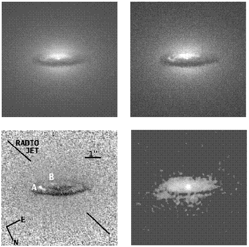
Figure 1: WFPC2 images of NGC 7052. From top-left to bottom right: $I$-band; $B$-band; $B-I$; and H$\alpha$+[NII]. Each panel covers a square region of $7.75^{\prime\prime}$. The $I$, $B$, and $B-I$ image were taken with the PC chip, yielding $0.046^{\prime\prime}$ pixels, and are shown with a linear strech. The darkest regions in the $B-I$ image have $B-I\approx 3.0$. The stellar distribution outside the region influenced by the disk has $B-I\approx 2.5$. The emission line image was constructed from narrow-band images taken with the WF chips, yielding $0.010^{\prime\prime}$ pixels. It has a sharply peaked flux distribution, but is shown here with a logarithmic stretch to show the low surface brightness features. The orientation on the sky and the position angle of the radio jet are indicated in the $B-I$ image. The regions labeled A and B are discussed in the text.

Figure 1 shows the reduced images, with from top-left to bottom-right, the $I$-band image, the $B$-band image, the $B-I$ image and the emission line image of H$\alpha$+[NII]. The most prominent feature in the broad-band images is the absorption by the dust disk. The morphology of the starlight in the central region resembles that of a cone emanating from the nucleus. Since no such structure is seen in the emission line image, we exclude the possibility that the cone is related to an ionization cone. Rather, the cone may indicate that the dust disk has a non-zero opening angle (such that its thickness increases with distance). However, without detailed modeling it is not possible to rule out alternative morphologies for the dust disk, such as a constant scale-height or ring morphology. The $B-I$ image shows the dust absorption more directly. The galaxy is reddest at the front edge of the disk ($B-I\approx 3.0$), because this is where the fraction of the starlight along the line of sight that is ‘eclipsed’ by the disk is largest. The dust lane is also visible in the H$\alpha$+[NII] image, but less prominently than in the broad-band images.

We have fitted by eye the outline of the dust disk in the $B-I$ image and the outline of the gas disk in the H$\alpha$+[NII] image. Both are well approximated by an ellipse, although the ionized gas has some additional filamentary extensions to the north and west. The fitted ellipses have a semi-major by semi-minor axis size of $1.94^{\prime\prime}\times 0.67^{\prime\prime}$ for the dust disk, and $2.08^{\prime\prime}\times 0.72^{\prime\prime}$ for the gas disk. The disks have very similar size, probably indicating a common origin. The inferred axial ratio is $q_{\rm disk}=0.35\pm 0.03$ for both components, where the error was estimated by eye. If we make the simplifying assumptions that both the dust and gas disks are circular, have negligible thickness, and reside in the equatorial plane, then the implied inclination is $i=\arccos q_{\rm disk}=(70\pm 2)^{\circ}$. This is in excellent agreement with the results of the models presented in paper I, which indicated $i=(70\pm 5)^{\circ}$.

The centroid of the stellar isophotes at large radii coincides with the observed peak surface brightness in the broad-band images to within the errors of $\sim\!0.02^{\prime\prime}$. This, combined with the point-like appearance of the ‘nucleus’ in the broad-band images, suggests that we may be seeing the center of the stellar distribution through the dust. In contrast with the case for NGC 4261 (Ferrarese, Ford & Jaffe 1996), we have found no evidence (to within the errors of $\sim\!0.04^{\prime\prime}$) that either the dust disk or the gas disk is offset from the galaxy center defined by the starlight. The principal axes of the stellar, gaseous and dust components are also well aligned. None of the components is aligned with the position angle of the radio jet in NGC 7052 (Morganti et al. 1987), as indicated in Figure 1. This has been found to be the case in more galaxies with nuclear gas disks (de Juan, Colina & Golombek 1996), although in other galaxies the alignment with the radio axis has been found to be quite good (e.g., NGC 4261 and M87; Ford et al. 1994; Ferrarese, Ford & Jaffe 1996).

The $B-I$ image shows two regions near the nucleus, labeled A and B, that are bluer ($B-I=2.0$—$2.5$) than most of the dust obscured region (which has $B-I=2.6$—$3.0$) and also than the main body of the galaxy. The blue color of these regions may be due to local star formation or to a contribution of [OIII]5007 emission to the $B$-band image (although no enhanced H$\alpha$+[NII] emission is seen at these positions). The region B is approximately aligned with the radio jet of NGC 7052, and could also be non-thermal optical emission from a jet knot. However, even the best available radio image of the jet (Morganti et al. 1987) has a resolution of more than $1$ arcsec, so it is unknown whether there is a radio knot at the position of the region B. Our ignorance of the exact nature of the regions A and B has no impact on our study of the nuclear mass distribution of NGC 7052.

2.3 The stellar luminosity density

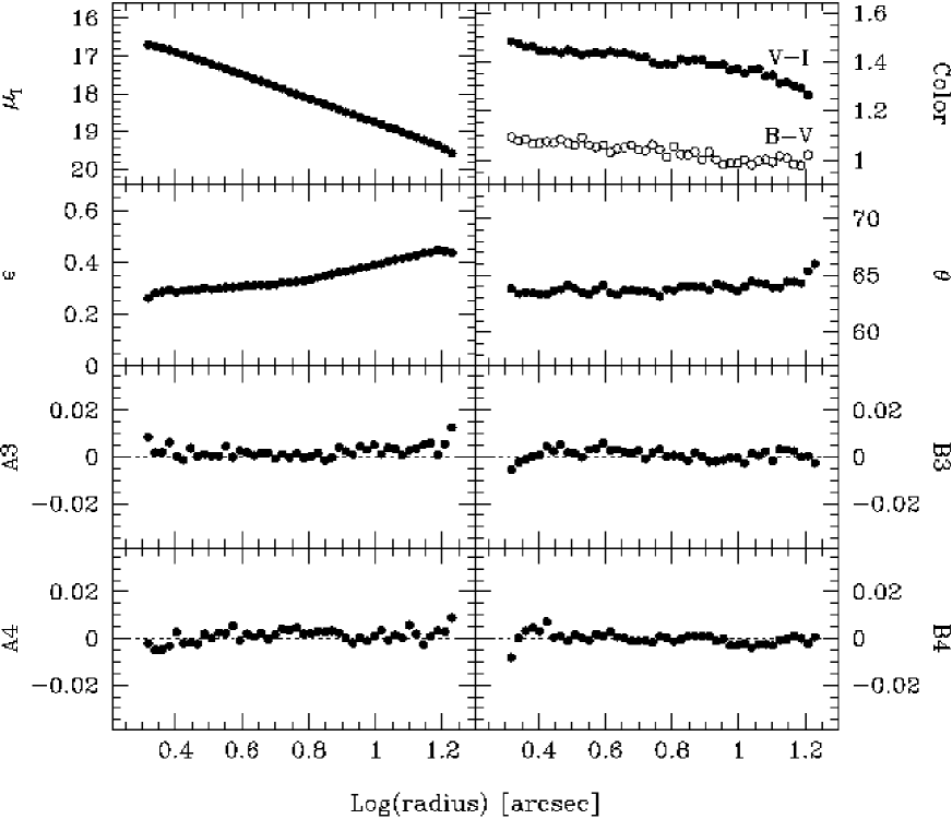
Figure 2: Isophotal parameters as function of major axis radius for the $I$-band image of NGC 7052, for the region outside the dust disk ($r>2.0^{\prime\prime}$). From left to right and top to bottom: the $I$-band surface brightness in mag arcsec^-2; the $B-V$ and $V-I$ color profiles; the ellipticity $\epsilon$; the major axis position angle $\theta$; and the third and fourth order Fourier sine ($A_{3}$ and $A_{4}$) and cosine ($B_{3}$ and $B_{4}$) terms that measure isophotal deviations from ellipses. The isophotal structure of NGC 7052 is not atypical for an elliptical galaxy.

The stellar surface brightness outside the dust distribution is best analyzed by fitting ellipses to the isophotes. We have done this with the software in the IRAF package STSDAS, which is based on the algorithm of Jedrzejewski (1987). Figure 2 shows the $I$-band surface brightness, the $B-V$ and $V-I$ colors, the ellipticity ($\epsilon$), the major axis position angle ($\theta$) and the amplitudes of the third and fourth order Fourier coefficients of the isophotes (describing deviations from pure ellipses), all as functions of radius along the major axis. Results are not shown for $r\lesssim 2.0^{\prime\prime}$, where dust absorption dominates the observed morphology.

The isophotal structure of NGC 7052 outside the dust disk is very regular. The third and fourth order Fourier coefficients are consistent with zero, indicating that the isophotes are accurately elliptical. No significant isophote twist is present. There is only a moderate increase in ellipticity, running from $\sim 0.3$ just outside the dust disk, to $\sim 0.4$ at the edge of the HST images ($r\sim 15^{\prime\prime}$).

To study the stellar surface brightness distribution at small radii, we consider the observed minor axis profile on the side of the galaxy where the dust absorption is smallest (i.e., upward in Figure 1). Figure 3 shows the $I$-band profile averaged over a $0.14^{\prime\prime}$ wide strip. The dust disk extends $\sim 0.67^{\prime\prime}$ along the minor axis. The observed profile outside this radius reflects the true stellar brightness profile, but at smaller radii the brightness has been decreased by dust absorption.

To model the stellar surface brightness we adopt a parameterization for the three-dimensional stellar luminosity density $j$. We assume that $j$ is oblate axisymmetric, that the isoluminosity spheroids have constant flattening $q$ as a function of radius, and that $j$ can be parameterized as

$$j(R,z)=j_{0}(m/a)^{-\alpha}[1+(m/a)^{2}]^{-\beta},\quad m^{2}\equiv R^{2}+z^{2}q^{-2}.$$ (1)

Here $(R,z)$ are the usual cylindrical coordinates, and $\alpha$, $\beta$, $a$ and $j_{0}$ are free parameters. When viewed at inclination angle $i$, the projected intensity contours are ellipses with axial ratio $q^{\prime}$, with $q^{\prime 2}\equiv\cos^{2}i+q^{2}\sin^{2}i$. The projected intensity for the luminosity density $j$ must be calculated numerically. In the following we adopt $i=70^{\circ}$, based on the observed shape of the dust and gas disks, and $q^{\prime}=0.7$, as appropriate for the region just outside the dust disk (cf. Figure 2). We neglect the slight increase in the observed ellipticity with radius.

The minor axis $I$-band profile does not strongly constrain the central cusp slope $\alpha$, because of the dust absorption at small radii. We therefore consider a one-parameter family of models with different $\alpha$. For any fixed $\alpha$, the remaining model parameters are determined by $\chi^{2}$ minimization to best fit the minor axis $I$-band profile outside the region influenced by dust (between $0.67^{\prime\prime}$ and $4.0^{\prime\prime}$). In the data-model comparison we use the projected surface brightness profile predicted by equation (1), convolved with the WFPC2 point-spread-function (PSF) and pixel size. The PSF convolution is important because the PSF wings extend to several arcseconds, despite the fact that the FWHM is only $0.1^{\prime\prime}$. Dotted curves in the top panel of Figure 3 show the predictions for $\alpha=0.1$, $0.2$, $0.3,\ldots,1.3$. The bottom panel shows the residuals for each fit, which must be attributed to dust absorption.

Models with larger values of $\alpha$ have more dust absorption, and therefore predict more reddening of the starlight. So to further constrain the models, and in particular $\alpha$, we consider the observed $B-I$ color. Figure 4 shows $B-I$ as function of minor axis distance, again averaged over a $0.14^{\prime\prime}$ wide strip centered on the nucleus. Outside the central arcsec there is a smooth color gradient, seen also in Figure 2. The colors and color gradients of NGC 7052 have values typical of elliptical galaxies. Color gradients such as seen in NGC 7052 are believed to be due to stellar population gradients (e.g., Kormendy & Djorgovski 1989). Extrapolation of the outer $B-I$ gradient in NGC 7052 into the center emphasizes the additional reddening due to dust absorption. The $B-I$ is largest at negative radii (downward in Figure 1), which are at the front side of the dust disk. The reddening at positive radii is more modest. The nucleus itself is slightly bluer than its surroundings (see also Figure 1). This may be an artifact due to differences in the PSFs for the $B$ and the $I$-band images, but it may also indicate a contribution of a nuclear non-thermal continuum or the presence of a central hole in the dust distribution.

To model the observed reddening we assume that the dust resides in the equatorial plane. Let the $z$-axis be oriented such that the observer sees the region $z>0$ in front of the dust disk, and let the $w$-axis be along the line-of-sight. The $I$-band surface brightnesses due to the stars in front of and behind the dust are, respectively,

$$I_{+}=\int_{z>0}j_{I}\>{\rm d}w,\qquad I_{-}=\int_{z<0}j_{I}\>{\rm d}w.$$ (2)

Here $j_{I}$ is the intrinsic $I$-band luminosity density, which we assume to be of the functional form given in equation (1). The observed $I$-band flux in pixel $i$ is

$${\widetilde{I}_{i}}={\widetilde{I}_{+,i}}+{\widetilde{I}_{-,i}}\exp[{-{\widehat{\tau}_{I,i}}}],$$ (3)

where the tildes denote convolution with the instrumental PSF and pixel size. The quantity $\widehat{\tau}$ is the ‘effective’ optical depth that the light in pixel $i$ has encountered. Similarly, the observed $B$-band flux in pixel $i$ is

$${\widetilde{B}_{i}}={\widetilde{B}_{+,i}}+{\widetilde{B}_{-,i}}\exp[{-{\widehat{\tau}_{B,i}}}].$$ (4)

Given the $I$-band image and a model for $j_{I}$, it is possible to make predictions for the $B$-band image that can be compared to the data. For a given $j_{I}$, we calculate ${\widetilde{I}_{+}}$ and ${\widetilde{I}_{-}}$ from equation (2). We then assume the stellar population gradient in $B-I$ to be given by the linear fit in Figure 4. Combined with ${\widetilde{I}_{+}}$ and ${\widetilde{I}_{-}}$ this yields predictions for ${\widetilde{B}_{+}}$ and ${\widetilde{B}_{-}}$ (neglecting the small differences in the PSFs for the $B$ and the $I$-band images). The observed $I$-band flux yields ${\widehat{\tau}_{I}}$ from equation (3). For galactic dust, $\tau_{B}/\tau_{I}=2.3347$ (Cardelli, Clayton & Mathis 1989). Assuming that this ratio also applies to the effective optical depths in NGC 7052, one obtains predictions for ${\widehat{\tau}_{B}}$. Combined with ${\widetilde{B}_{+}}$ and ${\widetilde{B}_{-}}$, equation (4) then yields the predicted $B$-band flux.

This scheme yields predictions $B_{\rm pred}$ for the $B$-band fluxes for any assumed value of the central cusp slope $\alpha$. These predictions can be compared to the observed fluxes $B_{\rm obs}$ using the quantity

$$\chi^{2}_{\alpha}=\sum_{i}\Biggl{(}{B_{{\rm pred},i}-B_{{\rm obs},i}\over\Delta B_{{\rm obs},i}}\Biggr{)}^{2}.$$ (5)

In the summation we use pixels for which the projected radius $[x^{2}+y^{2}]^{1/2}$ exceeds $0.2^{\prime\prime}$ (to exclude pixels that may be influenced by PSF differences between the $B$ and $I$-bands), and for which the radius $[x^{2}+(y/\cos i)^{2}]^{1/2}$ in the equatorial plane is less than $2.0^{\prime\prime}$ (to exclude regions where there is no dust). Also, the comparison is limited to only one side of the dust disk (the right half in Figure 1; this excludes the regions A and B which may be contaminated by [OIII] emission). This yields a total of 995 pixels. The resulting $\chi^{2}_{\alpha}$ is shown as function of $\alpha$ in the left panel of Figure 5. The minimum $\chi^{2}_{\alpha}$ is reached for $\alpha=0.5$. Formal $\Delta\chi^{2}$-statistics yield a very stringent constraint on the cusp steepness ($0.45\lesssim\alpha\lesssim 0.65$ at $99.73$% confidence). However, we are reluctant to accept this constraint at face value; many assumptions underly our approach, and even the minimum $\chi^{2}_{\alpha}$ is large for the number of degrees of freedom. Instead, we prefer to be conservative, and do not wish to rule out any model with $0.0\leq\alpha\lesssim 1.0$ solely on the basis of $\chi^{2}_{\alpha}$.

It is unphysical to find $B_{\rm obs}<{\widetilde{B}_{+}}$ in a given pixel; this is not even possible for infinite optical depth. Nonetheless, one may expect a small fraction of the pixels to have $B_{\rm obs}<{\widetilde{B}_{+}}$, due to the effects of Poisson noise. The right panel in Figure 5 shows the fraction of all pixels that has $B_{\rm obs}<{\widetilde{B}_{+}}$. This fraction grows rapidly with increasing $\alpha$, and becomes unacceptable for $\alpha\gtrsim 0.8$. We therefore conclude overall from our analysis of the reddening that $\alpha\lesssim 0.8$, with a best fit for $\alpha=0.5$.

Many groups have used the HST to study the surface brightness profiles of elliptical galaxies (e.g., Crane et al. 1993; Jaffe et al. 1994; Carollo et al. 1997; Faber et al. 1997). Faber et al. discuss the results for 61 galaxies, using the so-called ‘NUKER law’ parameterization for the projected surface brightness profiles (Byun et al. 1996). To enable a comparison with their results we have fitted NUKER laws to the projected intensity profiles of our models over the region $0.1^{\prime\prime}<r<10^{\prime\prime}$. Figure 6 shows the central projected intensity slope $\gamma$ of the NUKER law profile, as function of the central luminosity density slope $\alpha$ of our models. At asymptotically small radii one would expect $\gamma=\max(0,\alpha-1)$, but we find $\gamma>\max(0,\alpha-1)$ at the radii observable with HST (consistent with the findings of Gebhardt et al. 1996). The V-band absolute magnitude of NGC 7052 is $M_{V}=-22.15$. Faber et al. find that elliptical galaxies can be classified in two groups according to their surface brightness profiles, and that all galaxies in their sample with $M_{V}<-22$ can be classified as so-called ‘core galaxies’. The maximum $\gamma$ for the 25 core galaxies in their sample is $0.25$. It is therefore reasonable to assume that NGC 7052 also is a core galaxy with $\gamma\lesssim 0.25$, which implies that $\alpha\lesssim 1.0$, (cf. Figure 6). The NUKER law slope for $\alpha=0.5$ is $\gamma=0.09$, which is equal to the average for all the core galaxies in the Faber et al. sample. The constraints on $\alpha$ in NGC 7052 inferred from our WFPC2 images are therefore consistent with our understanding of elliptical galaxies as a class.

In the following we adopt the model with $\alpha=0.5$ as our ‘standard model’. The remaining parameters of this model are $\beta=0.96$, $a=1.10^{\prime\prime}$ and $j_{0}=14.8\>{\rm L_{\odot}}\>{\rm pc}^{-3}$ ($I$-band), which best fit the surface brightness profile at large radii. We restrict much of the following discussion to our standard model, but return to models with other values of $\alpha$ in Section 4.4. In particular, we show there that changes in the value of $\alpha$ cannot remove the need for a BH in NGC 7052.

2.4 The ionized gas disk

Figure 7 shows the H$\alpha$+[NII] flux along the major axis, the intermediate axis and the minor axis of the gas disk, respectively. The left panel shows the PSF profile for comparison. The flux distribution is sharply peaked towards the nucleus. However, the peak is broader than the PSF, so there is no evidence for an unresolved nuclear point source.

For use in Section 4 we require a model for the flux distribution. Given the lack of information on the distribution of the ionized gas along the line of sight, we assume that it resides in an infinitesimally thin circular disk in the equatorial plane of the galaxy, and we parameterize the H$\alpha$+[NII] flux $F(R)$ as a truncated double exponential:

$$F(R)=\cases{F_{1}\exp(-R/R_{1})+F_{2}\exp(-R/R_{2}),&$(R\leq{\bar{R}})$ ,\cr 0,&$(R>{\bar{R}})$ .\cr}$$ (6)

Observational information on the H$\alpha$+[NII] flux is available not only from the WFPC2 image, but also from the spectra obtained with the FOS (Section 3) and the WHT (Paper I). The best-fit parameters in equation (6) were determined using $\chi^{2}$ minimization to optimize the fit to all observational constraints on the emission line flux simultaneously. For the WFPC2 data we included only the one-dimensional profiles shown in Figure 7, rather than the entire two-dimensional image. Convolutions with the PSF and pixel and/or aperture size for each setup were properly taken into account.

The predictions of the best-fit model are shown as solid curves in Figure 7. The overall fit to the data is satisfactory, and our simple model is sufficient for the dynamical interpretation of the gas kinematics in Section 4. Nonetheless, two remarks must be made. First, the model is axisymmetric, so the features in the data that are not symmetric with respect to the nucleus (e.g., the bump at $\sim-1.0^{\prime\prime}$ along the major axis) cannot be reproduced. Second, there is some inconsistency between the central fluxes in the different data sets. The predicted and observed fluxes for the spectra are shown in Figure 11. The HST/FOS fluxes suggest a more sharply peaked flux distribution than the WFPC2 and WHT data, and our best fit model is a compromise between all the data. Our model therefore overpredicts the central flux measured in the WFPC2 data. The parameters of the best-fit model are: $R_{1}=0.032^{\prime\prime}$, $R_{2}=0.84^{\prime\prime}$, ${\bar{R}}=2.02^{\prime\prime}$, and $F_{1}/F_{2}=140$. The value of $F_{1}$ is not important for our models, but only sets the absolute normalization of the flux. The absolute calibration of our data is most accurate for the HST/FOS spectra, from which we derive $F_{1}=3.2\times 10^{-12}$ erg cm^-2 s^-1 arcsec^-2.

3 FOS observations and kinematical analysis

3.1 Setup and data reduction

We obtained spectra of NGC 7052 in visits on September 7, 1995 and August 18, 1996, using the red side detector of the HST/FOS. The instrument is described in detail in Keyes et al. (1995). The COSTAR optics corrected the spherical aberration of the HST primary mirror. The G570H grating was used in ‘quarter-stepping’ mode, yielding spectra with 2064 pixels covering the wavelength range from 4569 Å to 6818 Å. All spectra were obtained with a $0.26^{\prime\prime}$ diameter circular aperture (the FOS 0.3 aperture).

Each visit consisted of seven spacecraft orbits, with each orbit having $54$ minutes of target visibility time followed by $42$ minutes of Earth occultation. The first two orbits in each visit were used for target acquisition. Subsequent orbits were used to obtain spectra at various positions near the nucleus. Periods of Earth occultation were used to obtain wavelength calibration spectra of the internal arc lamp. In part of the last orbit of each visit the FOS was used in a special mode to obtain an image of the central part of NGC 7052, to verify the telescope pointing.

We performed the target acquisition in each visit through a ‘peak-up’ on a nearby star (magnitude $V=17.4$; coordinates in the HST Guide Star system: RA $=$ 21h 18m 32.46s, $\delta=26^{\circ}\,26^{\prime}\,57.6^{\prime\prime}$), followed by a telescope slew to the galaxy center (the dust in NGC 7052 prevents a peak-up directly on the galaxy center itself). Guided by simulations (van der Marel 1995), we used a non-standard 5-stage peak-up sequence with a predicted accuracy (in a noise-free situation) of $0.026^{\prime\prime}$ along each axis of the internal $(X,Y)$ coordinate system of the FOS. The position of the galaxy center with respect to the peak-up star was determined from the WFPC2 images before the spectroscopic observations: $\Delta{\rm RA}=0.6130$s and $\Delta\delta=-7.796^{\prime\prime}$. Systematic errors in the measurement of this offset and in the accuracy with which a slew of this size can be performed are $\lesssim 0.01^{\prime\prime}$. As for the WFPC2 imaging, telescope tracking during the observations was done in ‘fine lock’, with a RMS telescope jitter of $\sim\!3$ mas.

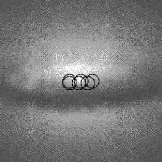
Figure 8: Aperture positions for the HST/FOS spectra, overlaid on the HST/WFPC2 $I$-band image of NGC 7052. All observations were obtained with the circular FOS 0.3 aperture, which has a diameter of $0.26^{\prime\prime}$. Table 2 lists various pieces of information about the spectra. The orientation of the image is the same as in Figure 1.

Galaxy spectra were obtained on the nucleus and along the major axis. Target acquisition uncertainties and other possible systematic effects may cause the aperture positions to differ from those commanded to the telescope. We therefore determined the aperture positions from the data themselves, using the target acquisition data, the ratios of the continuum and emission-line flux as observed through different apertures, and the FOS images obtained at the end of each visit. We describe this analysis in Appendix A. Table 2 lists the inferred aperture positions for all observations, as well as the exposure times. We give the positions in an $(x,y)$ coordinate system that is centered on the galaxy, and has its $x$-axis along the galaxy major axis (sky position angle $63.5^{\circ}$). The aperture positions are accurate to $\sim\!0.02^{\prime\prime}$ in either direction. Figure 8 shows the aperture positions overlaid on the WFPC2 $I$-band image.

Most of the necessary data reduction steps are performed by the HST calibration pipeline, including flat-fielding and absolute sensitivity calibration. The wavelength calibration provided by the pipeline is not accurate enough for our project, so we performed an improved calibration using the arc lamp spectra obtained in each orbit, following the procedure described in van der Marel (1997c). The relative accuracy (between different observations) of the resulting wavelength scale is $\sim 0.04$Å ($\sim\!2\>{\rm km}\,{\rm s}^{-1}$). Uncertainties in the absolute wavelength scale are larger, $\sim\!0.4$Å ($\sim\!20\>{\rm km}\,{\rm s}^{-1}$), but influence only the systemic velocity of NGC 7052, not the inferred BH mass.

3.2 Gas kinematics

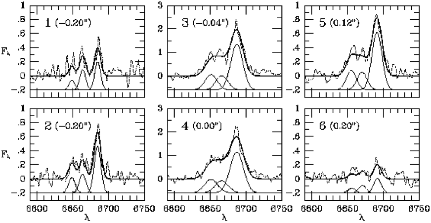
Figure 9: Dotted lines show the continuum-subtracted H$\alpha$+[NII] emission lines in the HST/FOS spectra of NGC 7052. The instrumental resolution is $4.15$Å FWHM, corresponding to a dispersion (FWHM/$2.355$) of $79\>{\rm km}\,{\rm s}^{-1}$. The spectra were smoothed with a Gaussian with a dispersion of $1$Å to reduce the noise. The abscissa is the observed vacuum wavelength in Å, and the ordinate is the flux observed through the $0.26^{\prime\prime}$ diameter aperture in $10^{-16}$ erg cm^-2 s^-1 Å^-1. A label in each panel indicates both the number of the observation, as defined in Table 2, and the major axis distance $x$ of the aperture center. Heavy solid curves are the fits to the spectra obtained under the assumption that all emission lines in a given spectrum are Gaussians with the same mean $V$ and dispersion $\sigma$, as described in the text. The individual Gaussian fits to [NII]$6548$, H$\alpha$ and [NII]$6583$ are displayed with a negative offset. The kinematical quantities $V$ and $\sigma$ are shown in Figure 10.

The H$\alpha$+[NII] lines are the only emission lines with a sufficiently high $S/N$ ratio for a kinematical analysis. To quantify the gas kinematics we fit the spectra under the assumption that each emission line is a Gaussian. The amplitude ratio H$\alpha$/[NII] is a free parameter in each fit, but [NII]$6583/6548$ is always fixed to 3, the ratio of the transition probabilities. We assume that all three lines in a given spectrum have the same mean velocity $V$ and velocity dispersion $\sigma$, and neglect the fact that the kinematics of the H$\alpha$ and [NII] lines may be slightly different (as suggested by Paper I). Figure 9 shows the observed spectra and the fits for all aperture positions.

The observed emission lines are not perfectly fit by Gaussians: they have a narrower core and broader wings. We discuss the line shapes in Section 4.2. For now we restrict the discussion to the Gaussian fit parameters $V$ and $\sigma$, which are listed with their formal errors in Table 2 (note that the mean and dispersion of the best-fitting Gaussian are well-defined and meaningful quantities, even if the lines themselves are not Gaussians). The systemic velocity of NGC 7052 (which was subtracted from the velocities in Table 2) was determined from the observed mean velocities by including it as a free parameter in the models discussed below, which yields $v_{\rm sys}=4705\pm 10\>{\rm km}\,{\rm s}^{-1}$. This is consistent with the velocity $v_{\rm sys}=4675\pm 45\>{\rm km}\,{\rm s}^{-1}$ inferred from the absorption lines in the HST spectra, and also with the literature value of $v_{\rm sys}=4710\pm 36\>{\rm km}\,{\rm s}^{-1}$ (Di Nella et al. 1995).

Figure 10 shows the kinematical quantities inferred from the FOS data as function of major axis distance. The figure also shows the kinematics inferred (in similar fashion using single-Gaussian fits) from the major axis ground-based spectra presented in Paper I. The line widths increase strongly towards the nucleus, similar to what has been found for other galaxies with nuclear gas disks (e.g., Ferrarese, Ford & Jaffe, 1996; Macchetto et al. 1997; Bower et al. 1998). As compared to the ground-based NGC 7052 data, the rotation curve inferred from the HST data is twice as steep, and the emission lines observed on the nucleus are twice as broad. To interpret these results we construct dynamical models for the gas motions.

4 The nuclear mass distribution

4.1 Dynamical models

Our models for the gas kinematics are similar to those employed in Paper I. The galaxy model is axisymmetric, with the stellar luminosity density $j(R,z)$ chosen as in Section 2.3 to fit the available surface photometry. We use our standard model for $j(R,z)$, unless otherwise specified. The stellar mass density $\rho(R,z)$ follows upon specification of a mass-to-light ratio $\Upsilon$. The gas resides in an infinitesimally thin disk in the equatorial plane of the galaxy, and has the circularly symmetric flux distribution $F(R)$ given in Section 2.4. The galaxy and the gas disk are viewed at an inclination $i$. The mean motion of the gas is characterized by circular orbits. The circular velocity $V_{\rm c}(R)$ is calculated from the combined gravitational potential of the stars and a nuclear BH of mass $M_{\bullet}$. The line-of-sight velocity profile (VP) of the gas at position $(x,y)$ on the sky is a Gaussian with dispersion $\sigma_{\rm gas}(R)$ and mean $V_{\rm c}(R)\sin i$, where $R^{2}=x^{2}+(y/\cos i)^{2}$ is the radius in the disk. The velocity dispersion of the gas is assumed to be isotropic, with contributions from thermal and non-thermal motions: $\sigma_{\rm gas}^{2}=\sigma_{\rm th}^{2}+\sigma_{\rm turb}^{2}$. We refer to the non-thermal contribution as ‘turbulent’, although we make no attempt to describe the underlying physical processes. It was concluded in Paper I that the intrinsic dispersion of the gas in NGC 7052 increases towards the nucleus, and it is sufficient here to parameterize $\sigma_{\rm turb}$ through:

$$\sigma_{\rm turb}(R)=\sigma_{0}+[\sigma_{1}\exp(-R/R_{\rm t})],$$ (7)

where $R$ is the radius in the disk. The predicted VP for any given observation is obtained through flux weighted convolution of the intrinsic VPs with the PSF of the observation and the size of the aperture. The convolutions are described by the semi-analytical kernels given in Appendix A of van der Marel et al. (1997b), and were performed numerically using Gauss-Legendre integration. A Gaussian is fit to each predicted VP for comparison to the observed $V$ and $\sigma$.

In a spectrograph, light at different positions in the aperture is detected at slightly different wavelengths. This induces line broadening, as well as small velocity shifts if the light is not distributed symmetrically within the aperture. Instrumental broadening also results from the finite size of a detector resolution element, and from the broadening due to the grating itself. For each observation we calculated the instrumental line spread function due to these effects as in Appendix B of van der Marel et al. (1997b). The resulting corrections on the predicted VPs and kinematical quantities were included in the models, but are not large ($\lesssim 6\>{\rm km}\,{\rm s}^{-1}$ for the inferred mean velocities).

Five free parameters are available to optimize the fit to the observed gas kinematics: $M_{\bullet}$, $\Upsilon$, and the parameters $\sigma_{0}$, $\sigma_{1}$ and $R_{\rm t}$ that describe the radial dependence of the turbulent dispersion. The temperature of the gas is not an important parameter: the thermal dispersion for $T\approx 10^{4}{\rm K}$ is $\sigma_{\rm th}\approx 10\>{\rm km}\,{\rm s}^{-1}$, and is negligible with respect to $\sigma_{\rm turb}$ for all plausible models. We define a $\chi^{2}$ quantity that measures the quality of the fit to the kinematical data. The best-fitting model is found by minimizing $\chi^{2}$ using a ‘downhill simplex’ minimization routine (Press et al. 1992).

Figure 11 shows the data that we have used in the definition of $\chi^{2}$, namely the new FOS data and the ground-based major and minor axis WHT data presented in Paper I. The latter were obtained in FWHM seeing of $0.57^{\prime\prime}$ and $0.84^{\prime\prime}$, respectively. Rotation velocity and velocity dispersion measurements were both included in the fit, yielding a total of 44 data points. The WHT data show some features that are in contradiction with the assumption of perfect axisymmetry: the velocity dispersion profiles along both the major and minor axes are not quite symmetric, and there is a small amount of rotation along the minor axis. This implies that the models can never fit the WHT measurements to within their formal errors, which are significantly smaller than those for the FOS data (a result of higher $S/N$). However, the models will automatically search for the best fit to the average of the measurements at positive and negative radii. We do not believe that this compromises our ability to infer the nuclear mass distribution of NGC 7052 with axisymmetric models. However, one complication is the weighting of data with its formal errors in the usual definition of $\chi^{2}$. This causes the minimization routine to assign disproportionate priority to features in the WHT data that it can never fit, while neglecting the fit to the FOS data. This is not desirable, because the FOS data have higher spatial resolution, and therefore contain more information on the mass distribution at small radii. To ensure that the FOS and WHT data receive roughly equal weight in the fitting process, we artificially assigned all WHT data points an error of $22.5\>{\rm km}\,{\rm s}^{-1}$ in the definition of $\chi^{2}$, equal to the median error for the HST data points. Although somewhat artificial, we have found that this works well in practice. It does mean that the resulting $\chi^{2}$ cannot be used for the calculation of confidence intervals on the best-fitting model parameters. We realize this, and therefore calculate in Section 4.3 confidence intervals on $M_{\bullet}$ on the basis of a statistic that only uses the FOS observations (for which the errors were taken as observed).

4.2 The best-fit model

The curves in Figure 11 show the predictions of the model that provides the overall best fit to the data. Its parameters are: $M_{\bullet}=3.3\times 10^{8}\>{\rm M_{\odot}}$, $\Upsilon=6.3$ (in $I$-band solar units), $\sigma_{0}=60\>{\rm km}\,{\rm s}^{-1}$, $\sigma_{1}=523\>{\rm km}\,{\rm s}^{-1}$ and $R_{\rm t}=0.11^{\prime\prime}$. This model adequately reproduces all the important features of the kinematical data, including the rotation curve slope and the nuclear velocity dispersion inferred from the HST data. The fit of our flux distribution model (equation [6]) to the observed fluxes (top panel of Figure 11) was discussed already in Section 2.4.

The circular velocity curve $V_{\rm c}(R)$ of a model with a BH has a minimum that is non-zero (for our best-fit model the minimum of $V_{\rm c}(R)\sin i$ is $180\>{\rm km}\,{\rm s}^{-1}$). Intrinsically, no gas moves slower than this, although gas for which only a fraction of the orbital velocity is observed along the line of sight may be observed at lower velocities. Hence, there is a tendency for models with a BH to predict double-peaked line profiles for observations on the nucleus, with the peaks at $|v|\approx[V_{\rm c}(R)]_{\rm min}\sin i$, corresponding to gas seen moving towards and away from the observer on either side of the nucleus. However, a significant intrinsic dispersion for the gas will tend to ‘wash away’ the peaks. Our best-fit model has both a BH and a significant intrinsic velocity dispersion. It is therefore interesting to study whether its predicted line shapes are comparable to the observed ones. Figure 12b compares the predicted spectrum to the data for FOS observation #4 (see Table 2), which was obtained on the nucleus. The model does not predict double-peaked or flat-topped line profiles, but instead predicts profiles with a narrow core and broad wings, as seen in the observations. The predictions are acceptable, and fit better than Gaussian profiles (shown in Figure 12a for comparison). Similar results were obtained for the other FOS observations. The fits to the line shapes could conceivably be improved further by allowing the intrinsic velocity distribution in the disk at any given position to be non-Gaussian, but this is not something that we have explored. It is already clear that our best-fit model is consistent with the observed line shapes.

The observed velocity dispersion of the gas increases from $\sim\!70\>{\rm km}\,{\rm s}^{-1}$ at $1^{\prime\prime}$ from the nucleus, to $\sim\!400\>{\rm km}\,{\rm s}^{-1}$ as seen through the $0.26^{\prime\prime}$ diameter FOS aperture on the nucleus. In principle, one can get an increase in the observed velocity dispersion towards the nucleus even if there is no intrinsic gradient, through the effect of rotational broadening around a central BH. However, it was shown already in Paper I that a model with a BH and no intrinsic velocity dispersion gradient is unacceptable: such a model predicts double-peaked emission line shapes that are in contradiction with observations. We similarly find that such models fail to fit the HST data. Hence, the intrinsic velocity dispersion of the gas in NGC 7052 must increase towards the nucleus. Our best-fit model has a turbulent velocity dispersion that increases to values in excess of $500\>{\rm km}\,{\rm s}^{-1}$ in the central $0.1^{\prime\prime}$. We argue in Section 4.5 that this is not in contradiction with the assumption of bulk circular motion for the gas. Thus, the ionized gas in NGC 7052 has both a sharply increasing flux and a sharply increasing velocity dispersion towards the nucleus. It may be that this signifies the presence of a (partly unresolved) narrow-line region. There is no evidence for a broad-line region, because the increasing line width is not restricted to H$\alpha$, but is seen in the forbidden [NII] lines as well.

4.3 The allowed range of black hole masses

To determine the range of BH masses that provides a statistically acceptable fit to the data, we compare the predictions of models with different, fixed values of $M_{\bullet}$, but in which the remaining parameters are varied to optimize the fit. The radial dependence of the intrinsic velocity dispersion of the gas is essentially a free function in our models, so the observed velocity dispersion measurements can be fit equally well for all plausible values of $M_{\bullet}$. The observed ground-based rotation measurements can also be fit equally well for all plausible $M_{\bullet}$ (i.e., $\lesssim 10^{9}\>{\rm M_{\odot}}$; cf. Paper I), because for all such values the radius of the BH sphere of influence is smaller than the ground-based spatial resolution. Thus only the predictions for the HST rotation velocity measurements depend substantially on the adopted $M_{\bullet}$.

Figure 13 compares the predictions for the HST rotation measurements for three different models. The solid curve is the best-fit model. The dashed curves are models in which $M_{\bullet}$ was fixed a priori to $0$ and $1.0\times 10^{9}\>{\rm M_{\odot}}$, respectively. The error weighted mean of the three velocity observations at $0.2^{\prime\prime}$ from the center is $V=155\pm 17\>{\rm km}\,{\rm s}^{-1}$. The model without a BH predicts $V=92\>{\rm km}\,{\rm s}^{-1}$, and its rotation curve slope is thus too shallow. The model with $M_{\bullet}=1.0\times 10^{9}\>{\rm M_{\odot}}$ predicts $V=214\>{\rm km}\,{\rm s}^{-1}$, and its rotation curve slope is thus too steep.

To assess the quality of the fit to the HST rotation velocity measurements we define a new $\chi^{2}$ quantity, $\chi^{2}_{V}$, that measures the fit to these data only. Figure 14 shows $\chi^{2}_{V}$ as function of $M_{\bullet}$. At each $M_{\bullet}$, the parameters $\Upsilon$, $\sigma_{0}$, $\sigma_{1}$ and $R_{\rm t}$ are fixed almost entirely by the ground-based data and the HST velocity dispersion measurements. These parameters can therefore not be varied independently to improve the fit to the HST rotation velocity measurements. As a result, $\chi^{2}_{V}$ follows approximately a $\chi^{2}$ probability distribution with $N_{\rm df}=6-1=5$ degrees of freedom (there are six HST measurements, and there is one free parameter: $M_{\bullet}$). The expectation value for this distribution is $\langle\chi^{2}_{V}\rangle=5$. The best-fit model has $[\chi^{2}_{V}]_{\rm min}=3.8$, and is thus entirely consistent with the data. Horizontal lines in Figure 14 show the probability that a value equal to or smaller than indicated would be observed for a correct model. These lines show that the $68.3$% (i.e., 1-$\sigma$) confidence interval for $M_{\bullet}$ is $[2.5\,;\,5.0]\times 10^{8}\>{\rm M_{\odot}}$, the $90$% confidence interval is $[1.9\,;\,6.5]\times 10^{8}\>{\rm M_{\odot}}$, and the $99$% confidence interval is $[1.2\,;\,8.2]\times 10^{8}\>{\rm M_{\odot}}$. Models without a BH are ruled out at $>99$% confidence.

4.4 Dependence on cusp slope

In Sections 4.2 and 4.3 we analyzed the gas kinematics using our standard model for the stellar luminosity density, which has a central cusp slope $\alpha=0.5$ (cf. Section 2.3). To assess the dependence of the inferred BH mass on $\alpha$ we repeated the analysis for a range of other $\alpha$ values, namely $\alpha=0.0,0.1,0.2,0.3,\ldots,1.3$.

Changing $\alpha$ from its standard value leaves the quality of the fit to the gas kinematics virtually unchanged; when $\alpha$ is changed, $M_{\bullet}$ and $\Upsilon$ can be changed simultaneously in such a way as to maintain a similar circular velocity curve. The best-fit dynamical models for different values of $\alpha$ therefore all have a similar turbulent velocity dispersion profile, but different values of $\Upsilon$ and $M_{\bullet}$. The dependence of the mass-to-light ratio on $\alpha$ is not very strong; $\Upsilon$ decreases monotonically with $\alpha$, from $\Upsilon=6.8$ for $\alpha=0.0$ to $\Upsilon=5.2$ for $\alpha=1.3$. The dependence of $M_{\bullet}$ on $\alpha$ is more important in the present context, and is shown in Figure 15. This figure not only shows the best-fit $M_{\bullet}$ for each $\alpha$, but also the $68.3$%, $90$% and $99$% confidence intervals, determined using the approach of Section 4.3. The best-fit value of $M_{\bullet}$ decreases monotonically with $\alpha$, from $M_{\bullet}=3.9\times 10^{8}\>{\rm M_{\odot}}$ for $\alpha=0.0$ to $M_{\bullet}=1.8\times 10^{8}\>{\rm M_{\odot}}$ for $\alpha=1.3$. Models with larger values of $\alpha$ have more stellar mass near the center, and therefore do not need as large a BH mass to explain the observed rotation curve. However, the best-fit model does invoke a BH for all values of $\alpha$. Models without a BH always predict a rotation curve that is shallower than observed, and are ruled out with $>99$% confidence over the entire range $0.0\leq\alpha\leq 1.3$.

Independent constraints on $\alpha$ were presented in Section 2.3. If NGC 7052 follows the trends displayed by other elliptical galaxies, then its luminosity determines that it must be a core galaxy. This yields $\alpha\lesssim 1.0$. Furthermore, the observed $B$$-$$I$ color of the dust obscured region implies that $\alpha\lesssim 0.8$. If we assume that $\alpha=0.5$ is the most likely value for $\alpha$ (based on Figure 5), but that none of the values of $\alpha$ in the range $0.0\leq\alpha\lesssim 0.8$ can be ruled out, we obtain $M_{\bullet}=3.3^{+2.3}_{-1.3}\times 10^{8}\>{\rm M_{\odot}}$ at $68.3$% confidence.

4.5 Stellar kinematics

In Paper I we presented a single measurement $\sigma_{\ast}=266\pm 26\>{\rm km}\,{\rm s}^{-1}$ of the stellar velocity dispersion in NGC 7052, obtained from the summed spectrum over a $10^{\prime\prime}$ wide and $0.8^{\prime\prime}$ high region along the major axis. To interpret this measurement we constructed stellar dynamical models with a phase-space distribution function of the form $f(E,L_{z})$ (as in Paper I), for $\alpha=0.0,0.1,0.2,0.3,\ldots,1.3$, respectively. For each $\alpha$, the values of $\Upsilon$ and $M_{\bullet}$ were taken to be as determined by the best fit to the gas kinematics (as in Sections 4.2 to 4.4). The stellar dynamics of each model were projected onto the sky and binned to obtain a prediction $\sigma_{\rm pred}$ for the observed $\sigma_{\ast}$.

The predicted dispersion decreases monotonically from $\sigma_{\rm pred}=272\>{\rm km}\,{\rm s}^{-1}$ for $\alpha=0.0$ to $\sigma_{\rm pred}=245\>{\rm km}\,{\rm s}^{-1}$ for $\alpha=1.3$. This implies that the predictions are consistent with the data for all values of $\alpha$. This is an important consistency check on our models for the gas kinematics. In particular, it confirms that the assumption of circular orbits for the gas is reasonable. If the gas in NGC 7052 were to move at significantly sub-circular velocities, then our models for the gas kinematics would yield an underestimate of the true mass-to-light $\Upsilon$. When used in our stellar dynamical models, this anomalously low $\Upsilon$ would lead to an underprediction of the observed stellar velocity dispersion, which we do not find to be the case.

This result lends support to our treatment of the intrinsic velocity dispersion of the gas. In our models we assume that this dispersion is due to local turbulence in gas that has bulk motion along circular orbits. An alternative would be to assume that the gas resides in individual clouds, and that the observed dispersion of the gas is due to a spread in the velocities of individual clouds seen along the line-of-sight. However, in this scenario the gas would behave similarly as other point particles (e.g., stars), and would therefore rotate significantly slower than the circular velocity (due to asymmetric drift). Our models would then have produced an underestimate of $\Upsilon$, and with this $\Upsilon$ our stellar dynamical models would have underpredicted the observed stellar velocity dispersion. As mentioned, we do not find this to be the case. This adds to the fact that the inferred $V/\sigma$ for the gas is less than unity. If the observed gas dispersion were due to gravitational motion of individual clouds, this $V/\sigma$ would be in contradiction with the fact that both the gas and the dust appear to reside in flat disks.

4.6 Adiabatic black hole growth

HST observations of early-type galaxies have shown that central power-law surface brightness cusps are ubiquitous. One possible scenario for the formation of such cusps is through adiabatic BH growth into a pre-existing homogeneous core (Young 1980). Although this is not a unique explanation, it may well be the correct one. For the case of M87 it has been shown to be in perfect agreement with the dynamically determined BH mass (Young et al. 1978; Lauer et al. 1992). Furthermore, the assumption that the cusps in all core galaxies are due to adiabatic BH growth implies a BH mass distribution that is in excellent agreement both with results from well-studied individual galaxies and with predictions from quasar statistics (van der Marel 1998).

If we assume that the presence of a surface brightness cusp of slope $\alpha$ in NGC 7052 is due to adiabatic BH growth as envisaged by Young, then each value of $\alpha$ corresponds to a unique BH mass $M_{\bullet}$. We determined the dependence of $M_{\bullet}$ on $\alpha$ by fitting adiabatic BH growth models calculated with the software of Quinlan et al. (1995) to the surface brightness profiles that correspond to the luminosity density parameterization of equation (1). The result is shown in Figure 15. The BH mass thus inferred agrees at the $90$% confidence level with the BH mass inferred from the gas kinematics if $0.16\leq\alpha\leq 0.53$. This includes the value $\alpha=0.5$ of our standard model.

These results provide new evidence for the applicability of Young’s models to core galaxies. It should be noted though that this does not necessarily imply that the BHs in core galaxies grew adiabatically. If the BH was present even before the galaxy formed, the end product would be very similar (Stiavelli 1998).

5 Discussion and conclusions

We have presented HST observations of the nuclear gas and dust disk in the E4 radio galaxy NGC 7052. WFPC2 broad- and narrow-band images were used to constrain the stellar surface brightness profile, the optical depth of the dust, and the flux distribution of the ionized gas. We have built axisymmetric models in which the gas and dust reside in the equatorial plane, and in which the gas moves on circular orbits with an additional velocity dispersion due to turbulence (or otherwise non-gravitational motion). These models were used to interpret the ionized gas kinematics inferred from our new FOS spectra and from existing ground-based spectra. The models fit the observed central rotation gradient only if there is a central BH with mass $M_{\bullet}=3.3^{+2.3}_{-1.3}\times 10^{8}\>{\rm M_{\odot}}$. Models without a black hole are ruled out at $>99$% confidence.

The models provide an adequate fit to the available observations with a minimum number of free parameters. The assumptions that we make are similar to those that have been made in HST studies of other galaxies with nuclear gas disks. In several areas our models are in fact more sophisticated than some of the previous work. In particular: we use our multi-colour photometry in order to constrain the central cusp steepness of the stellar mass distribution; we explicitly take into account the contribution of the axisymmetric stellar mass distribution to the circular velocity of the gas, and we do not assume the rotation field to be purely Keplerian; we explicitly model the convolution with the HST/FOS PSF and the binning over the size of the aperture; we model the full line profile shapes, and fit the widths of the emission lines as well as their mean; and we fit Gaussians to the models as we do the data, to properly take into account the fact that Gaussian fits to lines that may be skewed or have broad wings yield biased estimate of the true moments.

Still, our models remain only an approximation to the true structure of NGC 7052. In particular: the thickness of the gas disk may not be negligible; the mean motion of the gas may not be circular; and the observed rotation curve may not perfectly reflect the intrinsic rotation curve, because of partial absorption of the emission line flux by dust. The limited sky coverage of the FOS spectra prevents a direct check on whether the gas motions in NGC 7052 are indeed circular. However, several consistency checks are available that may have signaled errors in our assumptions; none did. The stellar mass-to-light ratio and systemic velocity inferred with our models from the nuclear gas kinematics agree with those inferred from stellar kinematical measurements outside the region influenced by dust absorption. The best-fitting model for the gas kinematics reproduces the shapes of the emission lines on the nucleus, despite the fact that these shapes were not included as constraints in the fit. These agreements do not rule out a conspiracy of some sort, but they do make it less likely that the observed gas kinematics are the result of vastly non-circular motion, or have been strongly modified by dust absorption. Models of adiabatic BH growth for the stellar surface brightness cusp provide another successful check: the BH mass implied by these models is fully consistent with that inferred from the gas kinematics.

Figure 16 shows a scatter plot of $M_{\bullet}$ versus $B$-band spheroid luminosity $L_{B,{\rm sph}}$ for all galaxies with reasonably secure BH mass determinations (adapted from van der Marel 1998, with the addition of NGC 7052; all for $H_{0}=80\>{\rm km}\,{\rm s}^{-1}\>{\rm Mpc}^{-1}$). There is a trend of increasing $M_{\bullet}$ with increasing $L_{B,{\rm sph}}$, although it remains difficult to rule out that systematic biases play some role in this relation (van der Marel 1998). Besides NGC 7052, the other galaxies for which the BH detections are based on kinematical studies of nuclear gas disks with the HST are M87 (Harms et al. 1994; Macchetto et al. 1997), M84 (Bower et al. 1998), NGC 6251 and NGC 4261 (Ferrarese, Ford & Jaffe, 1998, 1996). The $M_{\bullet}$ in these galaxies are $3.2\times 10^{9}$, $1.4\times 10^{9}$, $6.6\times 10^{8}$ and $M_{\bullet}=4.9\times 10^{8}\>{\rm M_{\odot}}$, respectively. NGC 7052 falls at the low end of this range. The five galaxies with BH evidence from nuclear gas disks form a very homogeneous set. Each of these galaxies is a radio source and is morphologically classified as an elliptical. The luminosities are identical to within $\sim\!25$% ($\log L_{B}$ in the range $10.6$—$10.8$ for all five galaxies). By contrast, the black hole masses span a range of a factor $10$. The results for these galaxies therefore show that any relation between $M_{\bullet}$ and $L_{B,{\rm sph}}$ must have a scatter of at least a factor $10$, even if the comparison is restricted to galaxies of similar type.

Appendix A Aperture positions for the FOS observations

In the first FOS visit (September 1995) the instrument was commanded to obtain spectra on the nucleus and at $\pm 0.2^{\prime\prime}$ along the major axis, and in the second visit (August 1996) on the nucleus and at $\pm 0.16^{\prime\prime}$ along the major axis. To determine the actual aperture positions during the observations we make the simplifying assumption that the relative positions of the apertures during each visit were as intended, but that for each visit there is one absolute offset (corresponding to the difference between the actual position of the galaxy center and the telescope’s estimate of the galaxy center). This assumption is justified if there is little telescope drift during the observations (telescope drifts during a visit are usually small, $\lesssim 0.03^{\prime\prime}$, although larger drifts can sometimes occur; e.g., van der Marel et al. 1997b). We have determined the absolute offset for each visit using three different methods, based on: (i) the target acquisition data; (ii) the ratios of either the continuum or the emission-line intensity between observations at different positions; and (iii) the FOS image obtained at the end of each visit.

The final target acquisition stage on the peak-up star placed the 0.3 aperture at a $5\times 5$ grid on the sky with inter-point spacings of $0.052^{\prime\prime}$. The intensity at each position was measured, and the grid point with the highest intensity was adopted by the telescope as its estimate of the position of the star. The intensities for all 25 positions were returned to the ground, and could be interpolated post hoc to determine the actual position of the star, which is not generally exactly at a grid point. This yields a direct estimate of the absolute positional offset for each visit, under the assumption that target acquisition inaccuracies provide the dominant source of positional error.

Each galaxy spectrum yields the total intensity in the H$\alpha$+[NII] lines and in the surrounding continuum. We binned the intensities observed in the WFPC2 on-band and off-band images in $0.26^{\prime\prime}$ circular apertures, and determined the absolute positional offset that best reproduces the intensities observed in the spectra. This yields a second estimate of the absolute positional offset for each visit, but only for the component along the major axis (both the intensity distribution and the positioning of the apertures are aligned along the major axis, so any positional offset in the direction parallel to the minor axis yields little change in the predicted intensity ratios).

The FOS image obtained at the end of each visit provides a third estimate of the absolute positional offset. The telescope was commanded to position the 4.3 aperture (a square aperture of $3.66^{\prime\prime}\times 3.71^{\prime\prime}$) at its estimate of the galaxy center, and to record an image by stepping the diode array of the instrument along the aperture. This yields an image with $0.075^{\prime\prime}\times 0.081^{\prime\prime}$ pixels, with a point-spread-function equal to the size of one diode ($0.301^{\prime\prime}\times 1.291^{\prime\prime}$). We modeled the image for each visit by masking the WFPC2 $I$-band image with the aperture size, convolving it with the boxcar PSF of one diode, and determining the absolute positional offset that provides the best fit in a $\chi^{2}$ sense to the observed FOS image.

For each visit, the three different methods for determining the absolute positional offset yield results that are mutually consistent to within $0.02^{\prime\prime}$ in each coordinate. For the first spectroscopic visit we find $(\Delta x,\Delta y)=(0.00^{\prime\prime},0.01^{\prime\prime})$, and for the second visit $(\Delta x,\Delta y)=(-0.04^{\prime\prime},-0.02^{\prime\prime})$, where $(x,y)$ is the coordinate system used in Section 3.1.

Figure 3: The heavy solid line in the top panel is the observed $I$-band intensity profile along the minor axis, averaged over a $0.14^{\prime\prime}$ wide strip centered on the galaxy. The abscissa is the distance to the galaxy center, measured along the minor axis in the direction least affected by dust obscuration (‘upward’ in Figure 1). The dashed vertical line indicates the approximate extent of the dust disk. Dotted curves are predictions of models with the stellar luminosity density parameterization of equation (1), for $\alpha=0.1$, $0.2$, $0.3,\ldots,1.3$. Our standard model has $\alpha=0.5$, and is shown with a solid curve. At each fixed $\alpha$, the remaining model parameters were chosen to optimize the fit to the data outside the dust region (to the right of the dashed line). The models take PSF convolution and pixel binning into account. The bottom panel shows the residuals of each of the fits.

Figure 4: The $B-I$ color as function of minor axis distance, averaged over a $0.14^{\prime\prime}$ wide strip centered on the galaxy. Positive radii correspond to the upward direction in Figure 1. Dotted vertical lines indicate the approximate extent of the dust disk. The color variation outside the central arcsec is due to a radial stellar population gradient. The solid line provides a linear fit to this gradient, and is extrapolated into the disk region as a dashed line. The disk has its largest $B-I$ at negative radii, at the front side of the disk. The nucleus is slightly bluer than its surroundings, possibly due to a contribution from non-thermal continuum.

Figure 5: The left panel shows $\chi^{2}_{\alpha}$ as function of the intrinsic central cusp slope $\alpha$. The quantity $\chi^{2}_{\alpha}$ measures the quality of the fit to the observed $B$-band flux for the predictions obtained as described in the text. In essence, $\alpha$ fixes the optical depth of the dust in the $I$-band, and $\chi^{2}_{\alpha}$ measures how well this optical depth fits the observed reddening of the galaxy light. The right panel shows the fraction $f$ of pixels that has a smaller $B$-band flux than would be expected for infinite optical depth. Small values of $f$ can be attributed to Poisson noise, but large values indicate that the underlying model is incorrect. We conclude from the combined results in both panels that $\alpha\lesssim 0.8$ with a most likely value of $\alpha=0.5$.

Figure 6: The NUKER law fit parameter $\gamma$ as function of the parameter $\alpha$ of our models, when fit over the region between $0.1^{\prime\prime}$ and $10^{\prime\prime}$. The former measures the central logarithmic slope of the projected intensity, the latter the central logarithmic slope of the luminosity density. At asymptotically small radii the two are related according to $\gamma=\max(0,\alpha-1)$, as indicated by the dashed line.

Figure 7: Solid dots show the H$\alpha$+[NII] flux (in arbitrary units) as function of the distance $R$ from the center, measured from the WFPC2 emission-line image along the major axis, the intermediate axis, and the minor axis, respectively. The dotted curve in the left panel shows the WFPC2 PSF. The observed flux distribution is peaked towards the center, but is broader than the PSF, and thus resolved. The solid curves in each panel show the predictions of the best-fitting model with the flux distribution of equation (6), after convolution with the PSF and pixel size. The parameters of this model were chosen to simultaneously optimize the fit to the fluxes obtained from the WFPC2 data and those obtained from the FOS and ground-based spectra (see the top row of Figure 11). The flux distribution outside the central region is somewhat asymmetric, in particular along the major axis. This is not reproduced by the model, but the overall fit is satisfactory.

Figure 10: Mean velocity $V$ and velocity dispersion $\sigma$ in $\>{\rm km}\,{\rm s}^{-1}$ as function of major axis distance $x$ in arcsec, for Gaussian fits to the H$\alpha$+[NII] emission lines in NGC 7052. The solid points are the results obtained with the HST/FOS from observations with a $0.26^{\prime\prime}$ diameter aperture, as listed in Table 2. The actual fits to the spectra are shown in Figure 9. The connected symbols are the results obtained from the major axis ground-based WHT spectra presented in Paper I, obtained in $0.57^{\prime\prime}$ FWHM seeing. The kinematical gradients inferred from the higher spatial resolution HST data are significantly steeper.

Figure 11: Data-model comparison for the flux and kinematics of the ionized gas. Gaussian fits to the emission lines were used to obtain measurements of the total H$\alpha$+[NII] flux $I$ (in $10^{-14}$ erg cm^-2 s^-1 per aperture), the mean velocity $V$, and the velocity dispersion $\sigma$ (in $\>{\rm km}\,{\rm s}^{-1}$). From left to right, the observations are from the HST/FOS, with $0.26^{\prime\prime}$ diameter apertures aligned along the major axis, and from long-slit ground-based WHT observations along the major and minor axes, obtained with seeing FWHM of $0.57^{\prime\prime}$ and $0.84^{\prime\prime}$, respectively, and with $0.33^{\prime\prime}\times 0.8^{\prime\prime}$ apertures. The horizontal scale in the panels for the HST data is five times smaller than in the other panels. Errors for the WHT data are often smaller than the plot symbols. The curves in the top row are the predictions generated by our model for the intrinsic flux distribution of the gas (equation [6]). The curves in the bottom two rows are the predictions of our best-fit model for the gas kinematics, using our standard model for the stellar luminosity density ($\alpha=0.5$). The dynamical model has a BH of $3.3\times 10^{8}\>{\rm M_{\odot}}$, and provides an adequate fit.

Figure 12: The dotted line in each panel is the continuum-subtracted HST/FOS spectrum for observation #4 (see Table 2), which was obtained on the nucleus. The top panel shows the best-fit when each emission line is assumed to have a Gaussian shape (as in Figure 9). The individual fits to [NII]$6548$, H$\alpha$ and [NII]$6583$ are displayed with a negative offset. The bottom panel shows the fit to the spectrum when the shape and width of each line are chosen as predicted by the best-fit model (Figure 11), with the flux in each of the lines and the mean velocity chosen to optimize the fit to the data. The predicted line shapes have a narrower core and broader wings than a Gaussian. This fits the observations well, better than the Gaussians in the top panel. The gas in the model has a large intrinsic dispersion, so the predictions do not show a double-peaked profile, despite the presence of a $3.3\times 10^{8}\>{\rm M_{\odot}}$ BH.

Figure 13: Datapoints show the mean velocities $V$ (in $\>{\rm km}\,{\rm s}^{-1}$) inferred from Gaussian fits to the H$\alpha$+[NII] emission lines in the HST/FOS spectra. The solid curve shows the predictions for these data, for the model that provides the overall best fit to all available kinematical data (Figure 11). This model has $M_{\bullet}=3.3\times 10^{8}\>{\rm M_{\odot}}$. The long and short dashed curves shows the predictions of models that best fit the data when the BH mass is kept fixed at $M_{\bullet}=0$ and $M_{\bullet}=1.0\times 10^{9}\>{\rm M_{\odot}}$, respectively, yielding rotation curves that are either too shallow or too steep. Both models are ruled out at $>99$% confidence (cf. Figure 14). The predictions in this figure use our standard model for the stellar luminosity density ($\alpha=0.5$). Similar results are obtained for other values of $\alpha$.

Figure 14: Models were constructed with the BH mass fixed to the value shown along the abscissa. The remaining parameters in each model were chosen to optimize the fit to all available gas kinematical data (shown in Figure 11). The solid curve shows for each model thus obtained the quantity $\chi^{2}_{V}$ that measures the quality of the fit to the HST/FOS rotation velocity measurements (shown in Figure 13). This quantity follows a $\chi^{2}$ probability distribution with $N_{\rm df}=5$. Horizontal dashed lines at given values of $\chi^{2}_{V}$ show the probability that a value equal to or smaller than indicated would be observed for a correct model. The model without a BH is ruled out at $>99$% confidence. The predictions in this figure use our standard model for the stellar luminosity density ($\alpha=0.5$). Similar results are obtained for other values of $\alpha$ (cf. Figure 15).

Figure 15: BH mass $M_{\bullet}$ (in $\>{\rm M_{\odot}}$) as function of the central cusp slope $\alpha$ of the three-dimensional luminosity density. The heavy solid curve shows the $M_{\bullet}$ that best fit the gas kinematics. The thin dotted, dashed, and long-dashed curves show the 68.3%, 90% and 99% confidence intervals on $M_{\bullet}$ implied by the gas kinematics, respectively. The heavy long-dashed curve shows the relation between $M_{\bullet}$ and $\alpha$ implied by the assumption that the presence of a density cusp is due to adiabatic growth of a BH into a pre-existing homogeneous core. The horizontal arrows indicate the upper limits on $\alpha$ obtained from the observed $B$$-$$I$ color, and from the fact that a galaxy with the luminosity of NGC 7052 is probably a core galaxy. Our standard model has $\alpha=0.5$ and $M_{\bullet}=3.3\times 10^{8}\>{\rm M_{\odot}}$. Models without a BH are ruled out with $>99$% confidence for all values of $\alpha$ plotted here.

Figure 16: Measurements of BH mass $M_{\bullet}$ versus $B$-band spheroid luminosity $L_{B,{\rm sph}}$, for ‘secure’ BH detections inferred from: ($\circ$) ionized gas kinematics of nuclear disks; ($\bullet$) stellar kinematical studies; ($\times$) radio observations of water masers; ($\ast$) time variability of broad double-peaked Balmer lines. The $M_{\bullet}$ values are typically believed to be accurate to $|\Delta\log M_{\bullet}|\lesssim 0.3$. The dashed line shows the $M_{\bullet}$ for which the BH sphere of influence, $r_{\bullet}\simeq GM_{\bullet}/\sigma^{2}$, extends $0.1^{\prime\prime}$ at a distance of $10\>{\rm Mpc}$ ($\sigma$ is determined by $L_{B,{\rm sph}}$ through the Faber-Jackson relation). BHs below this line can be detected only in galaxies closer than $10\>{\rm Mpc}$, and in galaxies in which kinematical tracers can be observed at resolutions $<0.1^{\prime\prime}$ (e.g., water masers). This figure was adapted from figure 1a of van der Marel (1998), which also lists the references for the individual galaxies.

Table 1: HST/WFPC2 images: observational setup

filter	$\lambda_{0}$	$\Delta\lambda$	HST-ID	$T_{\rm exp}$	CCD	pixel
	(Å)	(Å)		(s)		(arcsec)
(1)	(2)	(3)	(4)	(5)	(6)	(7)
F450W	4445	925	4–6	1030	PC	$0.046$
F547M	5454	487	7–9	840	WF2	$0.100$
LRF(off-band)	6480	83	d–f	3600	WF3	$0.100$
LRF(on-band)	6675	85	a–c	3700	WF2	$0.100$
F814W	8269	1758	1–3	1470	PC	$0.046$

Note. — WFPC2 images of NGC 7052 were obtained with 5 different filters. The filter name is listed in column (1). LRF stands for ‘linear ramp filter’ (a filter with a tunable central wavelength). Column (2) and (3) list the central wavelength of the filter and the FWHM, as defined in Biretta et al. (1996). In the HST Data Archive, the observations have names of the form u2p9010$\ast$t. Column (4) identifies the $\ast$ in the Archive name for each observation. Column (5) lists the total exposure time per filter, which for each filter was divided over three different exposures. Column (6) lists the WFPC2 CCD on which the target was positioned, and column (7) lists the resulting pixel size.

Table 2: HST/FOS spectra: observational setup and gas kinematics

ID	date	HST-ID	position		$T_{\rm exp}$	$V$	$\Delta V$	$\sigma$	$\Delta\sigma$
			$x$ (arcsec)	$y$ (arcsec)	($s$)	km/s	km/s	km/s	km/s
(1)	(2)	(3)	(4)	(5)	(6)	(7)	(8)	(9)	(10)
1	Aug 96	b	$-0.20$	$-0.02$	2380	$-147$	36	184	31
2	Sep 95	d, f	$-0.20$	$0.01$	3830	$-156$	21	209	17
3	Aug 96	d	$-0.04$	$-0.02$	2380	$-39$	22	379	20
4	Sep 95	7	$0.00$	$0.01$	2370	$-42$	24	421	23
5	Aug 96	7, 9, f	$0.12$	$-0.02$	6220	$138$	21	315	19
6	Sep 95	9, b	$0.20$	$0.01$	4770	$164$	54	235	44

Note. — FOS spectra of NGC 7052 were obtained at six different aperture positions. Column (1) is the label for the spectrum used in the remainder of the paper. Column (2) lists the month in which the obervation was obtained. In the HST Data Archive, the observations in September 1995 have names of the form y2p9020$\ast$p; those in August 1996 have names of the form y2p9040$\ast$t. Column (3) identifies the $\ast$ in the Archive name for each observation. Columns (4) and (5) list the aperture position for each observation, determined as described in Appendix A. The $(x,y)$ coordinate system is centered on the galaxy, with the $x$-axis along the major axis (position angle $63.5^{\circ}$). Column (6) lists the exposure time. Columns (7)-(10) list the mean velocity $V$ and velocity dispersion $\sigma$ of the emission line gas, with corresponding formal errors, determined from Gaussian fits to the emission lines as described in the text.

References

- (1) Biretta, J. A., et al. 1996, WFPC2 Instrument Handbook, Version 4.0 (Baltimore: STScI)
- (2) Bower, G. A., et al. 1997, ApJL, 492, L111
- (3) Byun, Y.-I., et al. 1996, AJ, 111, 1889
- (4) Cardelli, J. A., Clayton, G. C., & Mathis, J. S. 1989, ApJ, 345, 245
- (5) Carollo, C. M., Franx, M., Illingworth, G. D., & Forbes D. A. 1997, ApJ, 481, 710
- (6) Crane, P., et al. 1993, AJ, 106, 1371
- (7) Cretton, N., & van den Bosch, F. C. 1998, ApJ, submitted
- (8) De Juan, L., Colina, L., & Golombek, D. 1996, A&A, 305, 776
- (9) Di Nella, H., Garcia, A. M., Garnier R., & Paturel G. 1995, A&A Supplement, 113, 151
- (10) Faber, S. M., et al. 1997, AJ, 114, 1771
- (11) Ferrarese, L., Ford H. C., & Jaffe W. 1996, ApJ, 470, 444
- (12) Ferrarese, L., Ford, H. C., & Jaffe W. 1998, ApJ, in preparation
- (13) Ford, H. C., et al. 1994, ApJ, 435, L27
- (14) Ford, H. C., Tsvetanov, Z. I., Ferrarese L., & Jaffe W. 1998, in Proceedings IAU Symposium 184 (Dordrecht: Kluwer Academic Publishers), in press [astro-ph/9711299]
- (15) Gebhardt, K., et al. 1996, AJ, 112, 105
- (16) Gebhardt, K., et al. 1998, AJ, submitted
- (17) Genzel, R., Eckart, A., Ott, T., & Eisenhauer, F. 1997, MNRAS, 291, 219
- (18) Harms, R. J., et al. 1994, ApJ, 435, L35
- (19) Haehnelt, M. G., Natarajan, P., & Rees M. J. 1998, MNRAS, submitted [astro-ph/9712259]
- (20) Ho, L. 1998, in Observational Evidence for Black Holes in the Universe, ed. S. K. Chakrabarti (Dordrecht: Kluwer Academic Publishers), in press [astro-ph/9803307]
- (21) Holtzman, J., et al. 1995a, PASP, 107, 156
- (22) Holtzman, J., et al. 1995b, PASP, 107, 1065
- (23) Jaffe, W., Ford, H. C., O’Connell, R. W., van den Bosch, F. C., & Ferrarese, L. 1994, AJ, 108, 1567
- (24) Jedrzejewski, R. I. 1987, MNRAS, 226, 747
- (25) Keyes, C. D., Koratkar, A. P., Dahlem, M., Hayes, J., Christensen, J., & Martin, S. 1995, FOS Instrument Handbook, Version 6.0 (Baltimore: Space Telescope Science Institute)
- (26) Kormendy, J., Djorgovski S. G. 1989, ARA&A, 27, 235
- (27) Kormendy, J., Richstone, D. 1995, ARA&A, 33, 581
- (28) Kormendy, J., et al. 1996a, ApJ, 459, L57
- (29) Kormendy, J., et al. 1996b, ApJ, 473, L91
- (30) Lauer, T. R., et al. 1992, AJ, 103, 703
- (31) Macchetto, F., Marconi, A., Axon D. J., Capetti, A., & Sparks W. 1997, ApJ, 489, 579
- (32) Magorrian, J., et al. 1998, AJ, submitted [astro-ph/9708072]
- (33) Miyoshi, M., et al. 1995, Nature, 373, 127
- (34) Morganti, R., Fanti, C., Fanti, R., Parma, P., & De Ruiter H. R. 1987, A&A, 183, 203
- (35) Nieto, J.-L., McClure, R., Fletcher, J. M., Arnaud, J., Bacon, R., Bender, R., Comte, G., & Poulain, P. 1990, A&A, 235, L17
- (36) Press, W. H., Teukolsky, S. A., Vetterling, W. T., & Flannery, B. P. 1992, Numerical Recipes (Cambridge: Cambridge University Press)
- (37) Quinlan, G. D., Hernquist, L., & Sigurdsson, S. 1995, ApJ, 440, 554
- (38) Richstone, D. 1998, in Proceedings IAU Symposium 184 (Dordrecht: Kluwer Academic Publishers), in press
- (39) Stiavelli, M. 1998, ApJ, 495, L91
- (40) van den Bosch F., & van der Marel R. P. 1995, MNRAS, 274, 884 (Paper I)
- (41) van der Marel, R. P. 1995, in Calibrating Hubble Space Telescope: Post Servicing Mission, eds., A. Koratkar, & C. Leitherer (Baltimore: Space Telescope Science Institute), 94
- (42) van der Marel, R. P., de Zeeuw, P. T., Rix, H.-W., & Quinlan, G.D. 1997a, Nature, 385, 610
- (43) van der Marel, R. P., de Zeeuw, P. T., & Rix, H.-W. 1997b, ApJ, 488, 119
- (44) van der Marel, R. P. 1997c, in The 1997 HST Calibration Workshop, eds., S. Casertano et al. (Baltimore: Space Telescope Science Institute), 443
- (45) van der Marel, R. P. 1998, in Proceedings IAU Symposium 186 (Dordrecht: Kluwer Academic Publishers), in press [astro-ph/9712076]
- (46) Young, P., Westphal, J. A., Kristian, J., Wilson, C. P., & Landauer, F. P. 1978, ApJ, 221, 721
- (47) Young, P. 1980, ApJ, 242, 1232