CMB ANISOTROPIES ON CIRCULAR SCANS

We address the problem of map-making with data from the Planck Surveyor High Frequency Instrument, with an emphasis on the understanding and modelling of instrumental effects, and in particular that of sidelobe straylight.

1 CMB mapping: A complex problem

The goal of a CMB satellite experiment as Planck Surveyor is a precise measurement of the temperature of the microwave sky, $T(\vec{n})$, as a function of direction $\vec{n}$. Data samples obtained with the experiment, however, are not directly quantities of interest, but rather depend in a complex way on sky temperature, on the instrument, and on the scan strategy.

1.1 Model of the measurement

The complex process of radiation detection and signal production which relates the detected signal to the temperature field on the sky may be modelled, for a given detector, by:

$$s(t)=h(t)\star\left[\eta(t)\int{\rm d}\nu\left(b(\nu,t)+H_{\rm filters}(\nu)\int_{(4\pi)}{\rm d}\Omega L_{\nu}({\rm R}_{t}(\vec{n}))T(\vec{n})\right)\right]+n(t)$$ (1)

$h(t)$ is a global impulse response of the detector and electronics, $\eta(t)$ is the detector efficiency, assumed to be (possibly) slowly time dependent, $H_{\rm filters}(\nu)$ is the transmission of the filters which set the frequency band of observation, $L_{\nu}(\vec{n})$ the frequency-dependent radiation pattern of the antenna (including all optical elements), ${\rm R}_{t}$ a time-dependent rotation which reflects the scan strategy, and $T(\vec{n})$ the temperature on the sky which one wishes to measure. Randomness in the process of detection (in photon arrivals, in electronic processes in the detectors) is represented by a noise term, $n(t)$. Finally, $b(\nu,t)$ is a self-emission term, due to radiation from instrumental parts (filters, slightly emissive mirrors…) impinging on the detectors.

We have written equation 1 in terms of continuous functions $s(t)$ and $T(\vec{n})$. In the following, we will use sampled and pixelised versions $s_{k}$ and $T_{p}$ when convenient. The problems of digitalisation and pixelisation, interesting by themselves, are left out of this discussion.

1.2 Data Processing

For optimal mapping of the CMB anisotropies, it is necessary to optimise mission parameters and options (optimisation of $h(t)$, $H_{\rm filters}(\nu)$, $L_{\nu}(\vec{n})$, ${\rm R}_{t}$…) as well as methods of data processing for recovering sky temperature maps from $s(t)$. The traditionnal approach of data processing in the context of CMB mapping consists in modelling the measurement as $s_{k}=A_{ki}y_{i}+n_{k}$ where $s_{k}$ is the vector of signal samples (measurements), $A$ a linear operator, $y_{i}=(T_{\rm pixel},X_{i})$ a vector of quantities to be determined from the data set, where $T_{\rm pixel}$ are sky temperatures in a set of pixels, and $X_{i}$ other quantities contributing to the signal. $n_{k}$ is a vector of noise realisations. If we assume that the noise autocorrelation matrix $N=\langle n\,n^{T}\rangle$ is known, then the inversion can be performed by computing the estimator:

$$\hat{y}=[A^{T}N^{-1}A]^{-1}\,A^{T}N^{-1}s_{k}$$ (2)

This method, in principle, produces the best unbiased estimate of the sky. It is in essence the one that has been used by the DMR team $\!{}^{{\bf?}}$. It suffers, however, from a few drawbacks that make it impractical for Planck. The first is the size of the linear system to be manipulated (a few million pixels on the sky, and a few billion samples per detector for a 1-year mission). The second is that it is not clear a priori that a relevant set of parameters $X_{i}$ can be identified and the remaining noise correlation matrix estimated reliably so that the measurement can be meaningfully modelled by a linear equation connecting $s_{k}$ to $y_{i}$.

We propose a way of analysing the Planck data which relies more specifically on the properties of the Planck scanning. The Planck satellite is spun at $f_{\rm spin}=1\,{\rm rpm}$ (0.0167 Hz) around a spin axis, which is moved in 5 arcminute steps every 2 hours or so in order to follow the apparent yearly motion of the sun and keep the spin axis roughly anti-solar. Because of this, the data reduction (for one detector) can be decomposed into 2 steps: for a given, fixed, spin-axis position, about 120 consecutive scans can be averaged into one single ring, after what about 4000 rings (for a one year mission, for one detector) need to be reconnected into a map of the sky. The first step (obtaining rings from data streams) reduces the amount of data samples by a factor of 120 in a non-destructive way and filters out efficiently all non-synchronous systematic effects. Scan-synchronous effects, which can not be identified or removed in the first step, can be taken care of in a second step of map reconstruction from a set of rings (from all detectors in a channel, eventually).

2 From data streams to rings

The first step of our analysis is to build a single ring of data using a set of $N_{\rm turns}=120$ consecutive scans. A plot of the expected distribution of the power of the signal as a function of frequency is shown on figure 1. Signal and scan-synchronous systematics have a line spectrum concentrated at harmonics of the spinning frequency $f_{\rm spin}$. The rejection of non-synchronous signals is possible by building a numerical filter which keeps harmonics of the spinning frequency and filters out other frequencies. Simple co-addition of samples is one such filter, but it is not necessarily optimal. Another option involves multiplication of the signal by a weighting function (apodisation) prior to co-addition and computation of Fourier modes. The filter should be adapted to the shape of the noise spectrum and the location of non-synchronous systematic lines. Its efficiency, whatever the method, is limited by the finite size of the observation window. The resolution in frequency around each harmonic is of the order of $f_{\rm spin}/N_{\rm turns}$.

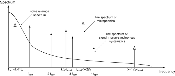
Figure 1: Schematic spectra of signal, noise and systematics for periodic scanning, after demodulation. This spectrum is representative of what is expected for the Planck HFI for one spin-axis position. Possible contribution of microphonics due to periodic vibrations yields, after demodulation, a non-synchronous line spectrum.

Scan synchronous effects, or quasi synchronous noise which cannot be separated from the signal by the filter due to insufficient resolution, cannot be removed from the useful astrophysical signal at this stage. Such signals include those induced by scan-synchronous temperature fluctuations of the payload, and sidelobe effects.

An additionnal use of the analysis on rings is the possibility to compare the spectra of the cosmological signal to that of the noise $\!{}^{{\bf?}}$. This is a precious tool for the optimisation of instrument and mission parameters.

3 Map-making from a set of rings

Assume we now want to reconnect the set of Planck rings into a map. When the main beam of the instrument comes back to a given pixel of the sky, we get a redundant measurement of the same useful astrophysical quantity in a different instrumental configuration. Such redundancies help identifying scan-synchronous effects reprojected on each ring by comparing measurements obtained at crossing points between different rings.

As an illustration of issues related to the identification and subtraction of scan-synchronous effects, we will discuss the problem of sidelobe straylight. The measurement sample $s_{k}$ from the detector at a time $t_{k}$ can be represented, in sampled form, as

$$s_{k} = u_{k}+\sum_{i}L_{i}T_{\rm sky}(p_{k}(i))+n_{k}$$ (3)

$$= u_{k}+M_{kip}L_{i}T_{p}+n_{k}$$ (4)

It has been assumed that the (two-dimensional, band-averaged) sidelobe antenna pattern and the (band-averaged) sky have been pixelised into one dimensional vectors $L_{i}$ and $T_{p}$ repectively. The notation used in equation 3, supposes that for each satellite orientation there is an unambiguous correspondance between sky pixels and antenna pattern pixels, represented by the map $p_{k}(i)$, but this constraining assumption is not necessary when the notation of equation 4 are used. $u_{k}$ is the useful temperature fluctuation in the main beam, and $n_{k}$ the noise (here assumed to be white noise).

The anisotropies we want to measure do not generate significant sidelobe signals. Only bright features (galactic plane, dipole) contribute significantly. A numerical estimate of the sidelobe contribution shows in particular that the Galaxy may generate significant (above noise levels) sidelobe signals, especially in the highest frequency channels.

The absolute temperature of these bright regions of the sky will be measured extremely precisely by Planck (to a relative accuracy of the order of $10^{-2}$ to $10^{-3}$ at least) because noise and systematic effects of any kind (after first-order correction) will be much lower in amplitude than the corresponding signals (which have amplitudes of a few millikelvin). Therefore, equation 4 can be rewritten as $s_{k}=u_{k}+A_{ki}L_{i}+n_{k}$, where $A_{ki}=M_{kip}T_{p}$ is a $N_{k}\times N_{i}$ known matrix, which depends only on the absolute temperature of the sky and on the scan strategy. A possible method to solve the system for $u_{k}$ and $L_{i}$ simultaneously is an iterative one:
a- We first get an estimate of the CMB anisotropies on the sky by standard methods (for instance averaging measurements), neglecting sidelobe effects (or after first-order sidelobe correction using prior knowledge of the antenna pattern). This yields a first order map $\widehat{\Delta T}(\theta,\phi)$.
b- An estimator $\widehat{u_{k}}$ of $u_{k}$ is computed for each sample $k$ by $\widehat{u_{k}}=\Delta T_{1}(\theta_{k},\phi_{k})$, where $(\theta_{k},\phi_{k})$ defines the direction of pointing of the main beam for sample $k$. Differences $\widehat{\delta_{k}}=s_{k}-\widehat{u_{k}}$ are computed.
c- The system $\widehat{\delta_{k}}=A_{ki}L_{i}$ is solved for an estimator $\widehat{L_{i}}$ of $L_{i}$. If the noise is white, the solution is simply $L_{i}=[A^{T}A]^{-1}\,A^{T}\widehat{\delta_{k}}$.
d- The process is iterated with a new estimate of $\delta_{k}$ obtained by correcting for the estimated sidelobe effects using the estimator of $L_{i}$.
There are two important conditions for this prescription to work in practice. The first is that the size of the system be small enough that several iterations can be effectively computed. The second is that matrix $[A^{T}A]$ be regular. The fulfillment of the first condition is insured by the low spatial frequency character of the sources of sidelobe signal, which have significant angular sizes of at least one degree, but usually much more (galactic emission, CMB dipole). Using a model of the sky obtained from extrapolations of the DIRBE data and the DMR dipole templates in the Planck Surveyor wavebands, and several models of Planck Surveyor sidelobes obtained by numerical simulations, we have shown that there is no significant difference between convolution signals calculated using half a degree and three degree resolution maps. It is therefore not necessary, for sidelobe correction, to pixelise the lobe with pixels smaller than a few degrees. The size of vector $L_{i}$ is then a few thousand entries only. The fulfillment of the second condition has been checked with the use of numerical simulations. For the Planck scan strategy, using as a sky template the galactic emission as measured by DIRBE, we have shown that matrix $[A^{T}A]$ is indeed regular, which means that the galactic plane can be used as a source to map the sidelobes. This is very useful in particular for the highest frequency channels of Planck  where the sidelobe contamination from galactic dust is the largest.

4 Conclusion

We have shown that the scan strategy of Planck Surveyor along rings on the sky allows to decompose the problem of converting data streams into CMB anisotropy maps in two independent steps. This makes the problem tractable numerically, and helps in analysing and monitoring the impact of systematic effects. In particular, a promising method for the identification and removal of sidelobe signals has been developped.

References

References

- [1] M. Janssen and S. Gulkis in The infrared and submillimeter sky after COBE; Proceedings of the NATO ASI, Les Houches, France, Mar 20-30, 1991 (A93-51701 22-90)
- [2] J. Delabrouille, K. Górski and E. Hivon, MNRAS in press, astro-ph/9710349 (1997)