The ESO Nearby Abell Cluster Survey

Abstract

We have analyzed the projected galaxy distributions in a subset of the ENACS cluster sample, viz. in those 77 clusters that have z $<$ 0.1 and R${}_{\rm ACO}\geq$ 1 and for which ENACS and COSMOS data are available. For 20 % of these, the distribution of galaxies in the COSMOS catalogue does not allow a reliable centre position to be determined. For the other 62 clusters, we first determined the centre and elongation of the galaxy distribution. Subsequently, we made Maximum-Likelihood fits to the distribution of COSMOS galaxies for 4 theoretical profiles, two with ‘cores’ (generalized King- and Hubble-profiles) and two with ‘cusps’ (generalized Navarro, Frenk and White, or NFW, and de Vaucouleurs profiles).

We obtain average core radii (or characteristic radii for the profiles without core) of 128, 189, 292 and 1582 kpc for fits with King, Hubble, NFW and de Vaucouleurs profiles respectively, with dispersions around these average values of 88, 116, 191 and 771 kpc. The surface density of background galaxies is about 4 10^-5 gals arcsec^-2 (with a spread of about 2 10^-5), and there is very good agreement between the values found for the 4 profiles. There is also very good agreement on the outer logarithmic slope of the projected galaxy distribution, which is that for the non-generalized King- and Hubble-profile (i.e. $\beta_{King}$ = $\beta_{Hubble}$ = 1, with the corresponding values for the two other model-profiles).

We use the Likelihood ratio to investigate whether the observations are significantly better described by profiles with cusps or by profiles with cores. Taking the King and NFW profiles as ‘model’ of either class, we find that about 75 % of the clusters are better fit by the King profile than by the NFW profile. However, for the individual clusters the preference for the King profile is rarely significant at a confidence level of more than 90 %. When we limit ourselves to the central regions it appears that the signifance increases drastically, with 65 % of the clusters showing a strong preference for a King over an NFW profile. At the same time, about 10 % of the clusters are clearly better fitted by an NFW profile than by a King profile in their centres.

We constructed composite clusters from the COSMOS and ENACS data, taking special care to avoid the creation of artificial cusps (due to ellipticity), and the destruction of real cusps (due to non-perfect centering). When adding the galaxy distributions to produce a composite cluster, we either applied no scaling of the projected distances, scaling with the core radii of the individual clusters or scaling with r₂₀₀, which is designed to take differences in mass into account. In all three cases we find that the King profile is clearly preferred (at more than 95 % confidence) over the NFW profile (over the entire aperture of 5 core-radii). However, this ‘preference’ is not shared by the brightest (M${}_{b_{j}}$ $\la$ -18.4) galaxies. We conclude that the brighter galaxies are represented almost equally well by King and NFW profiles, but that the distribution of the fainter galaxies clearly shows a core rather than a cusp.

Finally, we compared the outer slope of the galaxy distributions in our clusters with results for model calculations for various choices of fluctuation spectrum and cosmological parameters. We conclude that the observed profile slope indicates a low value for $\Omega_{0}$. This is consistent with the direct estimate of $\Omega_{0}$ based on the $\frac{M}{L}$-ratios of the individual clusters.

1 Introduction

Until fairly recently, the projected galaxy density in rich galaxy clusters was generally described by King or Hubble profiles. In these profiles, the logarithmic slope of the mass distribution is essentially zero near the cluster centre. The core radius which is the characteristic scale of the distribution, was sometimes also regarded as the distance which more or less separates dynamically distinct regions in a cluster. From the kinematics of the galaxy population it appears that in clusters the relaxation time is significantly shorter than the Hubble time only in the very central region within at most a few core radii (see e.g. den Hartog and Katgert 1996).

The concept of cores in clusters has been seriously challenged, on observational grounds (e.g. Beers $\&$ Tonry 1986) and as a result of numerical simulations. Navarro, Frenk and White (1995, 1996) found e.g. that the equilibrium density profiles of dark matter halos in universes with dominant hierarchical clustering all have the same shape, which is essentially independent of the mass of the halo, the spectrum of initial density fluctuations, or the values of the cosmological parameters. This ‘universal’ density profile (NFW profile hereafter) does not have a core, but has a logarithmic slope of –1 near the centre which, at large radii, steepens to –3, and thus closely resembles the Hernquist (1990) profile except for the steeper slope of the latter at large radii of –4.

Navarro, Frenk and White (1997) argue that the apparent variations in profile shape, as reported before, can be understood as being due to differences in the characteristic density (or mass) of the halo, which sets the linear scale at which the transition of the flat central slope to the steep outer slope occurs. They also argued that the existence of giant arcs in clusters requires that the mass distributions in clusters does not exhibit a flat core in the centre. In other words: if clusters have cores, the lensing results require that the core radii are very small, at least quite a bit smaller than the values usually quoted.

It is not clear that galaxy clusters should have cores; after all, the dynamical structure of galaxy clusters is quite different from that of globular clusters, for which Michie & Bodenheimer (1963) and King first proposed density profiles with cores, in particular the King profile (see e.g. King 1962). On the other hand, the X-ray data for clusters are quite consistent with the existence of a core in the density distribution. More specifically, it was argued recently by Hughes (1997) that the NFW profile would induce a temperature gradient. The existence of such a gradient in the Coma cluster can be excluded at the 99$\%$ confidence level. Similarly, the galaxy surface density in clusters is generally found to be consistent with a King profile. For galaxy clusters, little use has been made of the de Vaucouleurs profile to describe the galaxy density, even though the latter was found to arise quite naturally in N-body simulations of the collapse of isolated galaxy systems (e.g. van Albada 1982).

In view of the claimed universality of the NFW profile found in the simulations, it seems useful to have a closer look at the projected distribution of the galaxies in clusters. After all, the NFW profile refers to the total gravitating mass, and it is not obvious that the galaxy distribution should have exactly the same shape as the distribution of total mass; although in numerical experiments no strong biasing between dark and luminous matter in clusters was seen (e.g. van Kampen 1995). In this respect, it is noteworthy that Carlberg et al. (1997) find that the combined galaxy density profile of 16 high-luminosity X-ray clusters at a redshift of $\approx$0.3 closely follows the NFW profile. More precisely, the logarithmic slope in the central region is consistent with the value of –1 of the NFW and Hernquist profiles, while the outer slope is consistent with both –3 (the NFW value) and –4 (the Hernquist value).

The outer slope of the density profile was found by several authors (e.g. Crone et al. 1994, Jing et al. 1995, and Walter and Klypin 1996) to reflect the details of the formation scenario, and in particular the value of the density parameter of the universe. In addition, this slope is unlikely to be constant in time but is expected to get steeper with decreasing redshift. For that reason, it is important to study both the characteristics of the density profiles of rich clusters and their dependence on redshift.

In this paper, we investigate the projected galaxy distributions for a sample of 62 rich and nearby (z $\la$ 0.1) clusters. These clusters are taken from the volume-limited ENACS (ESO Nearby Abell Cluster Survey) sample of R${}_{\rm ACO}\geq 1$ clusters (see e.g. Katgert et al. 1996 (paper I), Mazure et al. 1996 (paper II), Biviano et al. 1997 (paper III), Adami et al. 1998 (paper IV), Katgert et al. 1998 (paper V) and de Theije $\&$ Katgert 1998 (paper VI)). In $\S$ 2, we first describe the sample of clusters that we used, and the data on which we based our analysis. In $\S$ 3, we discuss the results of Maximum-Likelihood fitting of profiles with and without a core, to the individual galaxy distributions taken from the COSMOS catalogue. In $\S$ 4 we discuss the galaxy density distribution for composite clusters (COSMOS and ENACS), in which the individual clusters are combined. In $\S$ 5 we discuss the constraints provided by the outer slope of the density distributions for the parameters of the formation scenario and in $\S$ 6 we present the conclusions.

2 The data

2.1 The galaxy catalogues

In this paper we use both COSMOS and ENACS data. The COSMOS data, i.e. photometric galaxy catalogues that were obtained from automatic scanning of UK Schmidt IIIa–J survey plates with the Edinburgh plate-scanning machine, were kindly provided by Dr. H.T. MacGillivray. As described in paper V, the COSMOS data that we used are of two kinds: the well-calibrated part around the Southern Galactic Pole (the so-called EDSGC, see e.g. Heydon-Dumbleton et al. 1989), and the slightly less well-calibrated remainder. In paper V, we compared the COSMOS and ENACS photometry and found only a small difference in the calibration quality of the two COSMOS subsets. We did not find evidence for systematic magnitude offsets between the two COSMOS subsets, nor for differences in completeness. From a comparison with the ENACS galaxy catalogues, which are based on completely independent scanning with the Leiden Observatory plate-measuring machine, we concluded that the COSMOS catalogue is 90% complete to a nominal limit of m${}_{b_{j}}$ $\approx$ 19.5.

The galaxy catalogues that resulted from the ENACS spectroscopic survey are described in papers I and V. Very briefly, redshifts were obtained for 5634 galaxies in 107 ACO cluster candidates, mostly in the southern hemisphere. As shown in paper II, the ENACS allowed us to construct a complete, volume-limited sample of 128 rich (R${}_{\rm ACO}\geq$ 1) clusters, out to a redshift of 0.1, when we combine ENACS data for about 80 clusters with literature data for about 50 clusters. In paper V, we have shown the magnitude distributions of the galaxy samples for which we obtained ENACS spectroscopy. Comparison with the magnitude distributions of the COSMOS galaxies shows the ENACS samples to be more or less complete to m${}_{b_{j}}$ between about 18 and 19, with quite a few redshifts for fainter galaxies, viz. down to m${}_{b_{j}}\approx$ 19.5.

2.2 The cluster sample

The overlap of the ENACS dataset with that part of the COSMOS dataset that was available to us yields a sample of 77 clusters. These clusters were not selected according to particular criteria, and we therefore expect them to be a representative subset of the total ENACS sample. To this sample, we have added the cluster A2721, for which we use redshift data from Colless $\&$ Hewett (1987), Colless (1989) and Teague et al. (1990).

Because we want to study density profiles, we are reluctant to use clusters with clear signs of substructure, as for the latter a scale length and the inner and outer slopes of the density profile do not have well-defined meanings. In addition, it is not at all trivial to define a meaningful centre for systems that appear irregular in projection.

In order to give a visual overview of the galaxy distributions in the 77 clusters in the sample, we have used the COSMOS data to produce adaptive-kernel maps for all 77 clusters; these are shown in Figs. 1 and 2.

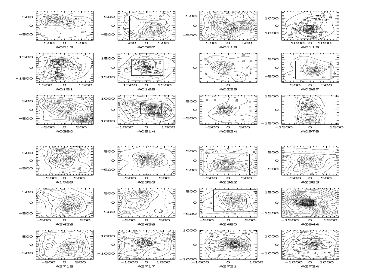
Figure 1: Adaptive-kernel maps of projected galaxy density from the COSMOS catalogue. Coordinates are in arcsec with respect to the cluster centre. Different groups of redshift are indicated as follows: nearest group on the line of sight: circles, 2nd group: squares, 3rd: triangles, 4th: crosses, 5th: asterisks and 6th: stars. We have indicated the area we use for the 29 clusters involved in the COSMOS composite clusters. For A1069, we use the whole area.

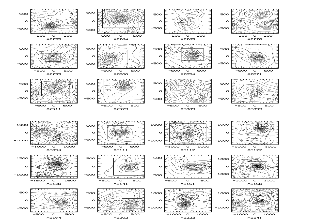
Figure 1: continued

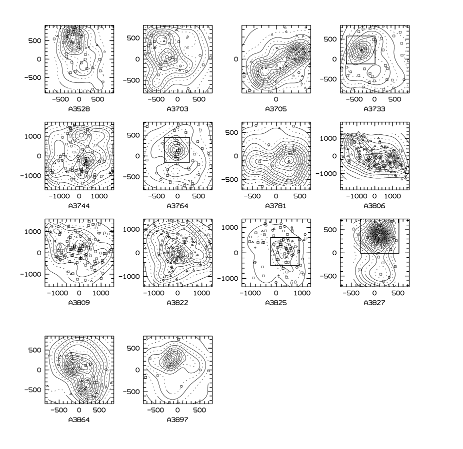
Figure 1: continued

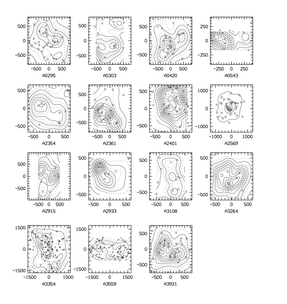
Figure 2: Adaptive-kernel maps of projected galaxy density from the COSMOS catalogue for the 15 clusters for which the centre could not be determined reliably. Coordinates are in arcsec with respect to the cluster centre. The different groups of redshift are characterized by a different symbol: nearest group on the line of sight: circles, 2nd group: squares, 3rd: triangles, 4th: crosses, 5th: asterisks and 6th: stars.

The contour maps in these figures are based on surface densities calculated as the sum of normalized gaussian kernel functions at the positions of the galaxies with dispersions $\sigma_{i}$ that are adapted to the local galaxy density (e.g. Silverman 1986). In Figs. 1 and 2 , it is fairly easy to distinguish clusters with single density peaks, clusters with multiple density peaks that can be clearly separated and/or identified with systems at different redshifts, and irregular clusters. By using different symbols for systems with different redshifts (see papers I and IV), it is possible to recognize clusters which consist of several ‘single’ peaks at different redshifts. About two-thirds of the clusters in our sample show a single peak, while about 10% was considered irregular. We have defined the studied area for each cluster as the maximal area without a clear sign of substructure and with a single density peak. Afterwards, we have checked that these areas comprise more than 5 King core radii (i.e. with a radius greater than 500 kpc).

In Tab. 1, we give our verdict on the character of the galaxy distribution, as well as some other information, for the 62 clusters in Fig. 1 for which a central position could be determined reliably (see $\S$ 3). The 15 clusters for which no reliable position could be obtained are shown in Fig. 2; those could not be used in the following analysis. It should be noted that Tab. 1 has 2 entries for A0151, while the cluster A3559 (in the region of the Shapley concentration) was discarded because it did not show a clear maximum in the galaxy distribution. Note also that our verdict ‘regular’ in Tab. 1 does not imply that the cluster does not have substructure, as projection may hide substructure along the line-of-sight.

The mean redshift of the systems in Tab. 1 is about 0.075 (practically equal to that of the total ENACS sample). In the following analysis we will adopt $H_{0}$ = 100 km/s/Mpc and $q_{0}$ = 0. The parameters will be determined with robust statistical estimators (Beers et al. 1990).

Table 1: Parameters of the 62 clusters for which a reliable centre position was obtained. Col.(1) cluster name, col.(2) ENACS redshift of the group, col (3) type of galaxy distribution (0: regular single peak, 1: multimodal, 2: irregular), cols.(4) and (5) centre position, col (6) ellipticity (when available) and col (7) direction of the major axis (if ellipticity available and not equal to 0), counted anti-clockwise from $\delta$=0.

ACO	z	type	$\alpha$	$\delta$	e	$\phi$
			2000.0
0013	0.094	0	00:13:34.53	-19:29:38	0.32	-16
0087	0.055	0	00:43:00.73	-09:50:37	0.00
0118	0.115	1	00:55:21.47	-26:23:24	0.00
0119	0.044	0	00:56:20.13	-01:15:51	0.00
0151	0.041	0	01:08:50.07	-15:25:05	0.14	-25
0151	0.053	2	01:08:52.73	-15:56:51	0.00
0168	0.045	0	01:15:14.87	00:15:23	0.00
0229	0.113	0	00:14:34.47	00:01:21	0.50	-45
0367	0.091	0	02:36:35.20	-19:22:16	0.05	70
0380	0.134	1	02:44:23.33	-26:13:58	0.12	-43
0514	0.072	1	04:48:15.13	-20:27:26	0.28	-25
0524	0.078	0	04:57:47.87	-19:43:11
0978	0.054	1	10:20:24.33	-06:29:53	0.04	0
1069	0.065	0	10:39:47.93	-08:40:46	0.00
2353	0.121	0	21:34:27.33	-01:36:15
2362	0.061	0	21:39:03.33	-14:21:10	0.23	-2
2383	0.058	0	21:52:10.00	-21:09:35
2426	0.098	0	22:14:35.33	-10:21:51	0.00
2436	0.091	2	22:20:31.33	-02:46:57	0.21	28
2480	0.072	0	22:46:10.67	-17:41:22	0.08	-52
2644	0.069	0	23:41:02.00	00:05:30	0.29	-20
2715	0.114	0	00:02:48.60	-34:40:57	0.00
2717	0.049	2	00:03:07.73	-35:56:50	0.00
2721	0.120	0	00:06:12.53	-34:43:12	0.00
2734	0.062	0	00:11:22.93	-28:50:55	0.00
2755	0.095	0	00:17:39.20	-35:11:57	0.07	27
2764	0.071	0	00:20:29.53	-49:14:14	0.00
2765	0.080	0	00:21:31.53	-20:45:55	0.00
2778	0.102	1	00:29:08.67	-30:17:28	0.00
2799	0.063	0	00:37:24.13	-39:09:01	0.17	5
2800	0.064	0	00:37:58.67	-25:05:17	0.37	35
2854	0.061	0	01:00:47.20	-50:32:38	0.54	-68
2871	0.122	0	01:08:08.07	-36:45:30	0.00
2911	0.064	0	01:26:08.00	-37:57:26	0.00
2923	0.061	0	01:32:28.80	-31:04:41	0.00
3009	0.120	2	02:21:33.53	-48:28:43
3093	0.081	0	03:10:54.93	-47:23:53
3094	0.071	1	03:12:36.67	-27:08:05	0.00
3094	0.065	1	03:11:23.13	-26:54:21	0.00
3111	0.083	0	03:17:49.00	-45:43:38	0.02	30
3112	0.075	0	03:17:58.53	-44:14:21	0.30	73
3122	0.068	0	03:22:14.00	-41:19:14	0.00
3128	0.078	1	03:30:37.87	-52:31:51	0.00
3141	0.075	0	03:36:54.27	-28:04:20	0.44	50
3151	0.064	0	03:40:07.80	-28:41:27
3158	0.060	0	03:43:04.60	-53:38:40	0.00
3194	0.105	0	03:59:07.20	-30:11:24
3202	0.059	0	04:00:55.53	-53:41:17	0.13	49
3223	0.060	1	04:08:05.80	-31:03:20	0.27	61
3341	0.038	2	05:25:34.20	-31:36:35	0.06	41
3528	0.054	0	12:54:24.07	-29:02:05
3703	0.074	2	20:39:52.67	-61:19:34
3705	0.090	2	20:42:04.00	-35:13:07	0.65	35
3733	0.039	0	21:01:34.67	-28:02:42	0.49	35
3744	0.038	1	21:07:26.00	-25:24:36	0.00
3744	0.038	1	21:07:09.33	-25:01:56
3764	0.075	0	21:25:47.33	-34:42:44	0.35	-28
3781	0.057	0	21:35:27.33	-66:49:14
3806	0.076	2	21:46:24.00	-57:17:28	0.22	-15
3806	0.076	2	21:48:09.33	-57:17:15
3809	0.062	2	21:47:17.33	-43:52:54	0.00
3822	0.076	1	21:54:03.33	-57:50:27	0.00
3825	0.075	0	21:58:26.00	-60:22:03	0.00
3827	0.098	0	22:01:52.00	-59:56:42	0.00
3864	0.102	1	22:19:47.33	-52:27:05	0.00
3897	0.073	0	22:39:10.67	-17:20:14	0.00

3 The density profiles of the individual clusters

3.1 The Maximum-Likelihood fits

We derived the characteristics of the projected galaxy distributions for the individual clusters using Maximum-Likelihood fits (hereafter MLM fits, see e.g. Sarazin 1980 for a description of the method). We have made MLM fits for different types of profile as follows. Define $\sigma(x,y)$ as the theoretical, normalized density profile with which one wants to compare the data. Note that we scaled the amplitude of the model to reproduce the observed number of galaxies.

The probability that this assumed profile ‘produces’ a galaxy in position (x_k,y_k) is thus $\sigma(x_{k},y_{k})$. Consequently, the combined probability that the assumed profile will ‘produce’ galaxies in the positions (x_k,y_k) (with k=1…N) that they actually have is:

L=$\prod\limits_{k=1}^{N}\sigma(x_{k},y_{k})$

The model-parameters which produce the best fit between the data and the model are found from a maximization of the likelihood L. The combined probability, L, for all galaxies to have their actual positions assuming the model to be correct, is always less than unity. For that reason, in practice, one usually minimizes the positive parameter –2ln(L) w.r.t. the parameters of the assumed profile. This yields the values of the parameters for which the model is most likely to have generated the N galaxies at their observed positions. The great advantage of this method is that it does not require the data to be binned. In addition, it uses all information that is available.

The minimization of –2ln(L) was done with the two minimization methods in the MINUIT package: SIMPLEX (Nelder $\&$ Mead, 1965) and MIGRAD (Fletcher 1970). We use the same stategy as described in paper IV to obtain convergence. Viz., we use SIMPLEX to approach the optimal values and MIGRAD to refine those and get reliable error estimates. When MIGRAD did not converge, we adopted the SIMPLEX value without error estimates.

We used the following model profiles for the 2D galaxy distributions:

- generalized King model: $\sigma(r)=\sigma_{0}(\frac{1}{1+(\frac{r}{r_{c}})^{2}})^{\beta}+\sigma_{b}$,

- generalized Hubble model: $\sigma(r)=\sigma_{0}(\frac{1}{1+\frac{r}{r_{c}}})^{2\beta}+\sigma_{b}$,

- generalized NFW model: $\sigma(r)=\sigma_{0}(\frac{1}{\frac{r}{r_{c}}(1+\frac{r}{r_{c}})^{2}})^{\beta}+\sigma_{b}$,

Note that the 2-D model profile that we refer to as NFW is not an exact 2-D version of the 3-D profile described by NFW. Instead, it is a pseudo NFW profile, with a relation between 3-D and 2-D outer logartithmic slopes as for the King and Hubble profiles, but with an inner logarithmic slope equal to that of the 3-D NFW profile.

- generalized de Vaucouleurs model: $\sigma(r)=\sigma_{0}e^{-\beta(\frac{r}{r_{c}})^{0.25}}+\sigma_{b}$.

As the actual clusters are not necessarily axi-symmetric, the models have 7 free parameters: two parameters for the position of the centre (x₀, y₀), two parameters to describe deviations from symmetry (ellipticity e and position angle $\phi$), two parameters that specify the profile (r_c and $\beta$) and, finally, the background density $\sigma_{b}$ (assumed constant within the aperture of each cluster).

In principle, an MLM solution could have been made for all 7 parameters simultaneously. However, we have separated the solution for the central position and the elongation and position angle, from the solution of the background density and the profile parameters r_c and $\beta$. More precisely: we used a King profile with r_c = 100 kpc, $\beta$ = 1.0, and we assumed a value for $\sigma_{b}$ of 3 10^-5 galaxies per square arcsec to make an MLM fit for x₀, y₀, e, and $\phi$. As mentioned previously, this fit did not converge for 15 clusters, viz. for A0295, A0303, A0420, A0543, A2354, A2361, A2401, A2569, A2915, A2933, A3108, A3264, A3354, A3559 and A3921. These clusters could therefore not be used for MLM fits for the four profiles.

The average uncertainty in the central position as given by the fits is about 30 kpc. This is not too different from, but somewhat smaller than the measured offsets between fitted positions and literature X-ray centres or literature positions of cD galaxies as given in Tab. 2. Except for the clusters A0514, A3009 and A3128, which are either double-peaked or irregular, and apart from A3825 all offsets are smaller than 100 kpc, and the biweight average measured offset between fitted positions and X-ray or cD positions is 51 kpc.

Table 2: Literature positions for 17 clusters with either X-ray or cD centre position. Col.(1) cluster name, cols.(2) and (3) literature centre, col.(4) distance between literature and fitted centre in kpc, col.(5) type of literature centre (X or cD)

ACO	$\alpha$	$\delta$	dist.	type
	2000.0		(kpc)
0119	00:56:17.80	-01:15:23	27	X
0151	01:08:50.59	-15:24:26	22	cD
0168	01:15:08.44	00:17:11	88	X
0514	04:48:30.35	-20:32:09	413	X
1069	10:39:44.29	-08:41:25	58	X
2426	22:14:31.45	-10:22:27	87	X
2734	00:11:21.56	-28:51:15	22	cD
2911	01:26:05.51	-37:57:54	35	cD
2923	01:32:21.40	-31:05:31	88	cD
3009	02:22:06.88	-48:33:49	664	cD
3112	03:17:56.95	-44:13:59	47	X
3128	03:30:50.85	-52:30:31	485	X
3158	03:42:56.64	-53:38:04	63	X
3528	12:54:23.54	-29:01:24	34	X
3806	21:46:21.77	-57:17:11	19	cD
3825	21:58:40.28	-60:19:57	162	X
3827	22:01:57.88	-59:56:18	52	X

In Tab. 3 and Fig. 3, we show a comparison with the more homogeneous ROSAT sample of X-ray centres (preliminary centres kindly provided by H. Bohringer). The biweight average offset between fitted positions and X-ray centres is 78 kpc. If we ignore the clusters with an atypical offset of more than 150 kpc, we obtain 69 kpc. The clusters that we considered atypical are A0380 which is a clear double-peaked cluster, A3809 which is irregular, A2871 which exhibits clearly a very atypical difference of 449 kpc, A0524 and A2799. We have checked the internal accuracy of the ROSAT centres by using the X-ray map of A0119 (kindly provided by D. Neumann). We estimate that this error is about 20” (11 kpc) for A0119. However, we deal we a very regular cluster and the error is probably underestimated compared to the other clusters. Another way to estimate the global error of the ROSAT centres is to compare with other literature positions (X-ray or cD). We find a mean offset of 31 kpc (see Tab. 3), greater than the 11 kpc obtained for A0119.

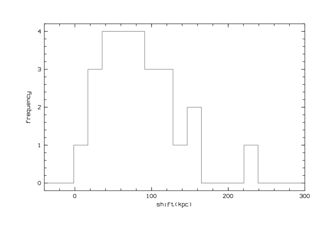
Figure 3: The histogram of the offsets between the X-Ray ROSAT and the fitted centres. The two clearly atypic values for A0380 and A2871 are not shown.

Table 3: ROSAT X-ray centre positions for 28 clusters. Col.(1) cluster name, cols.(2) and (3) ROSAT centre, col.(4) distance between ROSAT and fitted centre in kpc, col.(5) distance between ROSAT and previous literature centre in kpc (when available).

ACO	$\alpha$	$\delta$	dist.	dist. ROSAT/Lit
	2000.0		(kpc)	(kpc)
0013	00:13:38.23	-19:30:08	75
0119	00:56:14.60	-01:15:44	47	40
0151	01:08:50.47	-15:24:33	18	4
0367	02:36:39.34	-19:23:09	94
0380	02:44:05.69	-26:11:17	501
0524	04:57:57.19	-19:43:58	150
0978	10:20:28.72	-06:31:14	75
1069	10:39:44.81	-08:41:01	42	22
2426	22:14:32.38	-10:22:12	61	25
2717	00:03:11.14	-35:55:21	74
2734	00:11:20.28	-28:51:31	44	21
2755	00:17:34.90	-35:11:09	97
2764	00:20:34.10	-49:13:40	72
2799	00:37:29.47	-39:06:18	152
2871	01:07:49.37	-36:43:44	449
2911	01:26:04.56	-37:58:36	71	38
3093	03:10:55.15	-47:24:31	40
3112	03:17:58.27	-44:14:16	7	25
3122	03:22:18.19	-41:21:29	136
3158	03:42:54.82	-53:38:08	120	22
3194	03:59:08.16	-30:11:36	25
3341	05:25:32.66	-31:35:56	24
3744	21:07:13.49	-25:26:54	122
3806	21:46:27.00	-57:16:47	60	81
3809	21:46:57.72	-43:54:33	224
3822	21:54:09.62	-57:51:15	105
3825	21:58:27.26	-60:23:56	113
3827	22:01:55.90	-59:56:57	76

The values of the ellipticities are mostly quite small, and even indistinghuisable from 0.0 for quite a few of the clusters. This might seem to be in contradiction to other results on the elongation of clusters (e.g. Plionis et al. 1991, and de Theije et al. 1995). However, it must be appreciated that our ellipticities are apparent ellipticities, i.e. not corrected for the effect of the aperture, and that they refer to the central regions only (about 5 King core radii: i.e. a radius of slightly more than 500 kpc).

3.2 The values of r_c, $\beta$ and $\sigma_{b}$

Using the fitted values of x₀, y₀, e, and $\phi$ we subsequently made MLM fits for r_c, $\beta$ and $\sigma_{b}$, for the 62 clusters in Tab. 1, for each of the 4 profiles, for which the solution of x₀, y₀, e, and $\phi$ converged.

In Tabs. 4 to 7, we give the values of r_c, $\beta$ and $\sigma_{b}$ for all clusters in the sample of 62, i.e. for all clusters with a reliable centre position, for each of the model profiles. For some of the clusters, one or more of the MLM fits did not converge for one or more of the parameters. In those cases we give the SIMPLEX values without error estimates. The error estimates obtained for each of the 3 parameters, as given by MIGRAD are also given in Tabs. 4 to 7, in which we also give the values of –2ln(L). As is well known, the magnitude of this parameter (the maximum likelihood for the particular model profile with the best-fit parameters) cannot be used to make a statement about the absolute probability that a given observation is indeed induced by the underlying continuous probability function described by the particular profile.

As a check on the ‘meaning’ of the error estimates from MIGRAD, we have generated about 150000 artificial clusters, for which the total number of galaxies, the ratio between the number of galaxies in the cluster and in the background, and r_c- and $\beta$-values for the 4 model profiles were chosen in the ranges spanned by the observations. To each of the artificial clusters a MLM fit was made in the same manner as for the observed clusters. The errors in the parameters of the fits to the artifical clusters depend somewhat on the type of profile and on the assumed parameters, but globally, the results can be summarized as follows.

The background density is recovered with an average accuracy of about 25% (with actual errors between about 10 and 40%), with a slightly better result for the King and Hubble profiles than for the NFW and de Vaucouleurs profiles (which is not surprising). Almost identical percentage errors are found for r_c. In general, $\beta$ is slightly better known, with an average error of about 15% (with actual errors between about 5 and 25%). As can be seen from Tabs. 4 to 7, the errors given by MIGRAD are essentially always in the ranges found for the artificial clusters.

Table 4: Fitted parameters for the King models and contrast (last column).

ACO	$r_{c}$ (kpc)	$\beta$	$\sigma_{b}$	–2ln(L)	C
0013	68$\pm$18	0.97$\pm$0.11	8.7$\pm$1.0	2397.90	0.504
0087	118$\pm$12	1.06$\pm$0.15	3.0$\pm$0.6	1624.15	0.346
0118	118$\pm$44	1.04$\pm$0.07	9.1$\pm$1.3	1622.29	0.262
0119	55$\pm$14	1.07$\pm$0.10	4.5$\pm$0.2	6963.61	0.510
0151	56$\pm$ 9	1.18$\pm$0.15	4.6$\pm$0.4	3999.36	0.646
0168	161$\pm$42	1.01$\pm$0.28	4.2$\pm$0.9	2179.73	0.454
0229	43	0.97	9.0	839.70	0.784
0367	128$\pm$21	1.23$\pm$0.13	3.4$\pm$0.7	2043.15	0.537
0380	496$\pm$86	1.02$\pm$0.22	2.0$\pm$0.2	1753.21	0.976
0514	90$\pm$25	1.01$\pm$0.14	5.4$\pm$1.1	2358.88	0.547
0524	95$\pm$23	1.04$\pm$0.09	1.1$\pm$0.5	1495.57	0.823
0978	44$\pm$12	0.94$\pm$0.15	3.5$\pm$0.3	3564.50	0.648
1069	219$\pm$65	1.03$\pm$0.29	3.0$\pm$1.0	2704.82	0.465
2353	163$\pm$40	0.96$\pm$0.12	2.9$\pm$1.6	1839.96	0.519
2362	110$\pm$32	1.01$\pm$0.28	4.6$\pm$1.2	1636.26	0.256
2383	86$\pm$19	0.95$\pm$0.12	3.1$\pm$0.6	2304.33	0.517
2426	135$\pm$26	0.84$\pm$0.08	5.7$\pm$0.9	5044.65	0.579
2436	79$\pm$37	1.00$\pm$0.19	7.0$\pm$0.9	1195.09	0.318
2480	101$\pm$28	1.09$\pm$0.33	4.8$\pm$0.9	1434.17	0.309
2644	76$\pm$22	1.00$\pm$0.14	3.3$\pm$0.8	1249.19	0.846
2715	236	1.00	3.0	2639.96	0.594
2717	140$\pm$40	0.99$\pm$0.11	3.2$\pm$0.4	4859.57	0.470
2721	286$\pm$34	0.96$\pm$0.08	3.5$\pm$1.0	6146.76	0.696
2734	105$\pm$22	1.00$\pm$0.11	3.6$\pm$0.4	5277.62	0.567
2755	49$\pm$10	1.01$\pm$0.07	9.5$\pm$0.9	3842.01	0.754
2764	101$\pm$22	1.00$\pm$0.13	5.6$\pm$0.9	3514.23	0.511
2765	66$\pm$22	0.98$\pm$0.19	2.9$\pm$0.4	1757.98	0.661
2778	98$\pm$26	1.01$\pm$0.13	4.1$\pm$0.7	1746.72	0.577
2799	46$\pm$11	0.94$\pm$0.33	4.5$\pm$0.5	2022.80	0.514
2800	99$\pm$25	1.01$\pm$0.14	4.0$\pm$0.6	2050.76	0.282
2854	67$\pm$17	1.01$\pm$0.10	2.6$\pm$0.7	1517.14	0.643
2871	139$\pm$30	1.06$\pm$0.22	2.1$\pm$0.8	2306.66	0.796
2911	109$\pm$28	1.13$\pm$0.30	8.8$\pm$0.9	2842.87	0.268
2923	142$\pm$19	1.33$\pm$0.18	2.1$\pm$0.6	1110.31	0.914
3009	45$\pm$33	0.99$\pm$0.20	7.4$\pm$0.5	1623.65	0.230
3093	69$\pm$21	1.00$\pm$0.12	5.7$\pm$1.6	1544.33	0.457
3094	127$\pm$30	1.01$\pm$0.16	5.7$\pm$0.8	2907.21	0.458
3111	99$\pm$26	1.00$\pm$0.03	4.2$\pm$0.4	5842.78	0.591
3112	229$\pm$29	1.02$\pm$0.28	3.7$\pm$1.8	2277.64	0.502
3122	150$\pm$20	0.97$\pm$0.07	3.2$\pm$0.5	6535.82	0.564
3128	362$\pm$29	1.08$\pm$0.08	3.1$\pm$0.5	12479.20	0.500
3141	176$\pm$32	0.97$\pm$0.10	1.3$\pm$0.7	1646.93	0.870
3158	102$\pm$15	0.95$\pm$0.07	4.5$\pm$0.7	7446.85	0.639
3194	54$\pm$ 7	1.02$\pm$0.23	7.0$\pm$1.3	1306.30	0.601
3202	64$\pm$21	0.99$\pm$0.14	3.6$\pm$1.0	1652.64	0.657
3223	154$\pm$39	1.01$\pm$0.12	3.0$\pm$1.6	2632.48	0.674
3341	51$\pm$12	0.95$\pm$0.13	4.0$\pm$0.8	2239.58	0.466
3528	135$\pm$35	1.06$\pm$0.26	9.0$\pm$3.0	3130.11	0.311
3705	99$\pm$28	0.98$\pm$0.20	6.7$\pm$2.3	999.64	0.639
3733	37$\pm$11	1.07$\pm$0.15	3.1$\pm$0.9	1183.78	0.659
3744	79$\pm$19	1.10$\pm$0.23	4.2$\pm$0.6	2339.98	0.188
3764	59$\pm$16	1.31$\pm$0.18	5.5$\pm$0.7	1754.89	0.556
3781	232$\pm$71	1.01$\pm$0.21	2.6$\pm$1.5	1580.22	0.520
3806	224$\pm$30	1.01$\pm$0.12	1.1$\pm$1.5	2953.74	0.688
3806	106$\pm$33	1.00$\pm$0.23	14.$\pm$13.	3533.92	0.669
3809	365$\pm$58	1.00$\pm$0.23	2.5$\pm$1.2	5251.67	0.708
3822	242$\pm$32	1.04$\pm$0.11	8.4$\pm$1.1	7313.07	0.282
3825	108$\pm$26	0.97$\pm$0.12	8.8$\pm$1.0	3802.11	0.245
3827	102$\pm$17	1.00$\pm$0.09	5.0$\pm$1.6	2646.64	0.707
3897	76	1.01	4.0	1028.79	0.498

Table 5: Fitted parameters for the Hubble models.

ACO	$r_{c}$ (kpc)	$\beta$	$\sigma_{b}$	–2ln(L)
0013	122$\pm$14	0.97$\pm$0.11	5.3$\pm$1.3	2399.12
0087	183$\pm$51	1.02$\pm$0.25	1.5$\pm$0.6	1624.63
0118	135$\pm$33	1.01$\pm$0.25	10.0$\pm$1.4	1623.69
0119	73$\pm$10	1.14$\pm$0.10	4.0$\pm$0.9	6965.28
0151	94$\pm$16	1.19$\pm$0.17	7.5$\pm$1.0	4001.52
0168	178$\pm$28	0.98$\pm$0.14	1.7$\pm$1.9	2182.01
0367	162$\pm$26	1.23$\pm$0.14	2.6$\pm$1.2	2043.29
0380	556$\pm$95	0.98$\pm$0.24	0.6$\pm$2.0	1754.17
0514	117$\pm$33	1.06$\pm$0.15	6.3$\pm$2.1	2359.08
1069	411$\pm$65	1.03$\pm$0.19	1.1$\pm$1.3	2705.29
2353	198$\pm$32	0.93$\pm$0.04	0.8$\pm$1.2	1838.87
2362	257$\pm$28	1.05$\pm$0.13	1.1$\pm$0.7	1636.31
2383	88$\pm$33	0.99$\pm$0.21	2.1$\pm$1.6	2303.26
2426	253$\pm$22	1.01$\pm$0.36	7.0$\pm$0.9	5048.38
2480	272	1.01	3.5	1435.84
2644	118$\pm$33	0.97$\pm$0.35	1.3$\pm$0.5	1251.32
2715	100$\pm$25	0.99$\pm$0.25	5.8$\pm$1.3	2642.28
2717	156$\pm$23	1.00$\pm$0.29	2.7$\pm$0.9	4859.71
2721	264$\pm$42	0.97$\pm$0.46	5.0$\pm$1.5	6148.75
2734	137	0.99$\pm$0.14	3.7	5277.09
2755	54$\pm$ 7	0.99$\pm$0.20	7.1$\pm$1.5	3842.10
2764	126$\pm$25	1.01$\pm$0.12	6.6$\pm$1.9	3514.66
2799	48$\pm$15	1.02$\pm$0.10	5.4$\pm$0.9	2024.67
2800	87$\pm$26	1.01$\pm$0.25	4.6	2052.23
2854	70$\pm$11	1.13$\pm$0.16	2.0$\pm$0.9	1517.04
2871	142$\pm$17	0.99$\pm$0.14	0.9$\pm$0.5	2308.41
2923	96$\pm$19	1.01$\pm$0.11	0.2$\pm$1.8	1114.55
3094	300	1.07	3.4	2908.45
3111	180$\pm$23	1.01$\pm$0.15	0.1$\pm$0.7	5846.81
3112	248$\pm$65	1.01$\pm$0.18	5.0$\pm$0.9	2277.91
3122	319	1.19	1.6	6534.76
3128	520$\pm$39	1.01$\pm$0.25	1.1$\pm$1.2	12480.05
3158	104$\pm$12	0.87$\pm$0.18	4.2$\pm$1.3	7445.38
3202	132$\pm$39	1.18$\pm$0.18	3.7$\pm$1.5	1653.53
3223	211$\pm$24	1.01$\pm$0.20	2.0$\pm$1.0	2632.55
3341	133$\pm$19	1.11$\pm$0.19	1.6$\pm$1.1	2240.54
3733	84$\pm$15	1.01$\pm$0.11	3.1$\pm$1.5	1185.51
3744	155$\pm$22	0.96$\pm$0.20	1.1$\pm$0.5	2340.79
3764	97$\pm$12	1.13$\pm$0.29	6.7$\pm$1.0	1760.46
3781	297$\pm$75	1.02$\pm$0.30	1.1$\pm$0.8	1579.93
3806	200$\pm$38	1.01$\pm$0.19	10.5$\pm$2.2	2959.95
3806	284$\pm$31	1.04$\pm$0.13	3.0$\pm$6.9	3535.88
3822	378$\pm$61	1.06$\pm$0.23	6.6$\pm$0.9	7313.49
3825	244$\pm$50	0.97$\pm$0.10	7.0$\pm$2.0	3803.01
3827	119$\pm$13	1.01$\pm$0.08	4.3$\pm$0.7	2646.25

Table 6: Fitted parameters for the NFW models.

ACO	$r_{c}$ (kpc)	$\beta$	$\sigma_{b}$	–2ln(L)
0013	128$\pm$63	0.64$\pm$0.07	8.4$\pm$1.1	2399.69
0087	324$\pm$35	0.68$\pm$0.13	2.8$\pm$0.7	1625.99
0118	169$\pm$134	0.58$\pm$0.13	10.0$\pm$1.8	1624.48
0119	146$\pm$25	0.70$\pm$0.10	4.0$\pm$0.6	6965.88
0151	112$\pm$28	0.68$\pm$0.14	4.5$\pm$1.1	4000.93
0168	210$\pm$39	0.56$\pm$0.10	1.0$\pm$0.4	2179.72
0367	286$\pm$44	0.62$\pm$0.11	1.4$\pm$0.9	2043.92
0524	141$\pm$55	0.62$\pm$0.05	0.2$\pm$0.6	1497.56
0978	94$\pm$50	0.64$\pm$0.07	3.3$\pm$0.3	3564.57
1069	281$\pm$34	0.61$\pm$0.09	4.9$\pm$1.1	2707.30
2353	327$\pm$175	0.59$\pm$0.07	2.6$\pm$1.0	1838.57
2362	248$\pm$49	0.55$\pm$0.10	3.0$\pm$1.0	1636.39
2383	143$\pm$86	0.66$\pm$0.08	3.3$\pm$0.6	2301.49
2426	458$\pm$185	0.63$\pm$0.07	5.0$\pm$1.1	5044.38
2436	193$\pm$192	0.66$\pm$0.17	7.0$\pm$1.2	1195.58
2480	430$\pm$50	0.60$\pm$0.09	4.0$\pm$0.8	1436.00
2644	106$\pm$37	0.55$\pm$0.06	2.5$\pm$0.4	1251.34
2717	458$\pm$238	0.58$\pm$0.06	1.8$\pm$0.6	4859.71
2721	649	0.55	2.0	6150.09
2734	253$\pm$35	0.53$\pm$0.11	3.0$\pm$1.2	5276.62
2755	173$\pm$63	0.67$\pm$0.07	5.9$\pm$1.1	3841.34
2764	356$\pm$46	0.61$\pm$0.09	5.5$\pm$0.6	3515.77
2765	147$\pm$96	0.55$\pm$0.08	2.0$\pm$0.6	1757.89
2778	390$\pm$239	0.70$\pm$0.09	2.8$\pm$1.0	1746.35
2799	296$\pm$52	0.67$\pm$0.12	2.7$\pm$0.6	2022.63
2800	266$\pm$43	0.59$\pm$0.09	2.7$\pm$1.0	2052.00
2854	150$\pm$35	0.69$\pm$0.07	2.1$\pm$0.7	1516.08
2871	226$\pm$75	0.57$\pm$0.05	0.5$\pm$1.0	2310.69
2911	392$\pm$48	0.59$\pm$0.05	6.3$\pm$0.3	2844.33
2923	123$\pm$43	0.63$\pm$0.06	0.2$\pm$0.6	1115.98
3009	95	0.61	7.4	1623.92
3093	362	0.62	3.0	1543.66
3094	247$\pm$121	0.57$\pm$0.09	6.0$\pm$1.0	2909.27
3111	144$\pm$66	0.51$\pm$0.04	4.1$\pm$0.5	5848.95
3112	455$\pm$57	0.57$\pm$0.10	6.6$\pm$1.7	2279.49
3122	339	0.53	7.1	6535.54
3128	966	0.59	2.7	12484.70
3158	430$\pm$151	0.63$\pm$0.07	3.3$\pm$1.1	7442.27
3194	100$\pm$54	0.65$\pm$0.09	6.5$\pm$1.6	1308.37
3202	348$\pm$41	0.69$\pm$0.06	4.8$\pm$0.8	1652.14
3341	275$\pm$190	0.61$\pm$0.04	3.0$\pm$1.0	2240.44
3528	168	0.57	2.3	3143.42
3705	340$\pm$205	0.66$\pm$0.08	3.8$\pm$3.3	995.70
3733	99$\pm$29	0.64$\pm$0.09	3.8$\pm$1.0	1185.51
3744	202$\pm$133	0.67$\pm$0.12	3.9$\pm$0.7	2342.55
3764	100$\pm$39	0.68$\pm$0.07	5.4$\pm$1.0	1757.60
3781	849$\pm$598	0.69$\pm$0.15	3.5$\pm$1.1	1578.26
3806	671$\pm$492	0.55$\pm$0.11	10.0$\pm$2.6	3534.19
3809	541$\pm$334	0.54$\pm$0.09	5.2$\pm$0.9	5254.24
3827	181$\pm$81	0.61$\pm$0.05	4.4$\pm$2.4	2647.14

Table 7: Fitted parameters for the de Vaucouleurs models.

ACO	$r_{c}$ (kpc)	$\beta$	$\sigma_{b}$	–2ln(L)
0013	1441$\pm$379	7.46$\pm$0.87	5.4$\pm$1.4	2399.25
0087	691	7.32	3.3	1626.20
0118	2961$\pm$1778	7.42$\pm$1.59	6.5$\pm$2.5	1623.77
0119	861$\pm$210	7.60$\pm$0.76	3.8$\pm$0.3	6969.06
0151	573$\pm$260	7.78$\pm$0.94	3.8$\pm$ 0.5	4001.32
0168	1031$\pm$104	7.45$\pm$0.60	5.0$\pm$0.7	2179.82
0367	1535$\pm$580	7.70$\pm$0.83	1.4$\pm$0.8	2043.87
0380	4762	7.03	2.6	1755.37
0514	1752$\pm$304	7.60$\pm$0.78	6.4$\pm$1.5	2359.24
0524	1146$\pm$403	8.92$\pm$0.74	0.9$\pm$0.5	1497.69
0978	458$\pm$200	7.82$\pm$0.86	3.4$\pm$0.3	3564.55
1069	1365$\pm$411	7.51$\pm$0.89	4.5$\pm$0.9	2708.09
2353	1197$\pm$582	7.06$\pm$0.90	3.0$\pm$0.9	1837.85
2362	1721$\pm$304	8.05$\pm$0.92	4.1$\pm$0.3	1636.56
2383	1184$\pm$576	7.95$\pm$0.96	2.7$\pm$0.7	2301.50
2426	1272	7.50	6.4	5045.18
2436	1438$\pm$1060	8.72$\pm$2.17	7.0$\pm$1.3	1195.54
2480	1161$\pm$286	7.52$\pm$0.58	4.6$\pm$1.1	1436.05
2644	1074$\pm$311	7.78$\pm$0.79	2.5$\pm$0.8	1251.41
2717	1971$\pm$841	6.59$\pm$0.72	2.0$\pm$0.7	4859.83
2721	2879$\pm$1043	6.42$\pm$0.51	2.3$\pm$1.3	6149.83
2734	1932$\pm$298	7.89$\pm$0.70	3.6$\pm$0.5	5277.25
2755	2077$\pm$655	9.24$\pm$0.69	4.0$\pm$1.3	3842.03
2764	3165$\pm$379	7.87$\pm$0.55	5.0$\pm$1.3	3515.44
2765	1460$\pm$840	7.62$\pm$1.11	2.0$\pm$0.6	1757.91
2778	1263	7.51	2.8	1746.40
2799	787$\pm$255	7.56$\pm$0.33	3.3$\pm$0.8	2022.67
2800	1712$\pm$213	7.80$\pm$0.83	3.1$\pm$0.8	2051.98
2854	802$\pm$266	7.82$\pm$0.72	1.7$\pm$0.7	1516.30
2871	1608	7.84	0.4	2310.71
2911	2213$\pm$266	7.18$\pm$0.22	6.4$\pm$1.4	2844.38
2923	735$\pm$207	8.12$\pm$0.57	3.0$\pm$0.3	1116.00
3009	2302	7.61	6.9	1623.90
3093	1028	6.99	3.6	1543.57
3094	1406	7.52	5.4	2909.06
3111	1620$\pm$352	7.09$\pm$0.43	4.0$\pm$0.5	5848.64
3112	2914$\pm$309	7.69$\pm$0.78	6.2$\pm$1.7	2279.38
3122	1655$\pm$338	7.68$\pm$0.50	3.1$\pm$0.6	6537.58
3128	1055$\pm$202	7.51$\pm$0.57	5.8$\pm$0.4	12494.90
3141	1971$\pm$640	7.52$\pm$0.62	1.9$\pm$3.1	1672.27
3158	1721$\pm$255	7.51$\pm$0.58	4.1$\pm$0.3	7443.36
3194	1278	7.71	4.3	1308.64
3202	1454$\pm$289	7.66$\pm$0.54	4.0$\pm$1.4	1652.45
3341	1290$\pm$768	7.69$\pm$1.17	2.8$\pm$0.9	2240.12
3705	1311$\pm$710	7.68$\pm$1.04	3.9$\pm$3.8	996.19
3733	1454$\pm$158	7.83$\pm$0.82	2.1$\pm$1.3	1185.71
3764	491$\pm$235	7.10$\pm$0.59	4.0$\pm$0.3	1757.42
3781	1600$\pm$1226	8.01$\pm$1.82	4.3$\pm$0.9	1578.42
3806	2162$\pm$956	7.08$\pm$1.48	1.3$\pm$1.9	3534.43
3825	0.97$\pm$0.10	7.51$\pm$0.59	7.9$\pm$1.2	3804.20
3827	2292$\pm$327	8.34$\pm$0.25	3.5$\pm$2.9	2646.07

The average values of r_c and the dispersion around the mean are 128 $\pm$ 88, 189 $\pm$ 116, 292 $\pm$ 191 and 1582 $\pm$ 771 kpc, for the King, Hubble, NFW and de Vaucouleurs profiles respectively. There are no general relations for the four values of r_c that one obtains by fitting an arbitrary galaxy distribution with the four model profiles. However, from linear regressions between individual values we find, in our dataset, that:

${r_{c}}_{K}=(0.62\pm 0.07){r_{c}}_{H}+(18\pm 53)$

${r_{c}}_{K}=(0.28\pm 0.04){r_{c}}_{NFW}+(36\pm 51)$

${r_{c}}_{K}=(0.06\pm 0.01){r_{c}}_{deV}+(27\pm 70)$

For $\beta$, the average values and dispersions around the mean are 1.02 $\pm$ 0.08, 1.03 $\pm$ 0.07, 0.61 $\pm$ 0.05 and 7.6 $\pm$ 0.5, for the King, Hubble, NFW and de Vaucouleurs profiles respectively. Since $\beta$ is closely related to the asymptotic logarithmic slope of the profile, there are predictions for the relations between the values of $\beta$ for the four profiles. As can be easily deduced from the four expressions in $\S$ 3.1, one would expect that $\beta_{H}$ = $\beta_{K}$, $\beta_{NFW}$ = 0.67 $\beta_{K}$ and $\beta_{deV}$ = 8 $\beta_{K}$. It is clear that these relations are, to within the errors, obeyed by the observed average values for the four profiles. From inspection of Tabs. 4 to 7, it is clear that it is not very meaningful to make linear regressions between individual $\beta$-values because the distributions of $\beta$ for each profile type are quite narrow compared to the estimated errors in the individual $\beta$-values.

The values of the average backgrounds are (4.7$\pm$2.6), (3.7$\pm$2.6), (4.0$\pm$2.3) and (3.8$\pm$1.7) times 10^-5 galaxies per square arcsec for the King, Hubble, NFW and de Vaucouleurs profiles respectively. For this parameter, the prediction is clearly that it should be identical for the four fits, as is indeed the case to within the errors. Linear regressions between the individual values of the background density give:

${\sigma_{b}}_{K}$ = (0.89$\pm$ 0.12)${\sigma_{b}}_{H}$ + (-1.6$\pm$ 1.6)$10^{-5}$.

${\sigma_{b}}_{K}$ = (0.80$\pm$ 0.11)${\sigma_{b}}_{NFW}$ + (1.5$\pm$ 1.7)$10^{-5}$

${\sigma_{b}}_{K}$ = (0.70$\pm$ 0.19)${\sigma_{b}}_{deV}$ + (1.9$\pm$ 2.3)$10^{-5}$.

We give also in Tab. 4 the value of the contrast C for each cluster. This parameter is defined as the fraction of the observed galaxies in a pencil beam that is really in the cluster. If $N_{tot}$ is the number of objects of the line of sight and if $N_{bck}$ is the estimated number of background galaxies, we have

$C=(N_{tot}-N_{bck})/N_{tot}$

This parameter has been used in paper IV to select the more contrasted clusters, in order to see a narrower Fundamental Plane.

3.3 The distribution of backgrounds on the sky

The average backgrounds $\sigma_{b}$ as given in $\S$ 3.2 are in very good agreement for the four different profiles used, as was to be expected. The mean of the four values is about 4 10^-5 gals arcsec^-2, and this mean refers to a magnitude limit m${}_{b_{j}}$ of 19.5. For the same limit, Colless (1989) predicted a background of 3 10^-5 gals arcsec^-2. Lilly et al. (1995) and Crampton et al. (1995) found, from CFRS data, 5.6 10^-5 gals arcsec^-2 and Arnouts et al. (1996) and Bellanger et al. (1995), using Sculptor data, found a background density of 2 10^-5 gals arcsec^-2 for nearly the same limiting magnitude.

These values from the literature vary between about 2 and 6 10^-5 as do the values of the backgrounds found here. Given the large variation in our data for what is supposed to be a uniform magnitude limit, one wonders what is the cause of this variation, and whether there are correlation between backgrounds found in neighbouring directions.

In Fig. 4, we show the values of $\sigma_{b}$ in galactic coordinates for the clusters with b$\leq$-30$\degr$. In the cone thus defined, we have backgrounds for two-thirds of the ENACS clusters with z $<$ 0.1. We have not included the clusters with b$>$-30$\degr$, as for those the availability of COSMOS data for the ENACS clusters is much less complete. Each ENACS pencil beam is indicated by a circle, and the size of the circle correlates with the value of $\sigma_{b}$ as found in the fit of a King profile. The clusters with b$\leq$-30$\degr$ for which no COSMOS data were available, or for which no reliable centre positions could be determined are indicated by crosses.

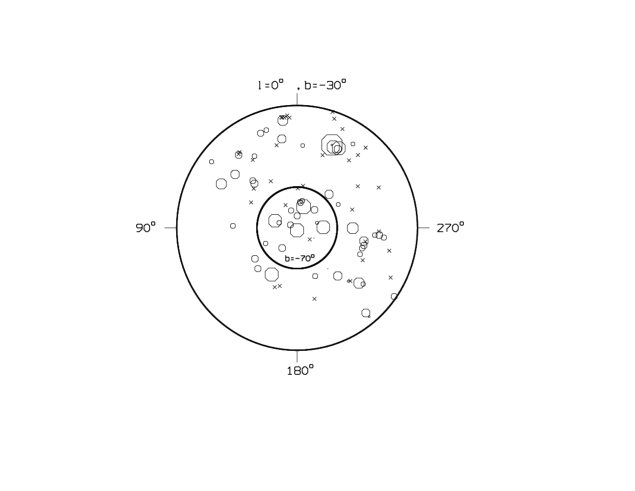
Figure 4: The distribution on the sky of the directions towards the 95 clusters with b$\leq$-30$\degr$ (see paper II). For 57 clusters a background density is known (circles) and the other 38 clusters for which no background density is known are indicated by crosses. The size of the circles reflects the background density.

As can be seen from Fig. 4, there is some structure in the distribution of the background values, in the sense that large values of $\sigma_{b}$ appear to cluster on scales of about 20 degrees, which corresponds about to 100 Mpc for z=0.1. However, around the south galactic pole, both high and low background values occur, and this is also the case around l $\simeq 338\degr$, b $\simeq-46\degr$. The latter concentration of high backgrounds corresponds to a supercluster mentioned in paper I; another, at l $\simeq 255\degr$, b $\simeq-54$ corresponds to the Horologium-Reticulum supercluster (Lucey et al., 1983), that was also mentioned in paper I.

3.4 Which profile fits best?

The MLM technique does not provide an absolute estimate of the probability that a distribution of galaxies is ‘produced’ by a certain type of profile. However, it does allow a comparison of the relative merits of different profiles, through the likelihood ratio statistic (see, e.g. Meyer 1975). If there are two alternative hypotheses that we are testing on a single data-set, the likelihood ratio statistic allows one to estimate the probability that the hypothesis with the lowest likelihood is false, under the assumption that the hypothesis with the highest likelihood is true.

In practice, one computes the statistic $-2\ln(L_{1}/L_{2})$ from the values of $-2\ln L$ given in Tables 4 to 7, for the different density profiles, taking one of the values of the likelihood found for a given data-set as a reference $L_{1}$, and comparing that to the likelihood $L_{2}$ found for the same data-set and a different profile. For large samples, the statistic $-2\ln L_{1}/L_{2}$ has a $\chi^{2}$ distribution with $n$ degrees of freedom, where $n$ equals the number of parameters not restricted by the null hypothesis.

In the present case, the parameters that are fixed for all density profiles (i.e. the centre position, the ellipticity and position angle) do not contribute to the degrees of freedom of the distribution, and $n=3$ because the core-radius (or characteristic radius) $r_{c}$, the slope $\beta$, and background density $\sigma_{b}$ are estimated independently for the different profiles. Note that the central density is not a free parameter, as it is constrained by the normalization implicit in the MLM technique.

In general, the likelihoods obtained from the fitting of the King profile are higher than those obtained from the fitting of the other profiles: in 37/45, 34/50 and 38/51 cases, respectively, comparing the King profile with the Hubble, NFW and de Vaucouleurs profiles. However, according to the likelihood ratio statistic the differences in the likelihood values obtained from fitting different profiles to the same cluster data-set, are generally not statistically significant (Fig. 5).

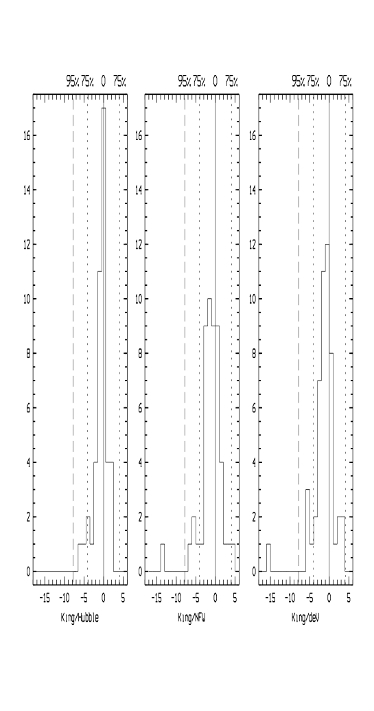
Figure 5: Distributions of $-2\ln L_{1}/L_{2}$ for the comparison between King and Hubble profiles (left), between King and NFW profiles (centre), and between King and de Vaucouleurs profiles (right). Negative values indicate that the first profile is preferred. We also show 95 $\%$ (long dash) and 75 $\%$ (short dash) significance levels. We note that for the right histogram, A3141 is out of the range with a value of -25.72.

If we set a 95 % significance level for rejection, and take the King profile as our null hypothesis, we do not reject the Hubble profile as inferior to the King profile for any of the clusters. For one cluster, A3528, the King profile provides a significantly better fit than the NFW profile, and for two clusters (A3128 and A3141) the de Vaucouleurs profile is rejected. There is, however, no cluster for which the Hubble, the NFW or the de Vaucouleurs profile provides a significant better fit than the King profile.

Most of the individual cluster density profiles, considered on the entire available area, do not allow us to select one of the four model profiles as the clear favorite and reject the others. However, in most cases the likelihood of the fit is highest when the King model is used. This may well be an indication that our inability to choose a particular model profile is due more to limited statistics than to a fundamental problem with the selection of a best-fitting profile. Moreover, we know that the shapes of the four profiles are very similar in the outer parts of the clusters, beyond 1 or 2 King core radii. The differences between for example a King and an NFW profile occur mainly in the very central parts of the clusters.

We have re-computed the statistic $-2\ln(L_{1}/L_{2})$ inside a square of 2 King core radii for the King and NFW profiles. In general, the differences between the fits are more significant in the inner regions: 32 out of 50 clusters show a better fit for the King profile at a confidence level of 99$\%$, while only 6 out of 50 yield a better fit for the NFW profile at the same confidence level. This again seems to point to the existence of a core in a large fraction of clusters of galaxies.

4 Density profiles of composite clusters

The result in $\S$ 3.4, viz. that the likelihood ratios for the King and NFW profile fits, when taken at face value, all indicate that the King profile provides a better fit than the NFW profile is quite tantalizing, although we realize full well that by themselves none of the likelihood ratios except one or two really indicate a highly significant preference for the King profile over the NFW profile. However, it cannot be excluded that the King profile in fact provides a better fit for a majority of our clusters, but that the limited statistical weight of the data for most of our clusters, when taken by themselves, prevents a significant demonstration of that fact. The fact that the King profile is preferred over the NFW profile in the central regions is quite interesting, because this result is obtained with smaller numbers of galaxies.

By combining the galaxy distributions for many clusters we have increased the statistical weight, in an attempt to get a more significant answer to the question if certain model profiles fit better than others, and particularly if galaxy distributions in clusters have cores or central cusps.

4.1 The construction of the composite clusters

The combination of the galaxy distributions of many clusters to produce what we will refer to as a composite cluster, requires a lot of care. In order not to smooth (or produce) possible cusps, and to avoid artefacts as a result of differences in sampling or due to the superposition of elongated, imperfectly centered galaxy distributions, we have used the following procedures.

First, we must account for the fact that different clusters have different ‘sizes’. If one were certain that all clusters obey the same type of projected galaxy density profile, with different ‘core radii’ to be sure, one could simply put the projected distances between the galaxies in all clusters on the same scale, by using the core radius to scale all projected distances before adding the galaxy distributions. However, one can also make a case for scaling by r₂₀₀, the radius within which the average density is 200 times the average density in the universe. According to Navarro, Frenk and White (1997), scaling with r₂₀₀ takes into account differences in mass. In the present discussion, we have produced composite clusters without scaling. Only for the comparison between the composite clusters, i.e. for getting an indication which profile best fits the composite clusters (see $\S$ 4.4), we have applied scaling.

A second result of the differences in characteristic scale is that the observations of the various clusters do not cover the same aperture, when expressed in core radius. To correct for this, we have applied a slightly modified version of the method devised by Beers and Tonry (1986), and by Merrifield & Kent (1989). The essence of that method is that one adds a model contribution to the observed data in the area where a particular cluster does not contain data, based on its relative contribution in the area where it does contribute. In practice, we combine the galaxy distributions of the clusters, beginning with the cluster with the largest and second largest core radii. We add some galaxies to the second largest cluster in the area where this cluster does not have data, according to the density profile that was fitted to the central region. For this ‘extrapolation’ we used the King-profile fit, but as all model profiles that we used have essentially the same outer logarithmic slope, the result would have been identical had we used e.g. the NFW profile fit. This process is repeated for all remaining clusters in order of decreasing core radius.

In this method there is an evident problem with the background. When we ”reconstruct” the profile as described above, the background galaxies are implicitly, and approximately taken into account. The reason for this is that the galaxies that are added in the outer regions of the smaller clusters, are added in proportion to the total number of galaxies, i.e. cluster members plus background galaxies. This causes the background to be not exactly ‘conserved’. However, it is not simple or even possible to do much better without redshift information. To estimate the background effect, we will build a composite cluster (see $\S$ 4.3) with only ENACS galaxies, for which the membership is clear from the redshift.

4.1.1 The effect of cluster elongation

We have taken the elongation of the clusters into account by ‘circularizing’ the individual galaxy distributions by increasing all projected distances orthogonal to the major axis by the appropriate factor, thus ‘expanding’ the distribution parallel to the minor axis. For this correction we used the ellipticities from Tab. 1. Even though the ellipticities of most of our clusters are not very large, this correction may be important because the superposition of elliptical galaxy distributions with randomly distributed orientations will cause the outer densities to be underestimated with respect to the inner ones, which may produce an artificial cusp (see Fig. 6).

Figure 6: Superposition of 4 elliptical clusters with different orientations of the major axes. The intensity of the shading is proportional to the number of contributing clusters.

We have checked the importance of the ellipticity correction by constructing two artificial composite clusters. Both are the superposition of 50 ‘perfect’, artificial King-profile clusters, each containing 100 galaxies in a 1200 kpc square aperture (without background). We assumed $\beta=1.0$ and selected r_c from a uniform distribution in the (50,150)-kpc interval. One composite cluster was made with an ellipticity distribution which mimics the observed one. I.e., we assumed 35 clusters to have $e$ uniformly distributed in the interval (0.0,0.1) and the other 15 uniformly in the interval (0.25,0.75). We assumed position angles to be randomly distributed between 0$\degr$ and 360$\degr$, which is fully consistent with the observations. For the first composite cluster, no correction for ellipticity was applied, the galaxy distributions were simply summed.

For the second artificial composite cluster we also used 50 clusters, again with $\beta=1.0$ and r_c from a uniform distribution in the (50,150)-kpc interval. However, in this case, all ellipticities were drawn uniformly from the range (0.0,0.1). In Fig. 7, we show the profiles of the two artificial composite clusters. As expected, the composite cluster with the real ellipticity distribution, and without correction for ellipticity, has a 2$\sigma$-excess in the very centre compared to the artificial cluster built from almost round clusters. Adding 15 elongated clusters thus induces a small but significant cusp.

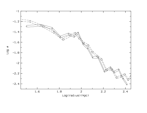
Figure 7: The two artificial composite clusters, each built from 50 ‘perfect’ King-profile clusters of 100 galaxies. The profile indicated by circles is the result of taking the observed ellipticity distribution, but without applying a correction for ellipticity. The profile indicated by crosses is the result of adding 50 clusters which are all practically round, making a correction for ellipticity unnecessary. Errors are shown as dashed and solid lines.

4.1.2 The effect of centering errors

Whereas neglecting the ellipticity correction produces an artificial cusp, errors in the central position will tend to destroy (if not totally, at least partly) a real cusp in a composite cluster, as argued by Beers and Tonry (1986). The magnitude of this effect depends fairly strongly on the ratio of the position errors and the core radii. We have tested the effect of errors in the centre position for our dataset, using again ‘perfect’, artificial NFW-profile clusters. We use 50 perfectly circular clusters with 100 galaxies each. The characteristic radii are uniformly distributed in the range (250,300) kpc.

We produce five composite clusters, the first with perfect centering and the other with random shifts of the real centres lower than 40 kpc, 65 kpc, 85 kpc, 125 kpc and with arbitrary orientation. The profiles for the two first artificial composite clusters are shown in Fig. 8, from which we conclude that there is indeed a smoothing due to the position errors, but it is very small. Therefore it is very unlikely that our results are seriously influenced by it. Actually, a 2-D Kolmogorov-Smirnov test indicates that the two artificial composite clusters are indistinguishable at a level of about 99%, but this result refers to the whole area, and not just the central part of the clusters. In order to quantify the effect of larger shifts, we have compared the quality of the NFW and King profile fitting for the 5 composite clusters through the likelihood ratio statistic (see Sec. 3.4). We find that the first 3 clusters (shifts of 0, 40 and 65 kpc), are significantly better fitted by a NFW profile than by a King profile at the 99$\%$ confidence level. A shift of 85 kpc provides also a better fitting for a NFW profile but only at the confidence level of 95$\%$. Finally, for shifts of 125 kpc, we have a slightly better fitting for a King profile, even if the difference is not significant. This shows that even if we attribute the entire difference between our isodensity centres and the ROSAT centres to errors in our centre positions (which is certainly an overestimation), those errors are not likely to have destroyed a potential cusp.

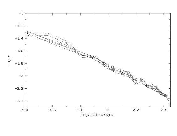
Figure 8: Superposition of the profiles calculated for composite clusters that were built from artificial clusters with NFW-profiles with true centres (solid line), with moderate centre shifts (40 kpc: short-dashed line) and large centre shifts (125 kpc: long-dashed line).

4.2 The COSMOS composite cluster

For the construction of the composite cluster based on COSMOS data, we have used the 29 clusters that we also used in our analysis of the Fundamental Plane of clusters (Adami et al. 1998). This subset of 29 clusters was selected from the sample of 62 clusters in Tab. 1 on the basis of the regular character of the galaxy distribution. For these 29 clusters, we have indicated in Fig. 1 the areas that we used in the construction of the composite cluster. It can be seen that these are free from evident substructures. In order to quantify this fact, we have applied a Dressler-Shectman test inside these areas. At a confidence level of 5$\%$, there are only 4 clusters among the 29 which show signs of substructures: viz. A1069, A2644, A3122 and A3128 (14 $\%$ of all the galaxies). If we exclude the Emission Line Galaxies only A1069, A2644 and A3128 show substructure. The contribution of these clusters is certainly minor and we considered the composite cluster essentially free from substructures. A3128, which is classified as multimodal, is included as its main peak is well-defined. The 29 clusters all have a redshift smaller than 0.1 and at least 10 redshifts in the area within 5 King core radii. In principle, the latter requirement is not important for the present discussion, but if one adds the 15 regular clusters from Tab. 1 with less than 10 redshifts, the total number of galaxies increases by only 13%.

From the 29 clusters with 4735 galaxies, we have constructed a composite cluster; in doing so we added 2505 galaxies in the outer parts of the smaller clusters (see $\S$ 4.1), to produce a cluster with 7240 COSMOS galaxies. The area where we fit the models on the composite cluster has a radius of 600 kpc, which is similar to that of the area over which the profiles of the individual clusters were fitted. For the present discussion no scaling of projected distances was performed. Although the dispersion of the characteristic scales is not very large (see $\S$ 3.2), the superposition of galaxy distributions with different scales may affect the profile of the composite cluster. For example, adding clusters with identical types of profile with small and large core radii might produce a cluster which does not have the same profile as the individual clusters from which is was built. When discussing the question of which type of profile best fits the observations (see $\S$ 4.4) we will therefore also discuss results for composite clusters for which the constituting clusters were scaled before adding them.

In Fig. 9 we show the result for the COSMOS composite cluster, for which all projected distances were scaled with the King and NFW characteristic radii of the individual clusters: we take the value predicted with the regression line between the King and NFW radii. We note here that the relation between these two radii is well defined (see $\S$ 3.2). The profile was calculated in radial bins which each contain 20 galaxies. The dashed lines indicate the 1-$\sigma$ range around the observed values (the dots). The two full-drawn curves represent the best King and an NFW fits. It is clear that the observed values within r_c (log r $<$ 0) indicate a flat profile. In $\S$ 4.4 we will discuss the result of a formal test of which of the two model profile best represents the three composite clusters. Looking at this figure, one may already get some idea about the outcome of that test.

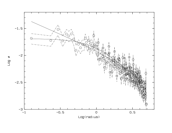
Figure 9: The projected density in the composite COSMOS cluster that was produced by scaling all projected distances with the core radii of the individual clusters, so the horizontal scale gives r/r_c. The dots give the observed values in bins which contain 20 galaxies each. The dashed lines indicate the 1-$\sigma$ interval on either side of the observed values. The full-drawn curves represent the King and an NFW profile.

Using the MLM method we fitted both a King and an NFW profile to the (unscaled) composite COSMOS cluster. These fits give: $\beta=1.00\pm 0.02$, r${}_{c}=89\pm 5$ and $\sigma_{b}=2.00\pm 0.03$ 10^-3 for the King profile, and $\beta=0.56\pm 0.01$, r${}_{c}=318\pm 34$ and $\sigma_{b}=1.44\pm 0.05$ 10^-3 for the NFW profile. The value of $\beta$ of 0.56$\pm$0.01 for the NFW-profile is somewhat lower than the value one would predict on the basis of the $\beta$ for the King-profile fit, using the expected relation between the two $\beta$’s. Imposing $\beta$ = 0.67 for the NFW profile, the fit is worse but we obtain $\sigma_{b}=1.70$ 10^-3, which is closer to the value found in the King-profile fit. This shows that $\beta$ and $\sigma_{b}$ are correlated.

The values of r_c, $\beta$ and $\sigma_{b}$ for the composite cluster are globally consistent with the average values found for the 62 clusters in $\S$ 3.2. The agreement is also good if we compare with the average values for the subsample of the 29 clusters used here rather than for the total sample. For the 29 clusters, the average values of $\beta$ and r_c and the value of $\Sigma\sigma{{}_{b}{{}_{i}}}$ are 1.04$\pm$0.08, 115$\pm$67 kpc, 1.17$\pm$0.56 10^-3 for the King-profile fits and 0.61$\pm$0.05, 276$\pm$181 kpc, 1.13$\pm$0.55 10^-3 for the NFW-profile fits.

If we restrict the fits to the central region (radius: 300 kpc) of the composite cluster (924 galaxies), we obtain $\beta$ = 1.02 and r_c = 106 kpc for the King profile and $\beta$ = 0.55, r_c = 272 kpc for the NFW profile. These values for the central region agree better with the values for the individual clusters; this may be partly due to the fact that the addition of galaxies in the outer regions of the clusters hardly affect the central region. But the relative importance of errors in the assumed centre positions or in the core radii determinations is probably larger.

We have also made a composite cluster fr om those 14 clusters for which a central position is available from ROSAT, using the latter centre rather than ours. We fit both a King and a NFW profile in a more central area (radius: 200 kpc) and find a better fit for the King profile at the 95$\%$ confidence level. The use of the ROSAT centres does not change our conclusion about which profile fits best.

4.3 The ENACS composite cluster

In principle, the ENACS data could have been used to make independent solutions for r_c and $\beta$ for the individual clusters. Because the ENACS data allow us to select cluster members through their redshifts, the backgrounds would, by definition, be zero. However, the ENACS data are limited to the central regions of the clusters, and redshifts are not available down to the magnitude limit of the COSMOS data. Therefore, the number of ENACS galaxies in a cluster is, in general, too small to make a reliable fit. By combining the ENACS data for all 21 clusters among the 29 for which the ENACS data cover a rectangular area of at least 400 kpc to a side we have constructed an ENACS composite cluster with 388 galaxies.

MLM fits to this composite cluster yield $\beta=1.00\pm 0.05$ and r${}_{c}=91\pm 12$ for the King profile and $\beta=0.51\pm 0.03$, r${}_{c}=274\pm 61$ for the NFW profile. When we impose $\beta$ = 0.67 for the NFW-profile fit leads to a value of the likelihood that is a factor 5 worse than the maximum likelihood. It is likely that the lower value of $\beta$ is, at least partly, due to the fact that the size of the aperture is fairly small compared to the value of r_c for the NFW-profile fit.

Although the statistical weight of the ENACS composite cluster is much less than that of the COSMOS composite cluster, the results of the 2-parameter, rather than 3-parameter, fit provide strong support for the profile parameters found in $\S$ 4.2.

4.4 Which profile best describes the observations?

Using the COSMOS composite cluster, we have again addressed the question posed in $\S$ 3.4. We use three different versions of the composite cluster: one without scaling (as in $\S$ 4.2), one in which all projected distance are scaled with the values of r_c for the individual clusters as derived in $\S$ 3.2 (and given in Tabs. 4 to 7), and one in which we scaled with the individual values of r₂₀₀. The latter were calculated from the ENACS velocity dispersions, following e.g. Carlberg et al. (1997). For all three composite clusters we have made fits with a King- and an NFW-profile model.

We thus derived three values for the likelihood ratio $-2\ln(L_{1}/L_{2})$. These are -17, -17 and -10 for unscaled, r_c-scaled and r₂₀₀-scaled composite clusters, respectively. All three values are negative, and thus indicate a preference for the King profile over the NFW profile. The formal associated significance levels are 99, 99 and 95 percent. So, at face value, the result of $\S$ 3.4 is confirmed and amplified: that the majority of our clusters are indeed better explained by King profiles than by NFW profiles.

The following caveats must, however, be remembered in connection with this conclusion.

First: there is a small smoothing effect due to the errors in the centre positions, which we cannot quantify very well (using the best-fit centres is the best that we can do). Secondly, our selection of clusters is certainly not unbiased: we have used the most regular clusters (which in general are among the most massive ones). This could produce a sample of well-evolved clusters, which need not be typical of the total rich cluster population as far as the galaxy density profile is concerned. Thirdly, the assumption underlying the composite clusters, namely that when properly scaled , all clusters have the same profile, may well be a simplification. Finally, the likelihood ratio for the two fits to the composite clusters with r₂₀₀-scaling is least indicative of a preference for a King profile over an NFW profile. This may be just a statistical effect, but it might also be an indication that the absence of scaling, or the r_c-scaling, cause some smoothing due to incorrect combination of profiles which, intrinsically, have a moderate cusp. The likelihood ratio for the r₂₀₀-scaling applies to a composite of the 7 clusters in which the data extend out to at least 0.75 r₂₀₀ (this cluster contains 1092 COSMOS galaxies).

4.5 The effect of absolute magnitude

Finally we calculate likelihood ratios for different ranges of absolute magnitude. The reason for this is that e.g. Carlberg et al. (1997) claim the existence of a central cusp for the bright galaxies in clusters. We use the COSMOS composite cluster and we fit King and NFW profiles in the central 300 kpc (radius), for different magnitude ranges. We define the following 4 intervals of absolute magnitude, which contain 200 galaxies each: (-22.4,-18.78), (-18.77,-18.03), (-18.02,-17.48) and (-17.47,-16.89). The likelihood ratios in these intervals are, +1, –8, –8 and –4, respectively. It is clear that the preference for a King profile is certainly not shared by the brightest galaxies.

We have tried to estimate the magnitude for which the galaxy profile seems to change character. Taking narrower intervals, which contain 50 galaxies each, we find that for absolute magnitudes brighter than -18.4$\pm$0.2 the likelihood ratio (or rather $-2\ln(L_{1}/L_{2})$) is about 0, while fainter than -18.4$\pm$0.2 we obtain values between -4 and -8. That bright and faint galaxies do not have the same distribution is not totally new. E.g., Biviano et al. (1996) and Dantas et al. (1997) find that the faint and the bright galaxies in the Coma cluster and in A3558 respectively, have different distributions. The bright galaxies are very concentrated around a few specific positions while the distribution of the faint ones is smooth, and without a cusp.

4.6 Comparison with results in the literature

From the discussions in $\S$ 3.4 and $\S$ 4.4 we conclude that the COSMOS and ENACS data are better fitted by a King profile (or more generally: a profile with a core) than by an NFW profile (or rather: a profile with a cusp). In other words: our data seem to suggest a logarithmic slope in the central cluster region that is flatter than –1. Admittedly, this conclusion is based primarily on the composite clusters, and therefore we cannot be sure that the conclusion is true for all of the individual clusters as well. On the other hand, the results of the discussion in $\S$ 3.4 suggest that the conclusion may well be valid for most of the individual clusters. In addition, there is some evidence that the intrinsically brighter galaxies have a more cusped profile than the fainter ones.

In the literature there are several results that seem to be at odds with our first conclusion. Beers and Tonry (1986) argue e.g. for the presence of cusps and Carlberg et al. (1997) concluded that the CNOC clusters at a redshift of $\approx$ 0.3 have galaxy density profiles that are quite consistent with the NFW profile. Both conclusions are based on composite clusters, and as we discussed in $\S$ 4.1 several details of the construction of a composite cluster influence the destruction of cusps or their artificial production. Neither Beers and Tonry, nor Carlberg et al. seem to have taken the elongation of the clusters into account. As we found in $\S$ 4.1.1, that may be (partly) responsible for the appearance of a small cusp. On the other hand, it is also possible (if not likely) that the differences are largely due to the fact that our galaxy samples extend to fainter absolute magnitudes. We note here that the limiting magnitude of the CNOC survey (Carlberg et al., 1997) matches well with the value given in $\S$ 4.5 for which the King and NFW profiles become equivalent.

Therefore, the apparent disagreement may be largely resolved by our second conclusion, viz. that the brighter galaxies have a more cusped distribution than the fainter ones. Incidentally, this latter conclusion would also seem to indicate that for our clusters, the errors in the centre positions are indeed sufficiently small that they do not erase the cusp in the distribution of the brighter galaxies.

The values that we find for r_c are consistent with the results obtained by Girardi et al. (1995) and Bahcall (1975). Our value for $\beta$ is only moderately consistent with that obtained by Lubin & Bahcall (1994), who found 0.8$\pm$0.1. This discrepancy may be due to the fact that these authors fit their profile in the outer regions (500 to 1500kpc), which may contain substructure.

Our values of r_c and $\beta$ are local (z $<$ 0.1), and our $\beta$ value can be compared with $\beta$ estimates for other epochs. Recently, Lubin and Postman (1996) have studied 79 distant clusters from the Palomar Distant Cluster Survey (PDCS) with estimated redshifts between 0.2 and 1.2, where the precision of the redshift estimation was 0.2. They found r${}_{c}=50$ kpc and $\beta=0.7$ using a King profile. Because they have estimated the background at 1.2 Mpc from the centre, their estimate of r_c is probably not very accurate, and we do not consider the difference between their and our value for r_c to be really significant.

If one accepts the formal error bars for $\beta$, the difference in the $\beta$ values for distant and nearby clusters would be significant. If the differences between the values of $\beta$ are real, this indicates a change of the outer slope of the density profile with redshift (Tab. 8), in a way that is consistent with global ideas about an increase of the concentration of the clusters with cosmological time. According to commonly adopted formation and accretion scenarios for clusters of galaxies, young clusters have a flatter density profile than older, more evolved clusters.

Table 8: $\beta$ values for different redshifts from the present study and the study of Lubin & Postman (1996).

redshift	0.07$\pm$0.05	0.3$\pm$0.1	0.6$\pm$0.1	1$\pm$0.2
$\beta$	1.02$\pm$0.08	0.73$\pm$0.17	0.74$\pm$0.17	0.68$\pm$ 0.40

5 Profile slope $\beta$ and $\Omega_{0}$

From the analysis in $\S$ 3.2, $\S$ 4.2 and $\S$ 4.3 it is clear that the outer slopes of the galaxy distributions of the individual (and composite) clusters are all very much consistent with a value of 1.0, for King- and Hubble-profile fits. In addition, there is satisfactory consistency with the $\beta$-values for NFW- and de Vaucouleurs-profile fits (certainly for the individual clusters). We therefore conclude that this result is quite robust.

Quite a few numerical simulations have appeared in the literature from which the average present-day slope of the density profiles that is predicted as a function of the initial fluctuation spectrum, the cosmological parameters etc., can be estimated. In the following, we compare our result for $\beta$ with predictions obtained by Walter and Klypin (1996), Jing et al. (1995), Crone et al. (1994) and by Navarro, Frenk and White (1995).

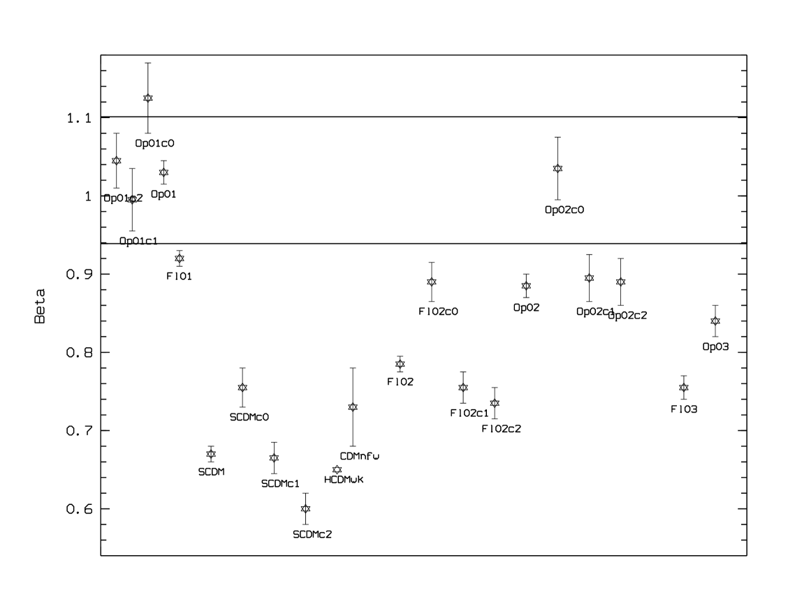
Figure 10: Numerical model values and observed values for $\beta$. The 2 straight lines define the range permitted with the invividual clusters.

Walter and Klypin (1996) simulate a mixed HCDM model with $\Omega_{CDM}=0.6$ and $\Omega_{\nu}=0.3$. The size of the simulation box is between 400 and 500 Mpc and they use the Harrison-Zeldovit’ch fluctuation spectrum. We will refer to it as the HCDMwk model.

Navarro, Frenk and White (1995, 1996) simulate a CDM model with $\Omega$ = 1.0. The size of the simulation box is 180 Mpc. We will refer to it as the CDMnfw model.

Jing et al. (1995) simulate seven scenarios, in 128 Mpc boxes. Each model gives more than 50 clusters which is very similar to our real sample. The fluctuation spectrum is the Harrison-Zeldovit’ch one. The models are: a standard CDM model with $\Omega_{0}=1$ (SCDM), three flat models with $\Omega_{0}=0.1$, 0.2 and 0.3 (with $\Lambda$ = 0.9, 0.8 and 0.7, respectively) (Fl01, Fl02 and Fl03) and three open models with $\Omega_{0}=0.1$, $0.2$ and 0.3, and $\Lambda$ = 0 (Op01, Op02 and Op03).

Crone et al. (1994) simulate three models with $\Omega_{0}=0.1$ and 0.2 using different fluctuation spectra: P(k)$\propto$k⁰, k and k². The models are three standard CDM ones (SCDMc0, SCDMc1 and SCDMc2), three flat universes with $\Omega_{0}=0.2$ and $\Lambda$ = 0.8 (Fl02c0, Fl02c1 and Fl02c2), three open universes with $\Omega_{0}=0.1$ (Op01c0, Op01c1 and Op01c2) and three open universes with $\Omega_{0}=0.2$ (Op02c0, Op02c1 and Op02c2).

All four groups fit 3-D power laws r${}^{-2\beta_{3D}}$ to the outer regions of the clusters, at the present-epoch which corresponds very well to the redshift range of our clusters. Their values are transformed to 2-D values, as follows: $\beta_{2D}=\frac{2\beta_{3D}-1}{2}$. We compare these 2-D model values with our observed mean $\beta_{2D}=1.02\pm 0.08$ for the King-profile fit in Fig. 10.

We find that only fairly low values of $\Omega_{0}$ produce average values for $\beta_{2D}$ that are similar to the observed value; this is in agreement with other recent results on $\Omega_{0}$. However, not all low-$\Omega_{0}$ models produce the observed value of $\beta_{2D}$. Taking the results in Fig. 10 at face value, it would seem that not only needs $\Omega_{0}$ to be small (a few tenths), but it is also not likely that we need to invoke a flat Universe (i.e. a non-zero value for $\Lambda$). The only exception to this general conclusion seems to be the flat model with $\Omega_{0}$ = 0.2 and a fluctuation spectrum P(k)$\propto$k⁰.

It should be realized that the conclusion that $\beta_{2D}$ is best predicted by low-$\Omega_{0}$ models (and possibly mostly open models ) is based on a rather incomplete range of models. In other words: we cannot exclude models that have not yet been calculated or published. E.g. it is too early to firmly exclude HCDM models with other fluctuation spectra than the one calculated by Walter and Klypin. On the other hand, the data in Fig. 10 seem to suggest that for $\beta$ the influence of the fluctuation spectrum is quite limited, so our conclusion of a low-$\Omega_{0}$ model (most likely open) is probably quite robust.

This value of $\Omega_{0}$ from the outer slope of the projected galaxy distribution can be compared to direct estimates of $\Omega_{0}$ based on cluster masses and luminosities and the field luminosity density. The idea is quite simple: one estimates the cosmological volume which contains the same mass as that contained in the cluster, from a comparison of the luminosity density in the field and the total luminosity of the galaxies in the cluster. This yields the average mass density which yields $\Omega_{0}$ through division by the critical density $\rho_{c}$. In practice, the method amounts to calculating the ratio of the $\frac{M}{L}$ ratio in cluster to the critical $\frac{M}{L}$ ratio in the field, and this result does not depend on $H_{0}$. A recent application of the method was discussed by Carlberg et al. (1996) for their sample of 16 clusters at a redshift of $\approx$ 0.3.

We have determined luminosities and velocity dispersions for our sample of 29 ENACS clusters discussed in paper IV. The luminosities and dispersions are calculated in an aperture of five core radii. We derived the projected virial masses (e.g. Perea et al. 1990) and obtained the $\frac{M}{L}$ ratios for the 29 clusters. The values of $\frac{M}{L_{b_{j}}}$ of the 29 clusters range from about 100 to 1000; the average value is 454, the median is 390 and the robust bi-weight estimate of the mean is 420, in good agreement with the value given by e.g. Bahcall et al. (1995). The local critical $\frac{M}{L}$ ratio in the field was determined by e.g. Efstathiou et al. (1988) and Loveday et al. (1992), who find a best estimate of 1500 $\frac{M_{\odot}}{L_{\odot b_{j}}}$, with the value most probably in the range 1100 to 2200. This yields an estimate of $\Omega_{0}$ on the basis of our sample of 29 local ENACS clusters of 0.28 $\pm$ 0.19. This value is thus quite consistent with the low $\Omega_{0}$ value that we obtained from the outer slopes of the projected galaxy distributions.

The uncertainty in the ‘dynamical’ $\Omega_{0}$ estimate is to a large extent due to the large spread in $\frac{M}{L}$ ratios for our clusters. It appears that the individual values of $\frac{M}{L}$ correlate moderately well with velocity dispersion, in accordance with the result in paper IV. Expressed in $\Omega_{0}$ we find: $\Omega_{0}$ = (3.9$\pm$1.1) 10^-2 $\sigma_{v}/100$ + (8$\pm$157)10^-3. If we use the relation between luminosity, scale factor and velocity dispersion that we derived in paper IV we obtain: $\Omega_{0}$ = (3.2$\pm$0.5) 10^-4 $\sigma_{v}^{1.09}$ $R^{-0.19}$, which is totally consistent. It thus appears that there is a significant dependence on cluster velocity dispersion in the determination of $\Omega_{0}$ from cluster $\frac{M}{L}$ ratios, which could easily produce a serious bias towards high values.

Of course, we have assumed in this analysis that in clusters light traces mass. Actually, this assumption is not really demonstrated, but is commonly used, for example in Carlberg et al. (1996). One might wonder how this assumption could affect our last $\Omega_{0}$ estimate. However, for the low $\sigma_{v}$ clusters, the present estimate is in good agreement with that based on the slope of the density profiles, and that gives some confidence that a possible bias is probably quite small.

6 Conclusions

We have studied the projected galaxy distributions in 77 clusters from the ESO Nearby Abell Cluster Survey. The present sample is an unbiased subset of the volume-limited ENACS sample, and thus forms a representative local (z $<$ 0.1) sample of rich (R_ACO $>$ 1), optically selected clusters. We used both COSMOS and ENACS data to test the character of the projected galaxy distributions. In particular, we have investigated whether the galaxy distributions in rich clusters have cusps or cores in their central regions.

We have made maximum Likelihood fits to the observed distribution of COSMOS galaxies to solve for the position and the elongation of the clusters. For 15 of the 77 clusters, no reliable centre could be determined and these clusters were not considered further. Using the positions and elongations, we subsequently solved for each of the 62 remaining clusters the three parameters that describe each of the four theoretical profiles that we tested, as well as the density of background galaxies. The four model profiles that we tested against the data are the King, Hubble, NFW (Navarro, Frenk and White) and the de Vaucouleurs profiles. Although the solutions do not converge for all of the clusters nor for all four profiles, we obtain reliable results for between 75 and 95 % of the clusters (depending on the model profile).

We find mean values for r_c, the characteristic scale of the 2-D galaxy distribution, and dispersions around the means of 128 $\pm$ 88, 189 $\pm$ 116, 292 $\pm$ 191 and 1582 $\pm$ 771 kpc, for the King, Hubble, NFW and de Vaucouleurs profiles respectively. The outer logarithmic slopes of the distributions were generalized by the usual $\beta$-parameter, which we find to have the following average values: 1.02 $\pm$ 0.08, 1.03 $\pm$ 0.07, 0.61 $\pm$ 0.05 and 7.6 $\pm$ 0.5, for the King, Hubble, NFW and de Vaucouleurs profiles respectively, which are consistent. The average background density at the limit of the COSMOS catalogue is about 4 10^-5 galaxies arcsec^-2.

In order to investigate whether the galaxy distributions in our clusters preponderantly have cores or cusps, we have determined the likelihood ratio for the King and NFW profiles. Using all galaxies down to the COSMOS magnitude limit of about m${}_{b_{j}}$ $\approx$ 19.5, we find that in general the King profile is more likely to be a good representation of the data than the NFW profile. However, for the individual clusters this preference for the King profile is generally not statistically significant. If we restrict the analysis to the central regions, the significance of the preference for the King-profile fits increases, even though the number of galaxies decreases.

We have increased the statistical weight for the likelihood analysis by combining the galaxy distributions in a subset of 29 of the 62 clusters, which show a regular galaxy distribution. We take special care to avoid the creation of an artificial cusp (by taking the ellipticities into account), and to avoid the destruction of a real cusp by summing distributions with different scale lengths. We have also checked that it is unlikely that the uncertainty in the centre positions has erased a cusp. For the test we summed without scaling projected distances, after scaling with r_c, as well as with r₂₀₀. In all three cases we find that the King profile provides a better fit to the data than the NFW profile, at confidence levels of more than 95 %. Interestingly, this preference is not shared by the brighter galaxies.

Finally, we have used the outer profile slope (i.e. the result that $\beta$ is very close to 1.0), in combination with several results from numerical models to conclude that the density parameter $\Omega_{0}$ is likely to be considerably smaller than unity. In addition, the available models indicate that the Universe probably has an open geometry (i.e. no closure through $\Lambda$ is indicated). This low implied value of $\Omega_{0}$ is fully consistent with a direct determination based on the $\frac{M}{L}$ ratios of our clusters.

- [1] Adami C., Mazure A., Biviano A., Katgert P., Rhee G., 1998, A&A 331, 493: paper IV
- [2] Arnouts S., de Lapparent V., Mathez G., et al., 1997, A&AS 124, 163
- [3] Bahcall N.A., Lubin L.M., Dorman V., 1995, ApJ 447, L8
- [4] Bahcall N.A., 1975, ApJ 198, 249
- [5] Beers T.C., Flynn K., Gebhardt K., 1990, AJ 100, 32
- [6] Beers T.C., Tonry J.L., 1986, ApJ 300, 557
- [7] Bellanger C., de Lapparent V., Arnouts S., et al., 1995, A&AS 110, 159
- [8] Biviano A., Durret F., Gerbal D., et al., 1996, A&A 311, 95
- [9] Biviano A., Katgert P., Mazure A., et al., 1997, A&A 321, 84: paper III
- [10] Carlberg R.G., Yee H.K.C., Ellingson E., et al., 1996, ApJ 462, 32
- [11] Carlberg R.G., Yee H.K.C., Ellingson E., et al., 1997, ApJ 485, L13
- [12] Colless M., 1989, MNRAS 237, 799
- [13] Colless M., Hewett P., 1987, MNRAS 224, 453
- [14] Crampton D., Le Fevre O., Lilly S.J. et al., 1995, ApJ 455, 96
- [15] Crone M.M., Evrard A.E., Richstone D.O., 1994, ApJ 434, 402
- [16] Dantas C.C., de Carvalho R.R., Capelato H.V., Mazure A., 1997, ApJ 485, 447
- [17] den Hartog R., Katgert P., 1996, MNRAS 279, 349
- [18] de Theije P.A.M., Katgert P., 1998, A&A submitted: paper VI
- [19] de Theije P.A.M., Katgert P., van Kampen E., 1995, MNRAS 273, 30
- [20] Efstathiou G., Ellis R.S., Peterson B.A., 1988, MNRAS 232, 431
- [21] Fletcher R., 1970, Comput. J. 13, 317
- [22] Girardi M., Biviano A., Giuricin G., Mardirossian F., Mezzetti M., 1995, ApJ 438, 527
- [23] Hernquist L., 1990, ApJ 356, 359
- [24] Heydon-Dumbleton N.H., Collins C.A., MacGillivray H.T., 1989, MNRAS 238, 379
- [25] Hughes J.P., 1997, To appear in ”A New Vision of an Old Cluster: Untangling Coma Berenices” astro-ph 9709272
- [26] Jing Y.P., Mo H.J., Borner G., Fang L.Z., 1995, MNRAS 276, 417
- [27] Katgert P., Mazure A., den Hartog R., et al., 1998, A&A accepted: paper V
- [28] Katgert P., Mazure A., Perea J., et al., 1996, A&A 310, 8 : paper I
- [29] King I.R., 1962, AJ 67, 471
- [30] Kofman L., Klypin A., Pogosyan D., Henry P., 1996, ApJ 470, 102
- [31] Lilly S.J., Le Fevre O., Crampton D., Hammer F., Tresse L., 1995, ApJ 455, 50
- [32] Loveday J., Peterson B.A., Efstathiou G., Maddox S.J., 1992, ApJ 390, 338
- [33] Lubin L.M., Bahcall N.A., 1994, ApJ 426, 513
- [34] Lubin L.M., Postman M., 1996, AJ 111, 1795
- [35] Lucey J.R., Dickens R.J., Mitchell R.J., Dawe J.A., 1983, MNRAS 203, 545
- [36] Mazure A., Katgert P., den Hartog R., et al., 1996, A&A 310, 31 : paper II
- [37] Merrifield M.R., Kent S.M., 1989, AJ 98, 351
- [38] Meyer S.L., 1975, ”Data Analysis for Scientists and Engineers”, p.352, John Wiley & Sons, New York
- [39] Michie R.W., Bodenheimer P., 1963, MNRAS 126, 269
- [40] Navarro J.F., Frenk C.S., White S.D.M., 1995, MNRAS 275, 720
- [41] Navarro J.F., Frenk C.S., White S.D.M., 1996, MNRAS 462, 563
- [42] Navarro J.F., Frenk C.S., White S.D.M., 1997, ApJ 490, 493
- [43] Nelder J.A., Mead R., 1965, Comput. J. 13, 317
- [44] Perea J., Del Olmo M., Moles M., 1990, A&A 237, 319
- [45] Plionis M., Barrow J.D., Frenk C.S., 1991, MNRAS 249, 662
- [46] Sarazin C.L., 1980, ApJ 236, 75
- [47] Silverman B., 1986, Density Estimation for Statistics and Data Analysis, London: Chapman and Hall
- [48] Teague P.F., Carter D., Gray P.M., 1990, ApJS 72, 715
- [49] van Albada T.S., 1982, MNRAS 201, 939
- [50] van Kampen E., 1995, MNRAS 273, 295
- [51] Walter C., Klypin A., 1996, ApJ 462, 13