Measuring Distances Using Infrared Surface Brightness Fluctuations

Abstract

Surface brightness fluctuations (SBFs) are much brighter in the infrared than they are at optical wavelengths, making it possible to measure greater distances using IR SBFs. We report new ${K^{\prime}}$ (2.1µm) SBF measurements of nine galaxies in the Fornax and Eridanus clusters using a 1024²-pixel HgCdTe array. We used improved analysis techniques to remove contributions to the SBFs from globular clusters and background galaxies, and we assess the relative importance of other sources of residual variance. We applied the improved methodology to our Fornax and Eridanus images and to our previously published Virgo cluster data. Apparent fluctuation magnitudes were used in conjunction with Cepheid distances to M31 and the Virgo cluster to calibrate the ${K^{\prime}}$ SBF distance scale. We find the absolute fluctuation magnitude ${\overline{M}_{K^{\prime}}}\,{=}\,{-}5.61\,{\pm}\,0.12$, with an intrinsic scatter to the calibration of 0.06 mag. No statistically significant change in $\overline{M}_{K^{\prime}}$ is detected as a function of $(V{-}I)$. Our calibration is consistent with simple (constant age and metallicity) stellar population models. The lack of a correlation with $(V{-}I)$ in the context of the stellar population models implies that elliptical galaxies bluer than ${(V{-}I)}\,{=}\,1.2$ have SBFs dominated by younger (5–8 Gyr) populations and metallicities comparable to redder ellipticals. Significant contributions to the SBFs from anomalous populations of asymptotic giant branch stars are apparently uncommon in giant ellipticals. ${K^{\prime}}$ SBFs prove to be a reliable distance indicator as long as the residual variance from globular clusters and background galaxies is properly removed. Also, it is important that a sufficiently high signal-to-noise ratio be achieved to allow reliable sky subtraction because residual spatial variance can bias the measurement of the SBF power spectrum.

1 Introduction

Because the light from a distant galaxy comes from discrete but unresolved stars, Poisson statistics lead to mottling of the galaxy’s otherwise smooth surface brightness profile. Surface brightness is independent of distance, but the amplitude of the surface brightness fluctuations (SBFs) is not. As the distance ($d$) to a galaxy increases, the number of stars ($n$) in a given resolution element increases as $d^{2}$, but the observed flux ($f$) from each star is reduced by $d^{-2}$, making surface brightness ($nf$) independent of distance. On the other hand, the rms variation in observed flux from region to region is $n^{1/2}f$, which scales as $d^{-1}$. The variance in surface brightness $nf^{2}$ normalized by the mean galaxy brightness $nf$ decreases with distance; distant galaxies appear smoother than nearby galaxies. Because the variance in surface brightness is proportional to the second moment of the stellar luminosity function, it is dominated by luminous red giant stars.

Although individual stars are not resolved, measuring SBFs probes the stellar population of the galaxy directly. With good theoretical models for stellar populations, the absolute magnitude of SBFs can be calculated, allowing a direct determination of the distance that is independent of the global dynamics or the environment of the galaxy (to the extent that the stellar populations in old stellar systems are independent of these variables). Alternatively, measuring SBFs in galaxies with known distances provides insight into stellar populations, allowing comparison with stellar evolution models and providing an empirical calibration of the SBF distance scale. Good descriptions of the theory and practice of using SBFs as a distance measurement tool and stellar population probe can be found in several papers by Tonry and collaborators (Tonry et al. 1997; Jensen, Luppino, & Tonry 1996, hereafter JLT; Tonry 1991; Tonry, Ajhar, & Luppino 1990; Tonry & Schneider 1988), in papers by Sodemann & Thomsen (1995, 1996), and in the review by Jacoby et al. (1992). The first $K$-band SBF studies are described by JLT, Luppino & Tonry (1993), and Pahre & Mould (1994).

J. Tonry and coworkers have completed an extensive survey of $I$-band SBF distances in a sample of several hundred early-type (dynamically hot elliptical and S0) galaxies which is more than 50% complete out to $\sim$2800 km s^-1 (Tonry et al. 1997). They find that the $I$-band absolute fluctuation magnitude $\overline{M}_{I}$ is a linear function of $(V{-}I)$ and has a universal zero point. Their $I$-band calibration, which is based empirically on Cepheid distances, is in good agreement with Worthey’s (1993a,b; 1994) simple stellar populations models. Worthey’s models predict that the effects of age and metallicity in the $I$ band are largely degenerate, so that $\overline{M}_{I}$ may be calibrated using a single parameter such as the $(V{-}I)$ color. The resulting intrinsic scatter of the $I$-band SBF distance scale is of order 0.07 mag. The purpose of the current study is to examine the behavior of the SBF calibration in the near-IR ${K^{\prime}}$ band, where Worthey’s models predict a much weaker dependence on $(V{-}I)$, but potentially larger scatter as the effects of age and metallicity are no longer degenerate.

Stellar surface brightness fluctuations are very red, since they are dominated by luminous red giant stars. The advantages of observing IR SBFs are clear: fluctuations are ${\sim}33$ times brighter at $K$ than at $I$, making them observable to greater distances. The SBF amplitude is inversely proportional to the seeing FWHM, and the seeing is typically much better in the IR than at optical wavelengths. Fluctuations are also red compared to the globular cluster (GC) population, so the contrast between stellar SBFs and GCs is higher at $K$. Finally, stellar population models predict that $K$-band SBF magnitudes have a much weaker dependence on $(V{-}I)$ than at $I$, reducing or eliminating the need to accurately measure the color of the galaxy (Worthey 1993a).

Several studies have demonstrated the feasibility of measuring IR SBFs, including Luppino & Tonry (1993), Pahre & Mould (1994), and JLT. These papers report results for a rather limited set of galaxies in the Local Group (LG) and the Virgo Cluster, but the consistency in the measured calibration of $\overline{M}_{K}$ is encouraging (${\overline{M}_{K^{\prime}}}\,{=}\,{-}5.61\,{\pm}\,0.16$ Luppino & Tonry, $M_{K_{sh}}\,{=}\,{-}5.77\,{\pm}\,0.18$ Pahre & Mould, ${\overline{M}_{K^{\prime}}}\,{=}\,{-}5.62\,{\pm}\,0.29$ JLT). All three of these papers report absolute fluctuation magnitudes that are consistent with Worthey’s (1994) predictions based on simple stellar population models. While the mean $\overline{M}_{K^{\prime}}$ of JLT and Pahre & Mould (1994) are quite consistent, differences in apparent fluctuation magnitudes for individual galaxies are larger than the stated uncertainties allow. JLT discuss several possible reasons for the disagreement in fluctuation magnitudes and showed that residual variance resulting from spatial variations in the detector sensitivity and dark current can contribute significantly to the power spectrum in low signal-to-noise ratio ($S/N$) observations. A residual pattern of only 0.1% of the sky level can significantly change the fluctuation magnitude measured. To use IR SBFs as a reliable distance indicator, it is critical that the observations be of sufficiently high $S/N$ ratio to avoid biases from residual variances. JLT also demonstrated that properly subtracting the sky and carefully sampling the point spread function (PSF) are crucial to accurately measuring the fluctuation amplitude. An uncertainty in the background subtraction of 2% of the sky level can dominate the uncertainty in the fluctuation magnitude.

Our Virgo sample showed a large dispersion (0.29 mag) due to the depth of the cluster and observational errors. Pahre & Mould (1994) also addressed the dispersion in fluctuation magnitude in a similarly-sized sample of Virgo ellipticals. Clearly a larger sample of galaxies is needed to calibrate the IR SBF distance scale. To better understand the effects stellar populations have on the fluctuation amplitude, we observed five galaxies in the Fornax cluster. Fornax is ideal for several reasons: first, it is much more centrally concentrated than the Virgo cluster. The reduced dispersion in distances allows us to better quantify and understand the uncertainty in our SBF measurements. Second, Fornax contains a large number of giant elliptical galaxies with a wide range of $(V{-}I)$ colors, metallicities, and globular cluster populations. The Virgo galaxies observed by JLT and Pahre & Mould (1994) spanned a very limited range in Mg₂ index to avoid stellar population variations which may affect the calibration of $\overline{M}_{K}$. We now extend the sample to calibrate ${K^{\prime}}$ fluctuation magnitudes across a wider range of metallicities and $(V{-}I)$ colors to compare with theoretical stellar population models. Finally, Cepheid distances to several Virgo cluster galaxies and to the Fornax spiral NGC 1365 have been measured using the Hubble Space Telescope (HST). We can empirically anchor our ${K^{\prime}}$-band SBF calibration both to the Cepheid and the $I$-band SBF distance scales.

This paper reports results from our observations of four Eridanus cluster elliptical galaxies in addition to the Fornax galaxies. Eridanus is not as compact a cluster as Fornax, but we can still compare our IR SBF results with the $I$-band results from Tonry (1997). Finally, we return to our SBF measurements for the seven Virgo ellipticals discussed by JLT and apply the improved techniques we describe in this paper. We present the updated results for these galaxies in Section 4.2, along with new observations of NGC 4365.

2 Observations and Data Reduction

2.1 Observations

This paper presents results derived from data obtained during several observing runs using the QUIRC camera mounted at the f/10 focus of the University of Hawaii 2.24 m telescope. QUIRC is a near-IR camera employing the first- and second-generation $1024^{2}$-pixel HgCdTe “HAWAII” detectors (Hodapp et al. 1996). These observations are compared to previous work which used the 256²-pixel NICMOS detector (JLT, Luppino & Tonry 1993). The second-generation science-grade HAWAII array has far fewer bad pixels, higher quantum efficiency, and a much more spatially uniform response than the earlier HgCdTe devices. The dark current for these detectors is less than 1 e^-s^-1 and the readnoise is $\sim$15 e^-. The QUIRC camera has a plate scale of 0$\farcs$1886 pixel^-1, providing a field of view 3$\farcm$2 on a side. The University of Hawaii ${K^{\prime}}$ filter used for these observations is centered at a slightly shorter wavelength (2.11 µm) than the standard $K$ filter to reduce the thermal background (Wainscoat & Cowie 1992). The mean sky background measured using the ${K^{\prime}}$ filter during this run was 13.4 mag arcsec^-2. These observations are directly comparable to those of JLT and Luppino & Tonry (1993), which used the same ${K^{\prime}}$ filter.

Table 1: SBF Observing Runs

Observation	Camera/	Scale	Field of view	Gain	Galaxies/clusters
dates	detector	(″)	(′)	(e-/ADU)
1993 Apr 7–11	NICMOS	0.375	1.6	30	Virgo
1995 May 17–20	QUIRC-1	0.19	3.2	6	NGC 4365, 4489
1995 Oct 14–17	QUIRC-1	0.189	3.2	6	Fornax, Eridanus
1996 Mar 1, Apr 27–28	QUIRC-2	0.189	3.2	1.85	NGC 4365

We observed five giant elliptical galaxies in the Fornax cluster and four in the Eridanus cluster over a period of four nights in 1995 October using the first-generation 1024²-pixel array. In this paper we reanalyze the Virgo cluster data originally presented by JLT. Most of the Virgo observations were made using the smaller $256^{2}$-pixel NICMOS3 array (Hodapp, Rayner, & Irwin 1992). Two of the JLT galaxies were observed using the first-generation 1024²-pixel array in the QUIRC camera. NGC 4365 was observed again in 1996 March and April using the second-generation $1024^{2}$-pixel HgCdTe array with improved electronics, and we compare these newer data to those presented by JLT. Details of the individual observing runs are presented in Table 1.

2.2 Preliminary Image Analysis and Reduction

Table 2: Photometric Data

Galaxy	$m_{1}$	$\sec z$	$A_{atm}$	Seeing	Sky	Resid. sky	$t_{exp}$	$t_{tot}$	$A_{B}$
NGC			(${{\rm mag}\over{\sec z}}$)	(″)	(mag/□″)	(e-s-1pix-1)	(s)	(s)	(mag)
Fornax
1339	$23.43\pm 0.10$	1.676	0.13	0.68	13.57	$-0.25\pm 0.10$	60	2160	0.00
1344	$23.36\pm 0.05$	1.635	0.10	0.74	13.15	$-0.63\pm 0.20$	60	2220	0.00
1379	$23.38\pm 0.10$	1.906	0.13	0.83	13.47	$-0.27\pm 0.17$	90	2070	0.00
1399	$23.19\pm 0.10$	1.888	0.13	0.83	13.21	$-0.73\pm 0.33$	90	1710	0.00
1404	$23.36\pm 0.05$	1.901	0.10	0.77	13.37	$-0.80\pm 0.15$	60	1980	0.00
Eridanus
1395	$23.19\pm 0.10$	1.621	0.13	0.75	13.05	$-0.63\pm 0.10$	90	1350	0.02
1400	$23.36\pm 0.05$	1.591	0.10	0.70	13.34	$-0.40\pm 0.20$	60	1980	0.13
1407	$23.38\pm 0.10$	1.550	0.13	0.91	13.56	$-0.66\pm 0.10$	120	2280	0.16
1426	$23.38\pm 0.10$	1.865	0.13	0.89	13.61	$-0.53\pm 0.10$	90	1710	0.02
Virgo W
4365	$22.91\pm 0.03$	1.000	0.00	0.59	13.30	$-0.73\pm 0.21$	89	2670	0.00

The techniques we used to do the initial data reduction are described by JLT. We adopted several key improvements for the new data described in this paper. Flat field images and bad pixel masks were created as described by JLT. To improve the noise characteristics of the background for our SBF analysis, we constructed average (rather than median) sky frames from ${\sim}6$ individual sky images which were interspersed with the galaxy observations. Stars were removed from individual images and bad pixels masked, and the remaining good pixels averaged to form the sky frame. The average sky frame was subtracted from individual galaxy images prior to flat fielding and removal of bad pixels and cosmic rays. The cleaned and flattened galaxy images were then registered to the nearest integer pixel and the good pixels averaged as described by JLT. Sub-pixel registration was not used because such procedures produce noise that is correlated from pixel to pixel and is therefore not constant with wavenumber in the power spectrum.

To calibrate the photometry, we frequently observed the faint UKIRT standards (Casali & Hawarden 1992). The majority of our 1995 October observations were made when conditions were not photometric. The photometric zero point fluctuated by as much as 0.25 mag during periods of all but one of the nights. To better calibrate our photometry, we compared our results to photoelectric aperture photometry (Persson, Frogel, & Aaronson 1979, Frogel et al. 1978, Persson et al. 1980). We measured the difference between our magnitudes and the photoelectric magnitudes for all galaxies in common (7 of 9) and used the mean difference and standard deviation to adjust our photometric zero-point and uncertainty for each night. Atmospheric extinction coefficients were determined by combining standard star observations covering a range of air masses during photometric periods of different nights. No color term to the photometry was measured. Photometric zero-points and extinction coefficients are listed in Table 2.

Next, we corrected for galactic extinction. From Cohen et al. (1981) we learn that

$$A_{V}:A_{K}:E(B-V)=3.04:0.274:1.00.$$ (1)

Following Tonry et al. (1997), we take $A_{V}/E(B{-}V)\,{=}\,3.04$ for early type galaxies. We assume that the extinction at $K$ and ${K^{\prime}}$ are the same, so combining the above relations gives $A_{{K^{\prime}}}\,{=}\,0.068A_{B}$. Values for $A_{B}$ are listed in Table 2 (Burstein & Heiles 1984).

No K corrections were needed for the low-redshift galaxies in this study. In Section 5.2 we describe stellar population models used to predict fluctuation magnitudes (Worthey 1994, 1997). The Worthey models were also used to determine the redshift dependence of the $K$-band fluctuation magnitudes. At a redshift of $z\,{=}\,0.005$ appropriate for the Virgo, Fornax, and Eridanus clusters, the K correction to the $K$-band fluctuation magnitude is $-0.001$ mag for a 17 Gyr stellar population and +0.004 for an 5 Gyr population ([Fe/H] = 0). While these corrections are for the $K$ filter, the offsets are so small that it is safe to assume the corrections to the ${K^{\prime}}$ SBF magnitudes are negligible. Even at redshifts of $z\,{=}\,0.025$ (7500 km s^-1), Worthey’s models predict corrections no larger than $\pm 0.015$ mag between ages of 5 and 17 Gyr. The fact that $K$ SBFs change so little as a function of redshift is very encouraging. The purpose of calibrating ${K^{\prime}}$ SBFs is to allow SBF measurements to be made to much larger distances than possible at $I$ band, and the absence of significant K corrections reduces the uncertainty in doing so.

3 Surface Brightness Fluctuation Analysis

3.1 Measuring SBF Magnitudes

We followed the same procedures described by JLT to measure SBF amplitudes in this data, with important modifications to account for the contributions from undetected globular clusters and background galaxies. We used the VISTA image analysis software (written by T. Lauer and R. Stover) and additional programs written by J. Tonry to perform the SBF analysis. The first step in the process was to determine the residual sky background remaining after stacking individual images. We assumed that this small adjustment (typically ${\lesssim}0.2\%$ of the sky level) was constant over the entire frame and could be applied as an offset to the final flattened and registered image. As JLT found, however, the fluctuation power is quite sensitive to residual patterns in sky subtraction, flat fielding, and non-zero background offsets, even at the level of ${\sim}0.1\%$ of the sky level. We estimated the residual sky background levels in the final images by fitting a deVaucouleurs $r^{1/4}$ profile to each galaxy using elliptical apertures. The larger QUIRC field of view made it possible to determine the residual sky level much more accurately than using NICMOS. The sky levels in the JLT data were also remeasured for consistency.

The next step in measuring the SBF magnitude was to fit and subtract the galaxy profile. We used a routine which allows the center, ellipticity, and position angle to vary as we fit annuli of increasing radius, and we iterated the procedure to ensure that the fit was well-behaved. Point sources were masked before fitting the galaxy profile. The resulting model of the galaxy was subtracted from the data. Large-scale residual background variations were also fitted and subtracted, leaving a smooth, flat background with stellar SBFs, globular clusters, background galaxies, foreground stars, and noise superimposed. The noise varies with position in the image because of the subtraction of the galaxy, although in our IR images sky-subtraction noise dominates everywhere in the image except very near the center of the galaxy. Globular clusters and background galaxies were masked as described in the following section. The residual image was then masked with a window function which selected the region of the galaxy to be analyzed. The Fourier transform and power spectrum were then computed for the data. The variance arising from stellar SBFs and unresolved point sources was determined from the best fit of the data power spectrum with the function

$$P(k)~{}=~{}P_{0}~{}E(k)~{}+~{}P_{1},$$ (2)

a linear combination of the fluctuation power $P_{0}$ in e^- s^-1 pixel^-1 times the expectation power spectrum $E(k)$ and a white noise component $P_{1}$ arising from photon shot noise. The white noise component depends on the background sky level and the mean galaxy brightness:

$$P_{1}~{}=~{}1~{}+~{}{sky\over{\langle galaxy\rangle}}$$ (3)

In the absence of sky background and blurring by the atmosphere, $P_{1}\,{=}\,1$ and $P_{0}$ is simply the power at $k\,{=}\,0$. In real observations, the fluctuations are convolved with the PSF. We must also account for the contribution to the power spectrum caused by the sharp edges of our window function and point source mask.

The expectation power spectrum $E(k)$ is the power spectrum of the PSF modified slightly to include the power spectrum of the window function, scaled by the square root of the mean galaxy brightness within the window. To compute $E(k)$, we started by extracting a bright PSF star from the galaxy-subtracted image. The region around the star was cleaned of other stars, if necessary, and we confirmed that the background was zero. We used as large an aperture around the star as possible without allowing sky subtraction noise or uncertainties in the residual background level to corrupt the power spectrum of the PSF at low wavenumbers. This usually required masking the PSF for radii greater than ${\sim}5$″. We checked the aperture photometry to confirm that the total flux of the PSF star was consistent with the power measured within the aperture. The Fourier transform and power spectrum of the PSF were computed and fitted with a third-order polynomial. For small wavenumbers ($k\,{\lesssim}\,15$), the fit to the power spectrum was used to create a composite PSF spectrum, and the flux at $k\,{=}\,0$ is normalized to unity. Next, we multiplied the window function mask by the point source mask which removed the detected globular clusters and galaxies brighter than the limiting magnitude. The window mask was then multiplied by the square root of the galaxy profile model. The scaling of the variance by the mean galaxy brightness was thereby included in the expectation power spectrum. The Fourier transform and power spectrum for the resulting image were computed. The expectation power spectrum $E(k)$ is the convolution of the normalized power spectrum of the PSF and the power spectrum of the modified window function:

$$E(k)=|PSF(k)|^{2}\otimes|W(k)|^{2}.$$ (4)

In computing $E(k)$ in this way, we are effectively multiplying the data by the mask prior to convolution with the PSF. The effect of this approximation on the expectation power spectrum is minimal, and $E(k)$ is very nearly the power spectrum of the PSF alone.

The fluctuation magnitude is computed from the fit to the data in the radial region of the galaxy where $P_{0}$ is mostly constant with wavenumber $k$. Near the center of the galaxy, the sampled area is small and the power spectrum varies due to the small number of fluctuations being measured. In the largest apertures, noise from sky subtraction dominates and the $S/N$ ratio is significantly reduced. To get the best fit for $P_{0}$, we examine the power spectra in apertures centered on the galaxy, and include the largest area possible in the final fit that does not compromise the quality of the power spectrum. For the data described in this paper, we measured $P_{0}$ in apertures with inner and outer radii of 2, 6, 12, 24, 48 and 80″. The fits to the power spectra were performed in radial regions where $P_{0}$ was nearly constant and for wavenumbers in the range $15\,{<}\,k\,{<}\,50$. Once $P_{0}$ is known from the fit to the data (Equation 2 above), The fluctuation magnitude is defined as

$${\overline{m}_{K^{\prime}}}={-}2.5\,\log(P_{0})~{}+~{}m_{1}~{}-~{}A_{atm}\sec z~{}-~{}A_{{K^{\prime}}},$$ (5)

where $P_{0}$ is a flux in e^- s^-1 pixel^-1 and $m_{1}$ is the magnitude of a source yielding one e^- s^-1 at the top of the atmosphere.

3.2 Removing Residual Variances From Globular Clusters and Galaxies

3.2.1 In Theory

Pixel to pixel variance can arise from a number of sources other than the surface brightness fluctuations resulting from the Poisson statistics of the stellar population. Foreground stars, globular clusters, other galaxies (usually in the background) and clumpy dust can all contribute to the fluctuation power we measure. By working in the near-infrared, we minimize the effects of dust absorption. Faint galactic foreground stars beyond limiting magnitude of our observations are not numerous enough to add significantly to the SBF power measured (Wainscoat et al. 1992). To remove the contribution from GCs, we first identify as many as possible. GCs brighter than the completeness limit are masked. Assuming we know the form of the globular cluster luminosity function (GCLF), we can extrapolate beyond the completeness limit to determine the residual variance due to undetected clusters. This technique has been shown to work successfully by decreasing the cutoff magnitude and confirming that the fluctuation magnitude does not change significantly (Tonry 1991). Blakeslee & Tonry (1995) used SBFs to measure the GCLF of Coma cluster elliptical galaxies without detecting the majority of the GCs individually. The procedure for removing background galaxies is similar. We determine the magnitudes of the galaxies brighter than the completeness limit and assume a power-law distribution of galaxies to estimate the contribution from undetected galaxies.

Since stellar SBFs are much redder than GCs, we expect the relative contribution to the fluctuations from GCs to be smaller. However, we do not sample the GCLF as deeply at ${K^{\prime}}$ because the background is brighter and our sensitivity to faint point sources is reduced. To estimate the relative contributions to the fluctuation power from GCs, background galaxies, and stellar SBFs as a function of limiting magnitude and distance, we adapted Blakeslee & Tonry’s (1995) models to the $K$ band. To calculate the models plotted in Figure 1, we derived the following expressions for the variances arising from stellar SBFs, GCs, and background galaxies. In general, the variance arising from a population with $n(f)$ sources per unit flux per pixel is

$$\sigma^{2}_{pop}~{}=~{}\int_{0}^{f_{lim}}n(f)~{}f^{2}~{}df$$ (6)

(Tonry & Schneider 1988, Eq. 4). From the definition of the fluctuation magnitude ${\overline{m}}$, the stellar SBF contribution is

$$\sigma_{SBF}^{2}~{}=~{}\langle galaxy\rangle~{}10^{-0.4({\overline{m}}-m_{1}^{*})}$$ (7)

where $m_{1}^{*}$ is the magnitude of an object yielding one unit of flux per total integration time. From Blakeslee & Tonry (1995), Equation 12, we write the GC contribution as

$$\sigma_{GC}^{2}~{}=~{}{S_{N}\over 2}~{}\langle galaxy\rangle~{}10^{0.4[\,m_{1}^{*}\,{-}\,2m^{0}\,{+}\,(m{-}M)\,{-}\,(V{-}K)\,{+}\,0.8\sigma^{2}\ln(10)\,{-}\,15]}~{}{\rm erfc}(Z)$$ (8)

where $\sigma$ is the GCLF width, $m^{0}$ is the turnover magnitude for the GCLF, and $m_{c}$ is the cutoff magnitude. All GCs brighter than the cutoff magnitude are masked and do not contribute to $\sigma^{2}_{GC}$. The argument of the complementary error function is

$$Z~{}=~{}{{m_{c}-m^{0}+0.8\sigma^{2}\ln(10)}\over{\sqrt{2}~{}\sigma}}.$$ (9)

Taking the ratio of Equations 7 and 8 gives

$${\sigma^{2}_{GC}\over\sigma^{2}_{SBF}}~{}=~{}{S_{N}\over 2}\,10^{0.4[\,{\overline{m}}\,{-}\,2m^{0}\,{+}\,(m{-}M)\,{-}\,(V{-}K)\,{+}\,0.8\sigma^{2}\ln(10)\,{-}\,15]}~{}{\rm erfc}(Z)$$ (10)

In the upper panel of Figure 1 we plotted Equation 10 for several values of the cutoff magnitude $m_{c}$ and taking the width of the GCLF to be 1.4 mag (Blakeslee & Tonry 1995, 1996). The distance scale was tied to the Virgo cluster, for which we used a distance modulus of 31.0 mag (Tonry 1997). The peak magnitude for the GCLF was taken to be $23.78\pm 0.16$ for the $V$ band at the distance of Virgo (Secker & Harris 1993), and we assumed $(V{-}K)\,{=}\,2.23$ for GCs (Frogel et al. 1978) to get $m^{0}_{K}\,{=}\,21.55$. We adopted a GC specific frequency of $S_{N}\,{=}\,5$, a typical value for giant ellipticals (Blakeslee 1997; Blakeslee, Tonry, & Metzger 1997; Blakeslee & Tonry 1995). The galaxy color we adopted was $(V{-}K)\,{=}\,3.3$ (Frogel et al. 1978; Glass 1984).

To calculate the relative contribution to the fluctuation power from unresolved background galaxies, we first assume a power-law distribution

$$n(m)=A~{}10^{\gamma(K-19)}.$$ (11)

Cowie et al. (1994) found $A\,{=}\,10^{4}$ galaxies degree^-2mag^-1 at $K\,{=}\,19$ and a power-law coefficient of $\gamma\,{=}\,0.30$. This agrees nicely with the work of Djorgovski et al. (1995), who found $\gamma\,{=}\,0.315$ and the same normalization at $K\,{=}\,19$. We adopt $\gamma\,{=}\,0.3$, which translates to one galaxy arcsec^-2mag^-1 at $K\,{=}\,29.38$. We can write Equation 9 from Blakeslee & Tonry (1995) as

$$\sigma^{2}_{BG}~{}=~{}{{p^{2}}\over{(0.8-\gamma)\ln(10)}}10^{0.8(m_{1}^{*}-m_{c})~{}{-}~{}\gamma(29.38-m_{c})}.$$ (12)

The pixel scale $p$ is included so that $\sigma^{2}_{BG}$ is in units of flux per integration time per pixel². Combining Equations 7 and 12, we find that the relative contribution from background galaxies is

$${{\sigma^{2}_{BG}}\over{\sigma^{2}_{SBF}}}~{}=~{}{{p^{2}}\over{(0.8-\gamma)\ln(10)}}10^{0.4[(m{-}M)~{}{-}~{}{\overline{M}_{K}}~{}{+}~{}m_{1}^{*}]~{}{+}~{}(\gamma-0.8)m_{c}~{}{-}~{}29.38\gamma}$$ (13)

where $(m{-}M)\,{=}\,(\overline{m}{-}\overline{M})$ and ${\overline{M}_{K}}\,{\approx}\,{-}5.6$ (JLT). To plot realistic models as a function of cutoff magnitude $m_{c}$ and distance modulus, we need to estimate typical mean galaxy brightnesses and the magnitude of an object giving one unit of flux per integration. Over the areas of the Fornax galaxies in our sample in which we perform the SBF analysis, the ${K^{\prime}}$ surface brightness ranges from 17.0 to 18.8 mag arcsec^-2, which corresponds to a typical flux of ${\sim}6$ e^- s^-1 pixel^-1. For the 1995 October observing run, $m_{1}\,{\approx}\,23.35$ for a source with a flux of 1 e^- s^-1. The resulting plots for the Fornax observations are shown in the lower panel of Figure 1.

Figure 1: Theoretical models can be used to predict the relative contributions of stellar SBFs, globular clusters, and background galaxies. This plot shows the spatial power (variance) resulting from globular clusters (top panel) and background galaxies (lower panel) as a fraction of the stellar SBF power and as a function of the limiting magnitude of the observation. At the distance of the Fornax cluster (marked with a vertical line), the model predicts a contribution to the total power spectrum from GCs that is approximately 30% of the stellar SBF signal when the limiting magnitude is ${K^{\prime}}\,{=}\,19$. The ratio of variances is 0.3 at the intersection of the vertical line and the ${K^{\prime}}\,{=}\,19$ line. The corresponding contribution from background galaxies would be 10% at the same distance and limiting magnitude. The following parameter values were used to construct the GC models: the GC specific frequency $S_{N}\,{=}\,5$, the galaxy color $(V{-}K)\,{=}\,3.3$, and the Gaussian GCLF $\sigma\,{=}\,1.4$ mag (Blakeslee et al. 1997). The models assume the distance modulus to Virgo of $(m{-}M)\,{=}\,31.0$ (Tonry et al. 1997, Ferrarese et al. 1996), the peak of the GCLF in the $V$ band of $m^{0}_{V}\,{=}\,21.56$ (Blakeslee & Tonry 1995), and the mean fluctuation magnitude ${\overline{m}_{K^{\prime}}}\,{=}\,25.25$ at the distance of Virgo (JLT). To construct the galaxy models we assumed a power law slope of 0.3 and a normalization of 1 galaxy mag${}^{-1}\,$arcsec^-2 at $K\,{=}\,29.38$ (Cowie et al. 1994, Djorgovski et al. 1995). The mean galaxy surface brightness at ${K^{\prime}}$ was taken to be 17.78 mag arcsec^-2 and the absolute fluctuation magnitude ${\overline{M}_{K^{\prime}}}\,{=}\,{-}5.6$ mag (JLT). The vertical line marks the distance modulus of the Fornax cluster $(m{-}M)\,{=}\,31.22$.

The models shown in Figure 1 are useful for predicting the relative contributions of GCs and galaxies to our SBF measurement for a given exposure time. For example, at the distance of Fornax (marked with a line in Figure 1) and assuming a cutoff magnitude of $K\,{=}\,19$, the contribution from unexcised globular clusters is one-third that of the stellar SBFs, or 25% of $P_{0}$. At the same limiting magnitude and distance, the contribution from background galaxies is smaller than that of the stellar SBFs by a factor of 10. It is interesting to note that there is a maximum GC contribution to the fluctuation power measured which is approximately equal to the stellar SBF variance. In the $I$ band, the GC contribution is a factor of 10 greater compared to the stellar fluctuations. Even though the effect of GCs on $P_{0}$ is greatly reduced at $K$, it is not negligible. When the contribution from GCs is larger than ${\sim}30\%$ of the fluctuation power $P_{0}$ (or the ratio in Eq. 10 exceeds 0.5), the uncertainty in the correction becomes the dominant source of error and the distance derived unreliable. It is therefore crucial that IR SBF measurements be deep enough to adequately sample the GC and background galaxy populations. Inspection of Figure 1 shows that the ability to remove the GC and galaxy populations from the SBF measurement will be a limiting factor in extending the SBF distance scale to ${\sim}$100 Mpc. In the following sections, we describe the practical techniques we used to measure and subtract the GC and galaxy fluctuations, and argue that identifying objects in deep optical images and removing them from IR images prior to measuring the SBF amplitude is potentially the most profitable way to proceed.

3.2.2 In Practice

To measure the globular cluster and background galaxy contributions to the SBF power spectrum, we first identified and performed photometry on as many sources as possible in the image using the DoPHOT program version 3 (Schechter, Mateo, & Saha 1993). DoPHOT identifies sources in a galaxy-subtracted image and determines their magnitudes by scaling the PSF. For optical SBF work, a modified version of DoPHOT (ver. 2) was developed which carefully accounts for the galaxy subtraction and SBF contributions to the noise (Tonry et al. 1990). In the results presented here, we used the standard “off-the-shelf” DoPHOT version 3 which does not correct for galaxy subtraction in modeling the noise. At ${K^{\prime}}$, sky subtraction noise dominates at all radii except very near the center of the galaxy. DoPHOT performs well except within a few arcseconds of the center, and we examined the objects found near the center and edited them manually as appropriate.

Figure 2: Luminosity functions of globular clusters and galaxies identified in the new ${K^{\prime}}$ QUIRC image of NGC 4365. Each panel shows the number density of objects as a function of magnitude for a separate radial region (radii are noted in pixels). The final panel shows the number density for the entire image. Model fits to the globular cluster and galaxy luminosity functions are shown as dashed lines, and their sum as a solid line. The model was integrated to compute the residual variance from GCs and galaxies fainter than the cutoff magnitude, near ${K^{\prime}}\,{=}\,19.75$ in this case. These fits are typical of the QUIRC observations with a 3$\farcm$2 field of view; smaller field NICMOS observations find many fewer sources and therefore the fits to the luminosity functions are poorly constrained.

With the output list of objects and magnitudes from DoPHOT, we constructed luminosity functions in radial bins and determined the completeness limit. A mask was made to remove all objects brighter than the completeness limit, and we estimated the residual variance for the population fainter than the cutoff magnitude. To do this, we fitted the observed luminosity function with a sum of a Gaussian GCLF and a power-law function for the background galaxies. Objects brighter than ${\sim}(m^{0}_{K}{-}4)$ were not included in the fits, nor were objects with $S/N\,{<}\,4.5$. The GCLF width was assumed to be 1.4 mag (Blakeslee & Tonry 1995, 1996), and the distance was varied to determine the best fit. When the GCLF was not well-sampled, the distance was fixed and the fits performed without distance as a free parameter. The galaxies were assumed to have a power-law distribution with an exponential coefficient of 0.30 (Cowie et al. 1994, Djorgovski et al. 1995). The normalization was left as a free parameter, and we confirmed that the fit predicted reasonable number counts at faint magnitudes. Because we tried to constrain both the GC and galaxy populations with relatively few points at the bright end of the distributions, the covariance between the components was often significant. For these observations, the completeness limit was 2 to 3.5 mag brighter than the peak of the GCLF. Our ability to sample the luminosity function was not only limited by the bright sky background, but also by the small field of view. We found that the fits were best constrained by fixing the distance to the galaxy and hence the GCLF peak $m^{0}_{K}$, either using Cepheid or $I$-band SBF distances. The fits using these assumed distances were good, but our measurements of the GCLF do not constitute an independent measurement of the distance given our sampling of only the brightest few clusters. Once the luminosity functions had been fitted, we extrapolated and integrated the contributions to the variance coming from sources fainter than the cutoff magnitude. We then computed the residual power $P_{r}$ for the region of the galaxy being examined, and we subtracted $P_{r}$ from $P_{0}$ prior to computing the fluctuation magnitude $\overline{m}_{K^{\prime}}$.

3.2.3 Using Optical Images to Identify GCs and Galaxies

IR SBF measurements are limited by the bright sky background rather than photon shot noise in the fluctuations themselves. Because the background is so bright, integration times would have to be much longer at ${K^{\prime}}$ than at $I$ to reach comparable limiting magnitudes. However, at ${K^{\prime}}$ fluctuations are much brighter than at $I$, so it is not necessary to reach as faint a limiting magnitude to measure the fluctuations. The result is that at ${K^{\prime}}$ we identify many fewer globular clusters than in comparable observations at $I$. Furthermore, modern CCDs typically cover a larger field of view than IR detectors, making it possible to sample more of the GCLF than we can at ${K^{\prime}}$. A comparison of the luminosity functions from $I$ and ${K^{\prime}}$-band SBF observations of NGC 1399 is shown in Figure 3.

Figure 3: Comparison of the $I$- and ${K^{\prime}}$-band fits to the globular cluster and background galaxy luminosity functions for NGC 1399. The $I$-band data from Tonry (1997) provide a more secure determination of the SBF contribution from undetected sources because it reaches a much fainter completeness limit. Using the $I$-band data to identify undetected sources in the ${K^{\prime}}$ image reduces the GC and galaxy contribution to the ${K^{\prime}}$ SBF magnitude to insignificant levels. The completeness limit (marked with a vertical line) for the $I$-band image has been translated to ${K^{\prime}}$ assuming $(I{-}K)\,{=}\,1.22$. As in the previous plot, fits to the GC and galaxy luminosity functions are marked with dashed and dotted lines, respectively, and their sum with a solid line.

The $I$ band data are taken from Tonry (1997). Even though the peak of the GCLF is brighter at ${K^{\prime}}$ than it is at $I$, the deeper $I$-band images sample a much greater fraction of the GCLF. We can take advantage of the deeper $I$-band images by using them to identify GC and galaxy positions, and we use this information to mask sources in the ${K^{\prime}}$ image. This allows us to remove objects that are not detectable in the ${K^{\prime}}$ image before performing the SBF analysis. In the case of NGC 1399 (Fig. 3), the $I$-band completeness limit is approximately 22.75 mag. Given that the mean color of GCs is $(V{-}K)\,{=}\,2.23$ (Frogel et al. 1978) and ${(V{-}I)}\,{=}\,1.01$ (Ajhar & Tonry 1994), we adopt a mean $(I{-}K)\,{=}\,1.22$. The equivalent cutoff magnitude of the $I$-band observation shifted to ${K^{\prime}}$ is 21.5, 2.5 mag fainter than the completeness limit of the ${K^{\prime}}$ observation alone. Examination of Figure 1 and assuming a distance modulus of 31.22 to Fornax (Tonry 1997) shows that this corresponds to a ratio of $\sigma^{2}_{GC}/\sigma^{2}_{SBF}\,{\lesssim}\,0.01$. On the other hand, had we relied upon the ${K^{\prime}}$ observations alone, the cutoff magnitude would be ${K^{\prime}}\,{\approx}\,19$ mag, and the corresponding ratio $\sigma^{2}_{GC}/\sigma^{2}_{SBF}\,{\approx}\,0.3$. When GCs and galaxies make up such a large fraction of the SBF magnitude, the uncertainty in the $P_{r}$ correction is large. By combining $I$ and ${K^{\prime}}$ data we gain the important advantage of reducing the $P_{r}$ correction to a negligible level.

This paper reports SBF results from our ${K^{\prime}}$ data alone, applying the corrections determined by fitting the GC and galaxy luminosity functions as described above. We also present ${K^{\prime}}$ SBF magnitudes determined using the $I$-band masks. In practice, we collected $I$-band images and object masks from the optical SBF survey (Tonry 1997). The $I$-band images and masks were scaled, rotated, and cropped appropriately to bring them into registration with the ${K^{\prime}}$ image. In the subsequent SBF analysis, we replaced the ${K^{\prime}}$-band mask with the $I$-band mask, removing clusters and galaxies from the ${K^{\prime}}$ image which were not detected because of the sky background noise. The residual variance $P_{r}$ was taken to be zero and the fluctuation magnitude computed.

3.3 Other Sources of Residual Variance

The NICMOS3 and first-generation HAWAII 1024²-pixel HgCdTe detectors used for these observations have banded sensitivity and dark-current patterns that are easily seen in the raw images (Hodapp et al. 1996, Fig. 4). JLT found that imperfect sky and galaxy subtraction can leave a residual variance which contributes to the spatial power spectrum. In low-$S/N$ ratio measurements, the residual background variance can be a significant fraction of the fluctuation power measured. Imperfectly fitting the galaxy profile and background leave patterns that add power to the spectrum. The ${K^{\prime}}$ sky background is ${\sim}100$ times brighter than the galaxy, even near the center, and imperfect sky subtraction affects the fit to the galaxy profile. Also, if an object is not masked prior to fitting the galaxy profile, the iterative elliptical profile fitting routine will find too much flux and overestimate the galaxy brightness at that radius, resulting in an elliptical ring in the galaxy profile. Unmasked objects brighter than the completeness limit that escaped detection by DoPHOT are not accounted for in the fit to the luminosity function and also contribute to the residual power spectrum. In fitting the SBF power spectrum to determine $P_{0}$, we avoid low wavenumbers $k{\lesssim}15$ which are contaminated by large-scale features in the image. However, residual patterns are not smoothly varying, and are observed to contribute power on scales of $20\,{<}\,k\,{<}\,50$, where the fit to $P_{0}$ is commonly performed.

We attempted to measure the contribution from residual patterns in several different ways. First, we examined the radial behavior of $P_{0}$. We frequently found that $P_{0}$ increased with radius by as much as a factor of two within 1′ of the center. Stellar population models would require a decrease in age of ${\sim}10$ Gyr or a increase in [Fe/H] of at least 1 dex to account for a gradient this large (Worthey 1994, 1997). Galaxies that do show radial SBF gradients such as NGC 3379 (Sodemann & Thomsen 1995) or Maffei 1 (Luppino & Tonry 1993) only show a change of ${\sim}0.2$ mag within an arcminute of the galaxy center. Furthermore, from dynamical arguments, we expect the outer envelopes of elliptical galaxies to be older and more metal-poor than the centers (Faber et al. 1995). Stellar population models predict that IR SBFs should be fainter in the outer regions, not brighter, if the outer regions of the galaxy are older and metal deficient. We regard the increasing SBF amplitude with radius as evidence for residual variance, especially in relatively low-$S/N$ ratio observations. Variance remaining due to improper galaxy subtraction, incomplete point-source masking, and residual dark current patterns will affect the larger outer annuli more strongly, leading to an increasing fluctuation power with radius. Assuming a modest residual power of 0.1% of the sky value usually brings all apertures to the same fluctuation power.

We conducted several experiments to see if a level of residual variance of 0.1% of the sky level was reasonable. In one trial, we took two averaged sky images observed on one night, separated in time by about half an hour. The resulting difference image contains residual patterns at the level we might expect to accumulate during typical observing, since in our normal image reduction strategy we averaged individual sky frames taken during approximately half an hour. The power spectrum of the difference image was measured using the same SBF procedures used to analyze the data images. The spectrum rose steeply for $k\,{<}\,20$, and gradually decreased with increasing $k$. The residual variance measured in this way should be considered an upper limit, since the patterns were added coherently (sky frames are combined without registration). In the final registered galaxy images, residual patterns were partially cancelled because individual galaxy images had been dithered. In another experiment, we combined individual sky images with their relative offsets, so that residual patterns were not added coherently as in the previous example. We then computed the power spectrum and measured the deviation from a flat spectrum. The power spectra show the same behavior observed in the previous experiment but with a lower amplitude. Since this measurement of the residual variance is for the sky subtraction only, and does not account for any residual pattern from the galaxy subtraction or point source removal, it is a lower limit of the residual variance we expect in a galaxy power spectrum. The variances measured in these two experiments fall between 0.02% and 0.2% of the sky value, confirming that 0.1% is a reasonable estimate of the residual spatial variance.

Occasionally faint objects were not identified by DoPHOT; we measured the flux in these objects and found that they can contribute up to 0.1% of the sky level in variance. We removed such objects and repeated the SBF analysis to confirm the reliability of our procedure for removing residual variance. A few faint unidentified objects appear when using the $I$-band point source mask because very red galaxies detected at ${K^{\prime}}$ can be fainter than the completeness limit in the $I$-band image, and therefore remain unmasked. Our measurements of residual power in the sky images were used as guidelines for determining the best value of the residual variance ($P_{g}$), which we determined by eliminating any radial trend in $P_{0}$.

When radial gradients in $P_{0}$ could be attributed to residual variance, adopting a correction of ${\sim}0.1\%$ of the sky value usually removed the effect. However, residual patterns were not always uniform, and low-$S/N$ ratio observations frequently showed variable radial behavior that could not be removed by simply subtracting a uniform residual variance. Experience with our data showed that the best way to deal with the residual variance was to use the value of $P_{g}$ that removed a slope in $P_{0}$ when a clear trend exists, and to adopt a uniform correction of 0.1% of the sky level prior to sky subtraction when the radial behavior of $P_{0}$ was uncertain. Minimizing the radial variation in $P_{0}$ usually required a correction of $P_{g}\,{\approx}\,0.2\,P_{0}$ at ${P_{0}/P_{1}}\,{=}\,3$, or in general, $P_{g}\,{\approx}\,0.5\,P_{1}$. The lower the background noise, the smaller the required correction for residual variance. The SBF analysis was performed in the annular region that produced the cleanest power spectrum, and the residual variance correction $P_{g}$ was subtracted from the fluctuation power $P_{0}$ prior to computing the fluctuation magnitude (in addition to any correction $P_{r}$ applied to account for faint globular clusters and galaxies). Since the value of $P_{g}$ is only an estimate of the residual spatial variance, its associated uncertainty is large when $P_{g}$ is a significant fraction of $P_{0}$.

Clumpy dust distributions can also add to the fluctuation power measured and cause the distance to the galaxy to be underestimated. By working at ${K^{\prime}}$, we minimize the effects of dust extinction. Careful inspection of the ${K^{\prime}}$ images revealed no evidence of patchy dust, and we made no additional correction to $\overline{m}_{K^{\prime}}$. If clumpy dust were present in significant quantities, we would expect it to be concentrated toward the center of the galaxy. The resulting SBF amplitude would decrease with radius, which is opposite the trend arising from the other sources of residual variance described in the previous paragraph. For our data, we find that SBF amplitudes are larger in the outer annuli, and we conclude that patchy dust in the innermost regions of these galaxies does not affect the ${K^{\prime}}$ SBF magnitude.

4 SBF Results

4.1 Fornax and Eridanus

We measured apparent fluctuation magnitudes $\overline{m}_{K^{\prime}}$ for five giant elliptical galaxies in the Fornax cluster using the techniques described in Section 3. The power spectra are shown in Figure 4, along with the individual components of the fit $P_{0}{\times}E(k)$ and $P_{1}$.

Figure 4: Power spectra for the Fornax and Eridanus cluster galaxies. The dashed lines are the individual components $P_{0}{\times}E(k)$ and $P_{1}$, and the solid line indicates their sum. Powers are in units of e^- s^-1 pixel^-1. The Fourier transforms were computed in 512²-pixel sub-images.

Two values of $\overline{m}_{K^{\prime}}$ are listed in Tables 3 and 4 for each galaxy: the magnitudes in Table 3 were derived using the ${K^{\prime}}$ data alone; the magnitudes in Table 4 were determined using the $I$-band images to identify and remove faint GCs and galaxies. We compared the fluctuation magnitudes measured using the two different masks in Figure 5.

In the first set of $\overline{m}_{K^{\prime}}$ magnitudes (Table 3), we fitted the background galaxy and GC luminosity functions and integrated them to compute the power $P_{r}$ from objects fainter than the completeness limit. Because of the high background, the ${K^{\prime}}$ observations only sample the brightest GCs and galaxies (Fig. 3), and $P_{r}$ was frequently a significant fraction of the total power $P_{0}$. When $P_{r}/P_{0}$ exceeds ${\sim}0.3$, the uncertainty in the SBF magnitude from the GC and galaxy contribution becomes the dominant source of error. We did not apply an additional residual variance correction $P_{g}$ because of the significant uncertainty in $P_{r}$, thus the uncertainties listed in Table 3 are not directly comparable to those in Table 4.

For the second set of fluctuation magnitudes (Table 4), the deeper $I$-band images were used to identify and mask GCs and galaxies, and we assumed that their contribution to $\overline{m}_{K^{\prime}}$ is negligible ($P_{r}\,{=}\,0$). As was shown in Section 3.2.3 for NGC 1399, the cutoff magnitude in the $I$-band images (shifted to ${K^{\prime}}$) is usually 2 mag fainter than the typical cutoff magnitude of ${K^{\prime}}\,{\approx}\,19.5$ in the ${K^{\prime}}$ images. Applying the models in Section 3.2.1 (Fig. 1), we find that $P_{r}/P_{0}\,{\approx}\,0.01$ and can safely be ignored. Without worrying about GCs and galaxies, we addressed the issue of residual variance in the ${K^{\prime}}$ images. We followed the procedures outlined in Section 3.3 and adopted a residual variance correction $P_{g}$ at a level which minimized radial variations in $P_{0}$, usually near 0.1% of the sky brightness. The relative sizes of the corrections ($P_{g}/P_{0}$) are listed in Table 4. Figure 5 shows that SBF magnitudes measured using the different masks are consistent for the high-$S/N$ observations (filled symbols). The diagonal line with unit slope and zero intercept indicates perfect agreement, not a fit to the data. Four of the six low-$S/N$ measurements have significantly brighter values of $\overline{m}_{K^{\prime}}$ using the ${K^{\prime}}$ mask than using the $I$ mask.

Table 3: Fornax, Eridanus, and Virgo Cluster ${K^{\prime}}$ SBF Magnitudes

Galaxy	Radius	$P_{0}$	$P_{0}/P_{1}$	$P_{r}/P_{0}$	${\overline{m}_{K^{\prime}}}$	$\pm$
	(″)	$({\rm e}^{-}{\rm s}^{-1}{\rm pixel}^{-1})$
Fornax
NGC 1339	2–24	$0.131\pm 0.004$	4.5	0.12	25.55	0.14
NGC 1344	2–48	$0.133\pm 0.005$	3.5	0.12	25.52	0.11
NGC 1379	2–24	$0.171\pm 0.007$	2.3	0.40	25.60	0.19
NGC 1399	2–48	$0.088\pm 0.002$	3.2	0.38	26.10	0.14
NGC 1404	12–48	$0.112\pm 0.006$	3.4	0.29	25.91	0.14
Eridanus
NGC 1395	12–48	$0.159\pm 0.009$	1.6	0.64	26.07	0.12
NGC 1400	2–48	$0.097\pm 0.005$	1.8	0.30	26.10	0.12
NGC 1407	12–48	$0.089\pm 0.004$	3.8	0.53	26.60	0.16
NGC 1426	2–48	$0.209\pm 0.021$	1.4	0.30	25.22	0.33
Virgo
NGC 4365	2–48	$0.053\pm 0.001$	4.9	0.25	26.40	0.11
NGC 4406	2–48	$0.104\pm 0.008$	9.0	0.06	25.46	0.10
NGC 4472	2–48	$0.115\pm 0.004$	20.0	0.03	25.31	0.11
NGC 4489	2–48	$0.271\pm 0.007$	3.1	0.03	24.49	0.35
NGC 4552	2–48	$0.110\pm 0.004$	11.0	0.03	25.32	0.11
NGC 4578	12–24	$0.263\pm 0.020$	1.3	0.02	25.45	0.30
NGC 4636	2–48	$0.113\pm 0.003$	4.1	0.09	25.38	0.15

Table 4: ${K^{\prime}}$ SBF Magnitudes Using $I$-band GC Masks

Galaxy	Radius	$P_{0}$	$P_{0}/P_{1}$	$P_{g}/P_{0}$	$\xi$	${\overline{m}_{K^{\prime}}}$	$\pm$
	(″)	$({\rm e}^{-}{\rm s}^{-1}{\rm pixel}^{-1})$
Fornax
NGC 1339	12–24	$0.119\pm 0.005$	1.8	0.34	0.7	25.96	0.15
NGC 1344	2–48	$0.141\pm 0.005$	3.3	0.22	1.5	25.58	0.12
NGC 1379	2–24	$0.140\pm 0.004$	3.2	0.15	1.8	25.44	0.13
NGC 1399	2–48	$0.088\pm 0.003$	3.0	0.32	1.1	25.98	0.16
NGC 1404	12–48	$0.105\pm 0.004$	2.8	0.17	1.6	25.82	0.14
Eridanus
NGC 1395	12–48	$0.134\pm 0.007$	1.3	0.22	0.8	25.43	0.17
NGC 1400	2–48	$0.094\pm 0.004$	1.1	0.48	0.4	26.46	0.25
NGC 1407	2–48	$0.072\pm 0.004$	3.0	0.15	1.7	26.19	0.15
NGC 1426	2–48	$0.195\pm 0.016$	1.1	0.51	0.4	25.67	0.30
Virgo
NGC 4365	2–48	$0.053\pm 0.002$	4.5	0.00	4.5	26.09	0.11
NGC 4406	2–48	$0.107\pm 0.007$	8.7	0.06	5.6	25.45	0.10
NGC 4472	2–48	$0.116\pm 0.006$	16.0	0.03	11.3	25.30	0.11
NGC 4489	2–48	$0.409\pm 0.019$	1.7	0.41	0.6	24.99	0.35
NGC 4552	2–48	$0.106\pm 0.004$	4.9	0.09	3.0	25.44	0.11
NGC 4578	12–24	$0.147\pm 0.005$	1.4	0.41	0.5	25.54	0.30
NGC 4636	2–48	$0.097\pm 0.005$	3.5	0.13	2.0	25.59	0.15

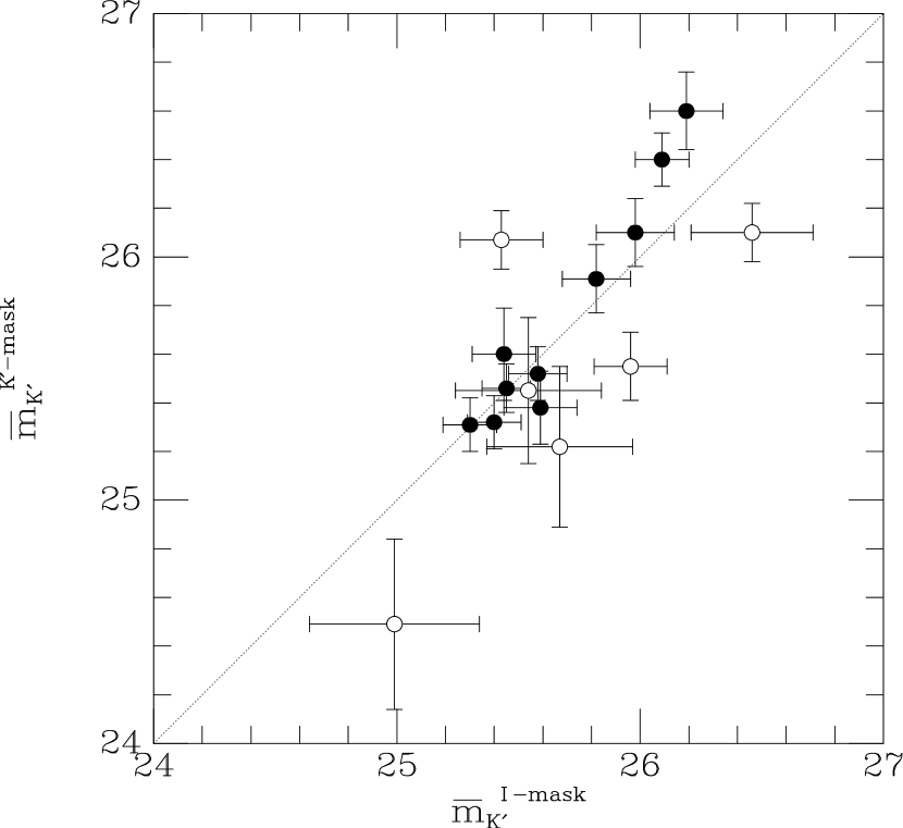
Figure 5: Comparison of fluctuation magnitudes $\overline{m}_{K^{\prime}}$ using $I$ and ${K^{\prime}}$ globular cluster and galaxy masks. The dotted line passes through the origin and has a slope of 1, and is not a fit to the data. Low-$S/N$ ratio points are plotted with open symbols. The error bars on the ${K^{\prime}}$-mask data are incomplete because no residual variance corrections were made for these measurements.

Fluctuation magnitudes were also measured for the four ellipticals in the Eridanus cluster, following the same procedures as those used to measure SBFs in the Fornax galaxies (Tables 3 and 4). Because the Fornax observations were our first priority, somewhat less time was allocated to the Eridanus galaxies. Eridanus is also more distant, so the resulting observations have significantly lower in their $S/N$ ratios. Only NGC 1407 has a ratio of ${P_{0}/P_{1}}\,{>}\,3$.

Estimating uncertainties for $\overline{m}_{K^{\prime}}$ can be difficult. We proceeded by first identifying all the probable sources of error: the statistical uncertainty in the fit for $P_{0}$, errors in measuring the sky offset, errors in fitting the galaxy profile, uncertainties in subtracting sources of residual variance, and so forth. We modified the parameters individually through their full ranges and measured the change in $P_{0}$. From the change in $P_{0}$ we estimated the 1-$\sigma$ uncertainty arising from the parameter in question. We then combined the uncertainties in quadrature to get the uncertainties listed in Tables 3 and 4. This procedure assumes that the different sources of uncertainty are independent, an assumption which is not strictly true. For example, modifying the residual sky level affects the fit to the galaxy profile slightly. Errors in fitting the galaxy profile affect our estimate of residual spatial variance as well. In the procedure used to fit the luminosity functions of the globular clusters and background galaxies, an error in one component obviously affects the fit to the other. While the cross correlations are obviously not zero, they were found to be small compared to the principal errors. The uncertainties computed are reasonable when we compare them with other distance estimates to calibrate the ${K^{\prime}}$ SBF distance scale.

4.2 Virgo Revisited

We reanalyzed the data originally presented by JLT using the updated SBF techniques presented in this paper. We improved our ${K^{\prime}}$ SBF measurements by determining the globular cluster and background galaxy contributions to the fluctuation amplitude. We also calculated magnitudes using the masks generated from the $I$-band images and applied a residual variance correction, just as we did for the Fornax and Eridanus galaxies. New fluctuation magnitudes are listed in Tables 3 and 4. Observations of five Virgo cluster galaxies are higher in $S/N$ ratio than the Fornax and Eridanus data, and it is reassuring to find that the GC, galaxy, and residual pattern corrections are quite small. The difference between fluctuation magnitudes measured using the different masks is negligible. In the NICMOS data, the field of view was small enough that very few GCs were observed, and the SBF $S/N$ ratio was high enough that the GC contribution was negligible.

Three of the Virgo galaxies had low $S/N$ ratios, two of which appeared to have anomalously bright fluctuations (JLT, Pahre & Mould 1994). In our reanalysis of the JLT Virgo data, NGC 4578 was found to have a $\overline{m}_{K^{\prime}}$ typical for the Virgo cluster but a large uncertainty due to the low $S/N$ ratio. The fluctuation magnitudes reported for NGC 4365 by JLT and Pahre & Mould (1994) were anomalously bright, if this galaxy resides in the Virgo W cloud behind the main Virgo cluster core (Tonry et al. 1990, Forbes 1996). We re-observed this galaxy in 1996 using the science-grade HAWAII detector and applied the full corrections for the globular cluster and background galaxy contributions. The new observations confirmed that the earlier measurement was biased by a significant GC population masquerading as stellar SBFs. Applying the GC correction to the 1995 data (JLT) brought it into agreement with the 1996 observation reported here. Applying the $I$-band GC mask allowed us to further check the consistency of the ${K^{\prime}}$ measurement. Magnitudes listed in Tables 3 and 4 are for the new 1996 data. When we used the $I$-band mask to remove GCs from the ${K^{\prime}}$ image, we measured a fluctuation magnitude of ${\overline{m}_{K^{\prime}}}\,{=}\,26.09\,{\pm}\,0.11$ mag. NGC 4365 illustrates that SBF amplitudes can be too large, making the galaxy appear significantly closer than it really is, if exposure times are not long enough to achieve a sufficiently high $S/N$ ratio and the globular cluster contribution is not adequately measured. With no a priori knowledge of the distance to NGC 4365 and follow-up observations, the JLT data would have lead to the incorrect conclusion that this galaxy resides in the main Virgo cluster.

JLT and Pahre & Mould (1994) also observed an anomalously bright fluctuation magnitude in NGC 4489. We have not yet re-observed this galaxy, and reanalysis of the JLT data does not expose an obvious GC contribution that could be responsible for the fluctuation magnitude measured.

4.3 The Effect of Low ${\bf S/N}$ Ratios on IR SBF Measurements

We have referred to $P_{0}/P_{1}$ as the $S/N$ ratio. With a better understanding of the variance arising from sources other than the stellar SBFs, we computed a more realistic measure of the $S/N$ ratio:

$${\xi}={{(P_{0}-P_{r}-P_{g})}\over{(P_{1}+P_{g})}}$$ (14)

Values for $\xi$ are listed in Table 4. Galaxies for which ${\xi}\,{<}\,1$ were not included in the calibration of $\overline{M}_{K^{\prime}}$. Comparison of the fluctuation magnitudes listed in Tables 3 and 4 showed that the SBF magnitudes for these low-$S/N$ ratio galaxies are unreliable, in agreement with the conclusion reached by JLT from analysis of the Virgo data alone. The differences are plotted as a function of $\log({\xi})$ in Figure 6. The mean difference between $\overline{m}_{K^{\prime}}$ values for the low-$S/N$ ratio observations is 0.41 mag; for the galaxies with ${\xi}\,{>}\,1$ the difference is only 0.15 mag, comparable to the individual uncertainties. The highest-$S/N$ ratio observations show the smallest difference between values of $\overline{m}_{K^{\prime}}$ measured with and without the $I$-band point-source masks. It is clear that when either $P_{r}$ or $P_{g}$ exceeds ${\sim}0.3P_{0}$, the resulting $\overline{m}_{K^{\prime}}$ is unreliable. In the following section, only the observations with ${\xi}\,{>}\,1$ (or ${P_{0}/P_{1}}\,{\gtrsim}\,3$) were included in the statistical analysis. From our observations we conclude that it is crucial that future IR SBF observations be deep enough to ensure that all sources of variance can be removed and that the $S/N$ ratio of the stellar SBFs is larger than 1.

The definition of $\xi$ in Equation 14 is empirical, but we can also use the results of our survey to predict $\xi$ as a function of observational parameters. The relationship can be approximated as

$${\xi}\approx 0.4\,D\,\theta^{-1/2}\,\left({{1000~{}{{\rm km\,s}^{-1}}}\over{cz}}\right)\left({{t_{exp}}\over{1000~{}{\rm s}}}\right)^{1/2}$$ (15)

where $D$ is the telescope diameter in meters and $\theta$ is the seeing FWHM in arcseconds. The relationship between $\xi$ and the observational parameters is not particularly good because a number of other parameters also affect the measured value of $\xi$. Equation 15 provides a basic guideline for the minimum integration required to make $K$-band SBF measurements. The coefficient in Equation 15 is somewhat less than the value of 0.5 found by Pahre & Mould (1994), and we emphasize that achieving a ${\xi}\,{=}\,1$ is marginal and assumes that residual variances have been subtracted. To make reliable $K$-band SBF distance measurements, we recommend that on-source integration times be

$$t_{exp}>6\,D^{-2}\,\theta\,\left({{cz}\over{1000~{}{{\rm km\,s}^{-1}}}}\right)^{2}\,\times 1000~{}{\rm s}.$$ (16)

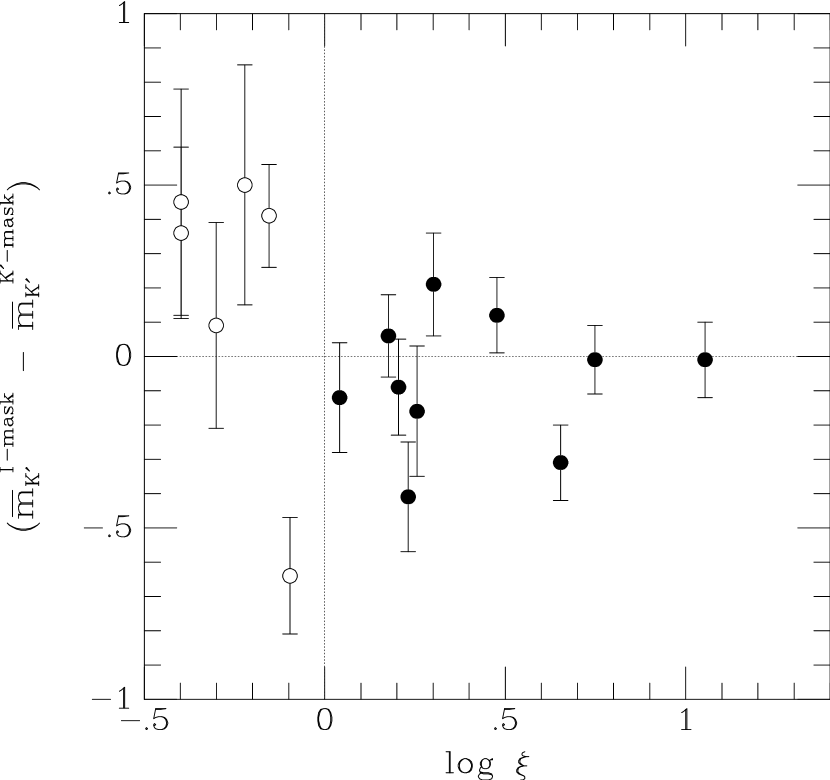
Figure 6: The differences between fluctuation magnitudes $\overline{m}_{K^{\prime}}$ measured using the $I$ and ${K^{\prime}}$ globular cluster masks are plotted as a function of log($\xi$). We plot the logarithm of the $S/N$ ratio because $\overline{m}_{K^{\prime}}$ is proportional to log($P_{0}$) and $\xi$ is proportional to $P_{0}$. Low-$S/N$ ratio measurements show the greatest differences between measurements using different masks. Measurements with ${\xi}\,{<}\,1$ (open symbols to the left of the vertical line) were not included in the calibration of $\overline{M}_{K^{\prime}}$.

5 The ${K^{\prime}}$ SBF Distance Scale Calibration

5.1 Adopted Distances

To calibrate the ${K^{\prime}}$ SBF distance scale, we first calculated absolute fluctuation magnitudes $\overline{M}_{K^{\prime}}$ for the high-$S/N$ ratio galaxies in our sample. We adopted three different (but not independent) sets of distances: Cepheid distances to M31 and the Virgo cluster, $I$-band SBF distances to individual galaxies, and cluster $I$-band SBF distances averaged over a larger sample of galaxies than we observed at ${K^{\prime}}$.

Our calibration of the IR SBF distance scale is strengthened significantly by the Cepheid distances to several Virgo spirals that have now been measured (Freedman et al. 1994; Pierce et al. 1994; Ferrarese et al. 1996; Saha et al. 1996a,b; Sandage et al. 1996). Of the five reported Cepheid distance measurements, four were made using data acquired using the Hubble Space Telescope. Three of these HST measurements are remarkably consistent: NGC 4321 $(m{-}M)\,{=}\,31.04\,{\pm}\,0.17$ (Ferrarese et al. 1996), NGC 4496a $(m{-}M)\,{=}\,31.03\,{\pm}\,0.14$ (Saha et al. 1996b), NGC 4536 $(m{-}M)\,{=}\,31.10\,{\pm}\,0.13$ (Saha et al. 1996a); NGC 4639 is ${\sim}1$ mag more distant than the other Virgo Cepheid distances (Sandage et al. 1996). Like NGC 4365, it is probably a member of the background Virgo W cloud, and has been excluded from the average Virgo Cepheid distance modulus used to calibrate the ${K^{\prime}}$ SBF distance scale. We adopt a cluster distance of $(m{-}M)\,{=}\,31.06\,{\pm}\,0.13$ ($d\,{=}\,16.27$ Mpc) for the Virgo cluster.

Recently the HST Key Project Team has measured a Cepheid distance to the Fornax spiral galaxy NGC 1365. At this time the analysis is nearly complete, and the Cepheid distance modulus to NGC 1365 is approximately $(m{-}M)\,{=}\,31.30$ (Silbermann 1998). In the near future HST Cepheid distances to three Fornax cluster galaxies will be measured by the Key Project team. Until then, we use only the Cepheid distances to M31 and the Virgo cluster to calibrate the ${K^{\prime}}$ SBF distance scale.

J. Tonry and collaborators are in the process of publishing the results of an extensive $I$-band SBF survey (Tonry et al. 1997). The $I$-band SBF distance scale was calibrated using Cepheid distances to a number of galaxies out to 20 Mpc. We can use $I$-band distances to calibrate the ${K^{\prime}}$ SBF scale using a larger sample of galaxies than using the ${K^{\prime}}$ SBF and Cepheid distances alone. We used the $I$-band data in two ways. First, distances to individual galaxies (Tonry 1997) gave absolute fluctuation magnitudes directly for each galaxy. Second, mean distances to each cluster (Tonry et al. 1997) were used, allowing us to take advantage of a larger sample but requiring us to assume that all the galaxies in a cluster are at the same distance. In both cases the $I$-band distances were calculated according to the calibration of Tonry et al. (1997). $I$-band distance moduli are listed in Table 8.

Recent measurements by the Hipparcos astrometric satellite have suggested that a systematic error in the Cepheid distance scale may exist because of an error in the parallax distances to the nearest stars (Feast & Catchpole 1997). If this is the case, all Cepheid distances need to be increased by ${\sim}10\%$, although the exact change may depend on metallicity corrections to the period-luminosity relation for Cepheid variables (Madore & Freedman 1997). The Cepheid zero-point correction also affects the $I$-band SBF distances, since they are also calibrated using the Cepheid distance scale. Because this issue has not yet been resolved, we adopt the distances cited above with a caution to the reader that the ${K^{\prime}}$ SBF distance calibration presented in this paper may need to be revised in the future.

5.2 Theoretical Stellar Populations

Surface brightness fluctuations can also be calibrated using theoretical models by computing the second moment of the luminosity function for a stellar population and normalizing by the first moment. If we know the absolute magnitudes of the brightest stars (which dominate the second moment of the luminosity function) from stellar population models, we can determine the distance directly from the apparent SBF magnitude. Alternatively, we can check our empirical calibration of the SBF distance scale against the synthesized stellar population models. G. Worthey produced a set of single-age, single-metallicity stellar population models and computed fluctuation magnitudes in the Johnson $J$, $H$, and $K$ bands (Worthey 1994, 1993b). He kindly created new models specifically for the ${K^{\prime}}$ filter, and we compare our fluctuation magnitudes with these new models (Worthey 1997). The ${K^{\prime}}$ SBF models show only slight differences from the $K$ models, but are significantly different from the $K$ models transformed to ${K^{\prime}}$ using the standard relation from Wainscoat & Cowie (1992). SBFs are considerably redder than the stars upon which the Wainscoat & Cowie transformation is based. The new ${K^{\prime}}$ model magnitudes are listed in Table 5. The fact that the new ${K^{\prime}}$ models are similar to the $K$ models is reassuring. The detailed stellar population models Worthey created include the CO absorption bandhead, which falls close to the edge of the $K$ window. We were not certain to what extent differences in CO absorption between the $K$ and ${K^{\prime}}$ filters would affect the measured SBF magnitudes. Now that Worthey (1997) has produced models precisely for our filter, we can compare them to our observations with confidence. The relatively small difference (${\lesssim}0.03$ mag) between $K$ and ${K^{\prime}}$ SBF magnitudes allows us to compare to Pahre & Mould (1994, $K_{\rm sh}$) as well since $K_{\rm sh}$ is centered midway between $K$ and ${K^{\prime}}$. We make a detailed comparison of our data with Worthey’s models in the following section.

Table 5: ${K^{\prime}}$ Fluctuation Magnitudes from Stellar Population Models

Age (Gyr)	[Fe/H]	Mg2	$(V{-}I)$	$\overline{M}_{K^{\prime}}$
5	$-0.22$	0.185	1.121	$-5.75$
	$0.00$	0.215	1.186	$-5.83$
	$0.25$	0.268	1.291	$-5.78$
	$0.50$	0.316	1.355	$-5.98$
8	$-2.00$	0.034	0.800	$-3.90$
	$-1.50$	0.056	0.846	$-4.11$
	$-1.00$	0.092	0.887	$-4.47$
	$-0.50$	0.160	1.083	$-5.13$
	$-0.25$	0.194	1.147	$-5.66$
	$0.00$	0.239	1.258	$-5.73$
	$0.25$	0.290	1.346	$-5.75$
	$0.50$	0.331	1.395	$-5.94$
12	$-2.00$	0.042	0.857	$-3.81$
	$-1.50$	0.064	0.892	$-4.03$
	$-1.00$	0.100	0.930	$-4.38$
	$-0.50$	0.171	1.110	$-5.08$
	$-0.25$	0.214	1.204	$-5.55$
	$0.00$	0.258	1.304	$-5.70$
	$0.25$	0.314	1.396	$-5.76$
	$0.50$	0.350	1.427	$-5.96$
17	$-2.00$	0.046	0.897	$-3.78$
	$-1.50$	0.069	0.937	$-4.15$
	$-1.00$	0.115	0.975	$-4.47$
	$-0.50$	0.187	1.159	$-5.08$
	$-0.25$	0.231	1.247	$-5.47$
	$0.00$	0.275	1.342	$-5.64$
	$0.25$	0.335	1.444	$-5.76$
	$0.50$	0.374	1.482	$-5.95$

In addition to single-age, single-metallicity populations, we also considered simple composite populations. We used Worthey’s (1994) $K$-band models to show that models vary smoothly between grid points. We tried combining a (8, $-0.25$) (Gyr, [Fe/H]) population with a (17, $-0.5$) population, with the younger population weighted by 5% to 50% (by mass). The point in $\overline{M}_{K}$ halfway between the two models was reached when 30% of the population was younger. We also combined a (12, $-0.25$) model with a (5, 0.0) stellar population and found the midpoint to be at the same ratio of populations. In other words, at least 30% of the stellar population by mass must be young for the young stars to dominate the $K$-band SBF magnitude. An old population will not look like a significantly younger population in $K$-band fluctuation magnitude if only a few percent of the mass is in the young population. Stellar populations younger than 5 Gyr were not considered. Because fluctuations are dominated by the brightest stars in the population, model SBF magnitudes are sensitive to the treatment of the complex stellar physics of the luminous asymptotic giant branch (AGB) stars. Fluctuations significantly brighter than model predictions may be evidence for young populations with brighter AGB stars than the model population.

G. Worthey’s models (1997) also predict the redshift dependence of the SBF magnitudes as a function of age. In Table 6 we list the K corrections in the $K$ band for redshifts between $0\,{\leq}\,z\,{\leq}\,0.03$. The models are all for solar metallicity [Fe/H] = 0. The tabulated values must be added to apparent $K$-band SBF magnitudes to find the equivalent magnitude at $z\,{=}\,0$. The K corrections for $K$-band SBFs are very small, especially for the older stellar populations. For the galaxies in this study, K corrections can be ignored. Even in future $K$-band SBF observations out to 10,000 km s^-1, uncertainties due to K corrections will be negligible.

Table 6: $K$-band SBF K corrections

$z$	5 Gyr	8 Gyr	12 Gyr	17 Gyr
0.005	0.004	0.003	0.002	$-0.001$
0.010	0.008	0.006	0.003	$-0.003$
0.015	0.011	0.008	0.003	$-0.005$
0.020	0.013	0.010	0.003	$-0.008$
0.025	0.015	0.012	0.003	$-0.011$
0.030	0.017	0.013	0.002	$-0.015$

5.3 Disentangling the Effects of Age and Metallicity

5.3.1 Fluctuation Magnitudes and $(V{-}I)$ Color

Broad-band colors are frequently used to constrain the properties of stellar populations. In the optical $I$ band, the effects of age and metallicity on SBFs are degenerate. Therefore the $I$-band SBF distance scale can be calibrated using the $(V{-}I)$ color to parameterize both the age and metallicity of stellar populations (Tonry 1997, Worthey 1993a). $I$-band SBFs are sensitive to galaxy color and $\overline{M}_{I}$ has a fairly steep slope with $(V{-}I)$, but the scatter is small and $I$-band SBFs can be used to measure accurate distances over a wide range of stellar population. At ${K^{\prime}}$, stellar population models (Worthey 1993a, 1997) predict a shallower slope with $(V{-}I)$, but more importantly, the slope is opposite in sign. Age and metallicity effects do not counteract each other as in the $I$-band. Because the age-metallicity degeneracy is partially broken, the dispersion in fluctuation magnitudes is also expected to be larger than at $I$. To explore the behavior of ${K^{\prime}}$ SBFs with $(V{-}I)$ color, we plotted the fluctuation magnitudes $\overline{m}_{K^{\prime}}$ as a function of $(V{-}I)$ in Figure 7. Filled circles denote those measurements for which the $S/N$ ratio was large (${\xi}\,{>}\,1$ or ${P_{0}/P_{1}}{\geq}2.8$). The $\overline{m}_{K^{\prime}}$ magnitudes derived using the $I$-band masks were used to create the figures in this section. We superimposed Worthey’s ${K^{\prime}}$ models (1997), with grid lines labeled by age and metallicity. To place the models, we used the mean Cepheid distance for Virgo and cluster $I$-band SBF distances for the Fornax and Eridanus clusters.

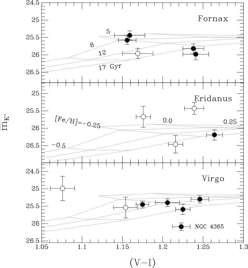
Figure 7: Apparent fluctuation magnitudes $\overline{m}_{K^{\prime}}$ are plotted as a function of $(V{-}I)$ color for three clusters. Low-$S/N$ ratio measurements are indicated by open circles. ${K^{\prime}}$ stellar population models (Worthey 1997) are labeled according to age and metallicity. NGC 4365 resides in the W cloud, behind the main Virgo cluster core. The majority of the galaxies studied have fluctuation magnitudes consistent with older stellar populations (12 to 17 Gyr), but those with bluer optical colors show evidence of younger stellar populations. Low-$S/N$ ratio observations (open symbols) are unreliable.

From Figure 7 we learn that the galaxies on the red end of the sample are mostly consistent with older, 12 to 17 Gyr stellar populations with metallicities near [Fe/H] = $-0.25$. The bluer galaxies with ${(V{-}I)}\,{\approx}\,1.15$ have fluctuation magnitudes consistent with 5 to 8 Gyr population models and similar metallicities. The trend is easily seen in Figure 8, in which we plotted the absolute fluctuation magnitudes $\overline{M}_{K^{\prime}}$ as a function of $(V{-}I)$ for all the high-$S/N$ ratio observations in our sample. The upper panel in Figure 8 used the Cepheid distances to M31 and the Virgo galaxies; the lower panel was plotted using the $I$-band SBF distances to individual galaxies and includes galaxies in Fornax and Eridanus. For the bluer galaxies to be consistent with 12 to 17 Gyr population models, the SBF magnitudes would have to be at least 0.5 mag fainter. We see that the dispersion in $(V{-}I)$ color appears to be due to variations in population age, not metallicity. This conclusion contradicts the hypothesis that the dispersion in colors of elliptical galaxies is the result of metallicity variations (Buzzoni 1995). On the other hand, the age spread we infer from our data is consistent with the “bursty” formation scenario in which ellipticals form episodically, as predicted by the hypothesis that ellipticals form through mergers (Faber et al. 1995). Of course our sample is not very large, and this conclusion should be confirmed by additional high-$S/N$ ratio IR SBF measurements over a larger range of galaxy color.

Figure 8: Absolute fluctuation magnitudes $\overline{M}_{K^{\prime}}$ are plotted as a function of $(V{-}I)$ color, with the Worthey (1997) models superimposed. The top panel adopts the Cepheid distances to M31 and the Virgo cluster, while the bottom panel uses individual $I$-band SBF distance measurements from Tonry (1997) for all the high-$S/N$ ratio galaxies. Using the mean cluster $I$-band SBF distances from Tonry et al. (1997) changes the lower panel only slightly. The trend toward younger ages in the bluer galaxies is apparent, as is the obvious lack of a negative slope in $\overline{M}_{K^{\prime}}$ with increasing $(V{-}I)$ predicted by the models.

We also learn something from the galaxies whose fluctuation magnitudes are not consistent with the stellar population models shown. JLT and Pahre & Mould (1994) both noted two galaxies with anomalous ${K^{\prime}}$ SBF magnitudes in the Virgo cluster (NGC 4489 and NGC 4365). Our latest observations of NGC 4365 reveal that this galaxy is indeed in the background W cloud. The new fluctuation magnitude $\overline{m}_{K^{\prime}}$ is fully consistent with the $I$-band distance (Tonry 1997) and with the distance derived from the peak of the GCLF (Forbes 1996). As stated in Section 4.2 above, failure to remove significant residual variances (from globular clusters in this case) can result in significantly biased fluctuation measurements. NGC 4489’s low-$S/N$ ratio fluctuation magnitude $\overline{m}_{K^{\prime}}$ is ${\sim}1$ mag brighter than the model predictions. Either it is a young galaxy with a possibly anomalous AGB population, or the measurement is biased by residual variances which have not been adequately removed. NGC 4489 does not appear to have an extensive GC population as does NGC 4365, but it is unusual in other ways (JLT). Until deeper $K$-band images are obtained for NGC 4489, our conclusions regarding an anomalous stellar population will be uncertain. Observations of Fornax and Eridanus cluster galaxies have revealed other candidates with unusually bright ${K^{\prime}}$ SBF magnitudes; all have low $S/N$ ratios ${\xi}\,{<}\,1$. Comparison of the fluctuation magnitudes for NGC 1395 in Tables 3 and 4 reveals a difference of 0.64 mag. A reasonable correction for globular clusters from the ${K^{\prime}}$ observations brings the $\overline{m}_{K^{\prime}}$ into agreement with the stellar population models. Nevertheless, the $I$-band mask should remove the GCs much better than using the ${K^{\prime}}$ data alone. NGC 1426 is also seen to be anomalously bright in both Tables 3 and 4. Given that these observations all have low $S/N$ ratios, all appear too bright, and all have large (and uncertain) corrections for residual variances $P_{r}$ and $P_{g}$, we cannot draw any conclusions regarding their stellar populations. When ${\xi}\,{<}\,1$, fluctuation magnitudes are unreliable and are not included in the calibration of $\overline{M}_{K^{\prime}}$.

The high-$S/N$ ratio data plotted in Figure 8 can be fitted to find the relationship between $\overline{M}_{K^{\prime}}$ and $(V{-}I)$. The fits were performed using the three distance estimates and the two different sets of $\overline{m}_{K^{\prime}}$ values described in Sections 4.1 and 5.1 above. We used an iterative least-squares approach to weight each point according to the uncertainties in both $\overline{m}_{K^{\prime}}$ and $(V{-}I)$. The results are listed in Table 7, which includes the number of points used in the fit and $\chi^{2}$ per degree of freedom. The $I$-band GC masks produce calibrations of $\overline{M}_{K^{\prime}}$ with consistent zero points. Whether we use the individual $I$-band SBF distances or the mean distances for the clusters makes little difference. Somewhat greater scatter is observed in the zero points of the fits which use the ${K^{\prime}}$-mask data, confirming that the $I$-band GC and galaxy masks produce more consistent fluctuation magnitudes. The $\chi^{2}$ values indicate that our uncertainties are reasonable. The Cepheid fits include only 5 points, and we believe it is small number statistics, rather than overestimated errors, that causes $\chi^{2}/(n{-}2)\,{<}\,1$. Using the $I$-band SBF distances results in larger numbers of galaxies in the fits. Differences in age and metallicity between the galaxies produce a dispersion in $\overline{M}_{K^{\prime}}$ somewhat larger than our uncertainties, and the $\chi^{2}$ per degree of freedom is larger than one. The only statistically significant slopes we measured resulted from using the ${K^{\prime}}$ GC masks and the $I$-band SBF distances. The positive slope suggests that ${K^{\prime}}$ SBFs are fainter in redder galaxies, opposite the trend predicted by the stellar population models (Figure 8). No significant slope is seen in the data using the Cepheid distances alone, but only 5 points were included in this fit, so the lack of a correlation is not conclusive either. On the other hand, there is no convincing reason that a slope opposite that predicted by the models should exist. Our best ${K^{\prime}}$ SBF results are produced using the $I$-band masks, and the fits to these data are most consistent with a constant $\overline{M}_{K^{\prime}}$ across the range in $(V{-}I)$ spanned by our sample. This is a very useful feature, since it implies that accurate $(V{-}I)$ colors do not need to be measured to determine ${K^{\prime}}$ SBF distances. Future observations of a significantly larger sample including bluer galaxies will be required to determine whether or not ${K^{\prime}}$ SBFs get fainter as galaxies get bluer, as predicted by the stellar population models.

Table 7: Fits: ${\overline{M}_{K^{\prime}}}=a+b[{(V{-}I)}-1.2]$

Distances	Mask	$a$	$\pm$	$b$	$\pm$	$\chi^{2}/(n{-}2)$	$n$
Cepheids	$I$	$-5.61$	0.06	$-0.9$	1.8	0.8	5
$I$ SBF individual		$-5.61$	0.04	1.4	1.1	1.9	11
$I$ SBF group		$-5.55$	0.04	1.7	1.1	1.2	9
Cepheids	${K^{\prime}}$	$-5.65$	0.06	$-0.8$	1.8	0.6	5
$I$ SBF individual		$-5.56$	0.04	3.0	1.2	1.0	10
$I$ SBF group		$-5.53$	0.05	3.0	1.2	2.0	9

The $I$-band masks produce the most reliable fluctuation magnitudes, and the $I$-band SBF and Cepheid distance scale calibrations are equally good. We therefore adopt as the calibration of the ${K^{\prime}}$ SBF distance scale

$${\overline{M}_{K^{\prime}}}=-5.61\pm 0.12$$ (17)

with no $(V{-}I)$ term for the limited range $1.15\,{<}\,{(V{-}I)}\,{<}\,1.27$. The statistical uncertainty is 0.06 mag; adding 0.10 mag in quadrature for the Cepheid zero point uncertainty results in a total uncertainty of 0.12 mag. The statistical uncertainty in the zero point was derived by fitting a slope to $(V{-}I)$. The scatter due to variations in stellar population results in somewhat greater uncertainties when no correction for $(V{-}I)$ is made. Our calibration is consistent with the JLT measurement, which is not surprising given that the same Virgo data were used in both studies. This value for $\overline{M}_{K^{\prime}}$ is the same as that measured by Luppino & Tonry (1993) for M31, and is somewhat fainter than Pahre & Mould’s (1994) measurement of $M_{K_{sh}}\,{=}\,{-}5.77\,{\pm}\,0.18$, although the values are well within the errors. Our calibration was used to compute distance moduli for the galaxies in our survey, and we list distances in Table 8 with the $I$-band SBF distance moduli for comparison. The comparison between $I$ and ${K^{\prime}}$ distance moduli is presented graphically in Figure 9. The line shown is not a fit to the data, but simply the line with a slope of 1 which passes through the origin. The high-$S/N$ measurements are consistent with the $I$-band SBF distances. The errors listed for ${K^{\prime}}$ distance moduli are the individual errors in $\overline{m}_{K^{\prime}}$, and do not include the zero-point uncertainty. Mean ${K^{\prime}}$ SBF distances for each cluster are included with their standard deviations, where only the high-$S/N$ measurements were included in the mean. Once again, we note that since the same Cepheid calibration was used for all distances tabulated, a systematic change in the Cepheid distance scale will affect the $I$ and ${K^{\prime}}$ SBF distances equally.

Table 8: Comparison of Measured Distances

Galaxy	$(V{-}I)$	$\pm$	Mg2	$(m{-}M)_{\rm Ceph}$	${(\overline{m}{-}\overline{M})}_{I}$	$\pm$	${(\overline{m}{-}\overline{M})}_{{K^{\prime}}}$	$\pm$
Fornax				31.30	31.22	0.06	31.32	0.24
NGC 1339	1.169	0.019	0.328	$\cdots$	31.34	0.14	31.57	0.15
NGC 1344	1.156	0.011	0.290	$\cdots$	31.17	0.09	31.19	0.12
NGC 1379	1.159	0.019	0.284	$\cdots$	31.30	0.08	31.05	0.13
NGC 1399	1.241	0.016	0.361	$\cdots$	31.42	0.14	31.59	0.16
NGC 1404	1.238	0.013	0.344	$\cdots$	31.27	0.08	31.43	0.14
Eridanus				$\cdots$	31.71	$\cdots$	31.80	$\cdots$
NGC 1395	1.239	0.012	0.340	$\cdots$	31.63	0.41	31.04	0.17
NGC 1400	1.216	0.009	0.336	$\cdots$	31.67	0.14	32.07	0.25
NGC 1407	1.264	0.010	0.354	$\cdots$	32.02	0.19	31.80	0.15
NGC 1426	1.176	0.009	0.303	$\cdots$	31.80	0.08	31.28	0.30
Virgo				$31.06\pm 0.13$	30.96	0.05	31.06	0.12
NGC 4365	1.223	0.011	0.348	$\cdots$	31.70	0.09	31.70	0.11
NGC 4406	1.175	0.008	0.336	$\cdots$	31.19	0.07	31.06	0.10
NGC 4472	1.246	0.011	0.345	$\cdots$	30.94	0.06	30.91	0.11
NGC 4489	1.076	0.015	0.222	$\cdots$	$\cdots$	$\cdots$	30.60	0.35
NGC 4552	1.206	0.015	0.352	$\cdots$	30.86	0.08	31.05	0.11
NGC 4578	1.154	0.015	0.312	$\cdots$	31.25	0.08	31.15	0.30
NGC 4636	1.225	0.009	0.341	$\cdots$	30.83	0.08	31.20	0.15
Local Group
M31	1.240	0.007	0.334	$24.43\pm 0.10$	24.38	0.05	24.43	0.14
M32	1.145	0.007	0.199	$\cdots$	24.48	0.05	24.17	0.14

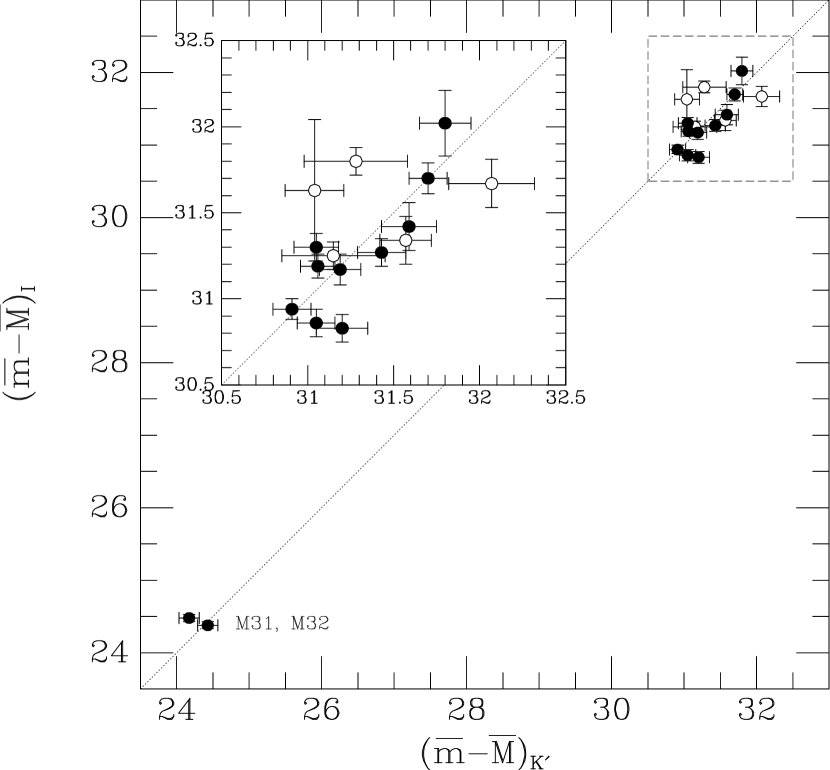
Figure 9: We plotted the $I$ and ${K^{\prime}}$ SBF distance moduli against each other to demonstrate the reliability of our high-$S/N$ measurements. The dotted line has a slope of 1 and passes through the origin; it is not a fit to the data. The Virgo, Fornax, and Eridanus cluster data are shown on an expanded scale in the inset box. Local Group measurements are taken from Luppino & Tonry (1993).

5.3.2 Fluctuation Magnitudes and Mg₂ Index

We also compared our ${K^{\prime}}$ fluctuation magnitudes with Worthey’s (1997) models as as function of the Mg₂ spectral index. Values of the Mg₂ index were taken from Faber et al. (1989), Worthey et al. (1992), and Worthey (1993a). There is a systematic offset between the Faber et al. and the Worthey et al. measurements, the latter being larger by about 8%. Seven galaxies in our sample have Mg₂ values listed by both Worthey et al. and by Faber et al. The offset of 0.027 mag between the two studies was used to adjust the Faber et al. data to the Worthey system for the Fornax and Eridanus cluster galaxies. Thus we compare the Worthey (1997) models with the most compatible Mg₂ data. Mg₂ values are listed in Table 8. We plotted $\overline{M}_{K^{\prime}}$ as a function of Mg₂ for the galaxies with ${\xi}\,{>}\,1$ in Figure 10 with the Worthey (1997) models superimposed, as in the previous section.

Figure 10: Absolute SBF magnitudes $\overline{M}_{K^{\prime}}$ are plotted versus the Mg₂ index. Simple stellar population models (Worthey 1997) are shown with age and metallicity grid lines labeled. The observations do not agree with the stellar population models, so we cannot use the Mg₂ index in conjunction with ${K^{\prime}}$ SBF magnitudes to better understand stellar populations within the context of the population models.

Very few of the observations fall within the range spanned by the models. For our observations to be consistent with the results of the previous section, Mg₂ indices must be reduced by ${\sim}0.15$ mag. The reason for the discrepancy is not known, but may be the result of significantly enhanced [Mg/Fe] ratios (0.2 to 0.3 dex) observed in giant ellipticals compared to stars in the solar neighborhood with similar metallicities (Worthey et al. 1992, Worthey 1994). We do not fit $\overline{M}_{K^{\prime}}$ as a function of Mg₂ to calibrate the ${K^{\prime}}$ SBF distance scale because of the small range in Mg₂ spanned by our data and the inconsistency with the stellar population models.

5.3.3 Radial Gradients in SBFs

Radial gradients in ${K^{\prime}}$ fluctuation magnitudes potentially reveal changing ages and metallicities within the stellar population of a galaxy. Tonry (1991) showed that the color gradient in NGC 205 correlates with a change in the $I$-band fluctuation magnitude $\overline{m}_{I}$. A younger stellar population at the center of NGC 205 gives rise to brighter $I$-band fluctuations at smaller radii than in the redder outer regions. Sodemann & Thomsen (1995) discuss the implications of a radially increasing $I$-band fluctuation amplitude observed in NGC 3379, opposite the trend seen in NGC 205. At $I$ the effects of age and metallicity on $\overline{m}_{I}$ are largely degenerate, making it difficult to interpret radial changes in fluctuation magnitude. Older stellar populations have fainter $\overline{m}_{I}$ magnitudes, but populations with higher metallicity also have fainter $\overline{m}_{I}$ magnitudes, making it impossible to distinguish between old, metal-poor and young, metal-rich populations. At ${K^{\prime}}$, on the other hand, the degeneracy is partially broken. The Worthey models (1993b, 1997) predict that IR fluctuations should fade with increasing age and decreasing metallicity, allowing us to separate young, metal-rich and old, metal-poor populations. If an elliptical galaxy is formed by merging which triggers a burst of new star formation, we would expect the outer envelope of such a galaxy to be older and more metal-poor than the nuclear region (Faber et al. 1995). The brighter $I$-band fluctuation magnitudes observed in the outer regions of NGC 3379 may be consistent with this scenario if the change is $\overline{m}_{I}$ is principally due to a decrease in metallicity; in NGC 205 the change in $\overline{m}_{I}$ must be due to age differences between the populations. Pahre & Mould (1994) observed no radial gradient in the $K$-band fluctuation magnitude in NGC 3379, but a modest gradient may be hidden in the scatter of the individual measurements.

While the prospects for using IR SBFs to reveal radial gradients in stellar populations are good, the data presented here do not have a sufficiently high $S/N$ ratio to detect radial changes in fluctuation amplitude; the uncertainties due to background subtraction and estimated residual variance mask the modest changes in $\overline{m}_{K^{\prime}}$ that might result from differences in stellar populations within a galaxy. If the outer regions of an elliptical galaxy are older and more metal-poor than the center, the ${K^{\prime}}$ fluctuation amplitude will decrease with radius. In our data, uncorrected fluctuation amplitudes usually increase with radius, sometimes changing by a factor of two. Even if we could imagine a scenario that creates a galaxy with the older stars at the center, the variations in stellar population that would be required to explain such large changes in fluctuation amplitude are not plausible. Instead, we interpret the observed SBF gradients in our data to be indicators of residual variations in the sky background.

Using IR SBFs to reach definitive conclusions regarding stellar population gradients in nearby galaxies will require high-$S/N$ ratio data in which corrections for residual variance are negligible. Although we have not conclusively measured IR SBF gradients it should be emphasized that the breaking of the age and metallicity degeneracy potentially makes IR SBFs a powerful probe for distinguishing old, metal-poor populations from younger, metal-rich stars. For example, the range in $(V{-}I)$ in NGC 205 should give rise to a change in $\overline{m}_{K^{\prime}}$ of ${\sim}0.5$ mag, with $\overline{m}_{K^{\prime}}$ becoming fainter with radius. If an IR SBF gradient were detected in NGC 3379, we could explain the very different optical SBF properties of these two galaxies in terms of the ages and metallicities of the stellar populations.

6 Summary

We have completed a ${K^{\prime}}$ (2.1 µm) survey of surface brightness fluctuations in 16 giant elliptical galaxies in the Virgo, Fornax, and Eridanus clusters. We also observed M31 and M32 in the $J$ and $H$ bands. From this study we draw the following conclusions:

$K$-band SBFs can be measured reliably and used to determine distances to early-type galaxies. Because SBFs are relatively bright in the IR and the seeing is typically very good, integration times can be quite modest. However, observations must be sufficiently deep to adequately sample the GC luminosity function and remove sources of residual variance. Low-$S/N$ ratio measurements are unreliable. Optical images can be used to identify and remove GCs and background galaxies that are not detected in the IR, improving the IR SBF measurement. We empirically calibrated the ${K^{\prime}}$ SBF distance scale using Cepheid distances to M31 and the Virgo cluster. The absolute ${K^{\prime}}$ fluctuation magnitude is ${\overline{M}_{K^{\prime}}}\,{=}\,{-}5.61\,{\pm}\,0.06$ (statistical error) with a total uncertainty of 0.12 mag. No significant change in $\overline{M}_{K^{\prime}}$ with $(V{-}I)$ was observed over the range in color spanned by the galaxies in this sample. Accurate color measurements are not required to measure the ${K^{\prime}}$ SBF distance to a galaxy.

${K^{\prime}}$ SBF magnitudes are consistent with predictions from simple stellar population models. The lack of a correlation in $\overline{M}_{K^{\prime}}$ with $(V{-}I)$ is best explained by a spread in ages among the galaxies observed. The redder ellipticals are consistent with 12 to 17 Gyr stellar population models, while the bluer galaxies in our sample must have younger 5 to 8 Gyr populations. Metallicities appear to vary less than ages, with the typical galaxy having [Fe/H] = ${-}0.25$. The stellar population models show that the age-metallicity degeneracy is broken with $K$-band SBFs, allowing one to distinguish between old, metal-poor and young, metal-rich populations. Examining the radial variation in IR SBFs will help distinguish between different galaxy formation scenarios. Our observations do not agree with the relationship between $\overline{M}_{K^{\prime}}$ and the Mg₂ index predicted by the stellar population models.

References

- (1) Ajhar, E. A. & Tonry, J. T. 1994, ApJ, 429, 557
- (2) Blakeslee, J. P. 1997, ApJ, 481, L59
- (3) Blakeslee, J. P. & Tonry, J. L. 1995, ApJ, 442, 579
- (4) Blakeslee, J. P. & Tonry, J. L. 1996, ApJ, 465, L19
- (5) Blakeslee, J. P., Tonry, J. L., & Metzger, M. R. 1997, AJ, 114, 482
- (6) Burstein, D. & Heiles, C. 1984, ApJS, 54, 33
- (7) Buzzoni, A. 1995, ApJS, 98, 69
- (8) Casali, M. & Hawarden, T. G. 1992, JCMT-UKIRT Newsletter, 4, 33
- (9) Cohen, J. G., Frogel J. A., Persson, S. E., & Elias, J. H. 1981, ApJ, 249, 481
- (10) Cowie, L. L., Gardner, J. P., Hu, E. M., Songaila, A., Hodapp, K.-W., & Wainscoat, R. J. 1994, ApJ, 434, 114
- (11) Djorgovski, S. et al., 1995, ApJ, 438, 13
- (12) Faber, S. M., Trager, S. C., Gonzalez, J. J., & Worthey, G. 1995, in Stellar Populations, I.A.U. Symp. 164, eds. P. C. van der Kruit & G. Gilmore (Kluwer, Dordrecht), p. 249
- (13) Faber, S. M., Wegner, G., Burstein, D., Davies, R. L., Dressler, A., Lynden-Bell, D., & Terlevich, R. J. 1989, ApJS, 69, 763
- (14) Feast, M. W. & Catchpole, R. M. 1997, MNRAS, 286, L1
- (15) Ferrarese, L. et al. 1996, ApJ, 464, 568
- (16) Forbes, D. 1996, AJ, 112, 954
- (17) Freedman, W. L. & Madore, B. F. 1990, ApJ, 365, 186
- (18) Freedman, W. L. et al. 1994, Nature, 371, 757
- (19) Frogel, J. A., Persson, S. E., Aaronson, M., & Matthews, K. 1978, ApJ, 220, 75
- (20) Glass, I. S. 1984, MNRAS, 211, 461
- (21) Hodapp, K.-W. et al. 1996, New Astronomy, 1, 177
- (22) Hodapp, K.-W., Rayner, J., & Irwin, E. 1992, PASP, 104, 441
- (23) Jacoby, G. H., Branch, D., Ciardullo, R., Davies, R. L., Harris, W. E., Pierce, M. J., Pritchet, C. J., Tonry, J. L., & Welch, D. L. 1992, PASP, 104, 599
- (24) Jensen, J. B., Luppino, G. A., & Tonry, J. L. 1996, ApJ, 468, 519 (JLT)
- (25) Luppino, G. A. & Tonry, J. L. 1993, ApJ, 410, 81
- (26) Madore, B. F. & Freedman, W. L. 1997, ApJ, 492, 110
- (27) Pahre, M. A. & Mould, J. R. 1994, ApJ, 433, 567
- (28) Persson, S. E., Cohen, J. G., Sellgren, K., Mould, J., & Frogel, J. A. 1980 ApJ, 240, 779
- (29) Persson, S. E., Frogel, J. A., & Aaronson, M. 1979, ApJS, 39, 61
- (30) Pierce, M. J., Welch, D. L., McClure, R. D., van den Bergh, S., Racine, R., & Stetson, P. B. 1994, Nature, 371, 385
- (31) Saha, A., Sandage, A., Labhardt, L, Tammann, G. A., Macchetto, F. D., & Panagia, N. 1996a, ApJ, 466, 55
- (32) Saha, A., Sandage, A., Labhardt, L, Tammann, G. A., Macchetto, F. D., & Panagia, N. 1996b, ApJS, 107, 693
- (33) Sandage, A., Saha, A., Tammann, G. A., Labhardt, L., Panagia, N., & Macchetto, F. D. 1996, ApJ, 460, L15
- (34) Schechter, P. L., Mateo, M., & Saha, A. 1993, PASP, 105, 1342
- (35) Secker, J. & Harris, W. E. 1993, AJ, 105, 1358
- (36) Silbermann, N. 1998, private communication
- (37) Sodemann, M. & Thomsen, B. 1995, AJ, 110, 179
- (38) Sodemann, M. & Thomsen, B. 1996, AJ, 111, 208
- (39) Tonry, J. L. 1991, ApJ, 373, L1
- (40) Tonry, J. L. 1997, private communication
- (41) Tonry, J. L., Ajhar, E. A., & Luppino, G. A. 1990, AJ, 100, 1416
- (42) Tonry, J. L., Blakeslee, J. P., Ajhar, E. A., & Dressler, A. 1997, ApJ, 475, 399
- (43) Tonry, J. L. & Schneider, D. P. 1988, AJ, 96, 807
- (44) Wainscoat, R., Cohen, M., Volk, K., Walker, H. J., & Schwartz, D. E. 1992, ApJS, 83, 111
- (45) Wainscoat, R. & Cowie, L. 1992, AJ, 101, 332
- (46) Worthey, G. 1993a, ApJ, 409, 530
- (47) Worthey, G. 1993b, ApJ, 418, 947
- (48) Worthey, G. 1994, ApJS, 95, 107
- (49) Worthey, G. 1997, private communication
- (50) Worthey, G., Faber, S. M., & Gonzalez, J. J. 1992, ApJ, 398, 69