Turbulent Convective Cepheid Models: Linear Properties

Abstract

A one-dimensional turbulent convection model in the form of a time-dependent diffusion equation for the turbulent energy is incorporated into our numerical pulsation code. The effect of turbulent convection on the structural rearrangement of the static equilibrium star is taken into account, and the linear eigenvalues (periods and growth-rates) for the complete turbulent convective nonadiabatic pulsations of the equilibrium models are calculated. The linearized code allows us to perform efficiently a systematic survey of the stability of Cepheid models for a wide range of astrophysical parameters ($L$,$M$,$T_{ef\!f}$) and the turbulent convective parameters.

A sensitivity analysis of the properties of several sequences of Galactic Cepheids is performed with the goal of using observational constraints, such as the shape and location of the fundamental and first overtone instability strips, to calibrate the turbulent convective input parameters. The locations of the red and blue edges of the fundamental and first overtone instability strips and the overall strip widths are largely determined by the parameters that determine the mixing length, and strengths of the eddy viscosity and of the convective flux. The remaining parameters can be used for fine-tuning agreement with observations.

1 Introduction

Cepheid studies have acknowledged, right from the beginning, that convection should occur in Cepheid envelopes, and that they should alter the properties of both the pulsations and the underlying equilibrium models. Since the Prandtl number characteristic of stellar material is very small, ${P\negthinspace{\scriptstyle r}}\sim O(10^{-9})$, and the Rayleigh numbers associated with the partial ionization regions (PIR) are enormous, ${R{\scriptstyle a}}$  $>$$\sim$  $O(10^{12})$, stellar convection is far into the hard turbulent regime (Krishnamurti & Howard Ruby (1983)). The cooler Cepheid stars are believed to have the more extensive convection zones, leading to pulsational stability beyond the red edge of the standard instability strip (IS). Because of the estimated inefficiency of convection and because of the difficulties of treating turbulent convection, a lot of work has disregarded it altogether, the hope having been that, except for providing a red edge, convection would play a subdued role. And purely radiative models have indeed provided a reasonable overall agreement with observations.

More recently it has become increasingly clear that an impasse has been reached with radiative models, and that it is not possible to improve the agreement with observations (e.g. Buchler Buchler97 (1997)). In particular, the amplitudes of pulsation are systematically too large. No consistent set of pseudo-viscous parameters can correctly limit the amplitudes of both fundamental and first overtone pulsations without adversely affecting the stability of the corresponding limit cycles, and the agreement with observation. The new EROS and MACHO data of the low metallicity Magellanic Cloud Cepheids (Buchler et al. BKBG (1996)) reveals further disagreement between stellar evolution and radiative stellar pulsation models. Clearly some additional physical dissipation is missing in the radiative codes (see also Kovács Kovacs (1990)), and turbulence and convection are the primary suspects.

Simulation of even the simplest turbulent convection (TC) problem is a formidable numerical challenge; to adequately resolve the many time- and length-scales of fully turbulent 3D convection at stellar Rayleigh and Prandtl numbers is totally out of question, and astrophysicists have been looking for 1D recipes to give an approximate, but acceptable treatment of this phenomenon. Thus the 1925 mixing length picture of Prandtl was readily adapted to stellar envelopes by Böhm-Vitense, and subsequently reformulated in many variations, all of which are equivalent for time-independent problems (for an overview, see Baker Baker (1987)). But time-independent MLT was never able to resolve the red edge problem, mostly because it is time-dependent dissipation introduced by eddy viscosity that provides a clear red edge, as we will show in § 4.6. Spiegel Ed63 (1963) first extended MLT to the time-dependent and nonlocal cases. The earliest attempts to include a time-dependent mixing length model in pulsation (Gough Gough (1977), Unno Unno (1967)) were not successful because they were too local in space. Subsequently, Gough’s theory was extended to be less local, and eventually was used in a full linearization of Solar modes (Balmforth Neil (1992)), analogous to what we have done here. Unno’s theory was also developed (Castor Castor (1968)) as a diffusion model, and simplified to a single equation for the turbulent energy $e_{t}$ by Stellingwerf (Swf82 (1982)). More recent applications of this and similar turbulent diffusion recipes have been made by Gonczi & Osaki Gonc-O (1980), Bono & Stellingwerf BS (1994), Gehmeyr & Winkler Geh-W (1992), hereafter GW) and Kuhfuss (KuhfuB (1986)). Further closely related models also appear in the literature, such as those of Canuto (Canuto (1991)) but have yet to be applied.

All 1D model TC equations contain several dimensionless, order unity parameters that are directly related to the physical quantities of the model. In principle, the validity of the 1D model equation can be checked against experiments or against detailed 3D simulations of turbulent convection, and values of the unknown parameters can be extracted. However, neither such experiments nor such simulations are presently available. We are obliged to calibrate these parameters indirectly with the help of observational astronomical constraints, as suggested more than a decade ago by Stellingwerf (Swf82 (1982)). In the best outcome, observational constraints could select one model in favor of the others. On the other hand we might discover that single equation models for turbulent convection are insufficient, or that plumes (e.g. Rieutord & Zahn R-Zahn (1995)) play an essential role in the convective transport.

This programme has recently been initiated by incorporating these recipes into hydrodynamic pulsation codes. Fully nonlinear models have been used to determine the stability properties of convective pulsators (e.g. Bono & Stellingwerf BS (1994), Bono & Marconi BM97 (1997)), but this approach is inefficient, and unsuitable when a large number of models is required. The approach we follow in this paper is to compute the linear nonadiabatic properties directly by linearizing the hydrodynamic equations about the equilibrium model and by then computing the linear eigenvalues, a procedure which is relatively fast. This allows us to perform an extensive survey of the sensitivity to the TC parameters.

2 The Turbulent Convective (TC) Model Equations

We have adopted a TC model equation that consists of a single diffusion equation for the turbulent energy and that includes the effects of the turbulent stress, turbulent energy flux and turbulent energy production on the mean momentum and energy; our model is essentially that used by Gehmeyr (Geh92 (1992)). In the following, we reproduce our PDE’s for the purpose of notation and for completeness. In addition to $dr/dt=u$ we have the momentum equation, modified to include the effects of turbulent stress, that are cast here in the form of a turbulent pressure and an eddy pressure

$${du\over dt}=-4\pi r^{2}{\partial\over\partial m}\left(p+p_{t}+p_{\nu}\right)-{GM(r)\over r^{2}}\thinspace.$$ (1)

The pressure $p$ and specific energy $e$ represent the combined gas and radiation quantities. We use the specific internal energy equation in the form

$$c_{v}{dT\over dt}=-{\left(p+\Bigl{(}{\partial e\over\partial v}\Bigr{)}_{T}\right)}{\partial(r^{2}u)\over\partial m}\\ -{\partial\over\partial m}\left[r^{2}\left(F_{c}+F_{r}\right)\right]+{\cal C}\,.$$ (2)

The turbulent specific energy itself satisfies a diffusion equation of the form:

$${de_{t}\over dt}=-{\partial\over\partial m}\left[r^{2}F_{t}\right]-(p_{t}+p_{\nu}){\partial(r^{2}u)\over\partial m}-{\cal C}\,,$$ (3)

where,

$${\cal C}=\alpha_{d}\thinspace{e_{t}^{\scriptscriptstyle 1/2}\over\alpha_{\Lambda}H_{p}}\thinspace\left(e_{t}-S_{t}-e_{o}\right)\thinspace.$$ (4)

Following GW we have included a negligible, nonzero background turbulent energy, $e_{o}$, which is set equal to a small constant ($e_{o}=10^{4}$ erg cm^-3) value to avoid numerical problems. The turbulent and eddy pressures are given by:

$$p_{t}=\alpha_{p}\thinspace\thinspace\rho\thinspace e_{t}\,,$$ (5)

$$p_{\nu}=-\alpha_{\nu}\thinspace\thinspace\alpha_{\Lambda}H_{p}\thinspace\rho\thinspace e_{t}^{\scriptscriptstyle 1/2}{\partial u\over\partial r}\,.$$ (6)

The mixing length $\Lambda$ appears as the product $\Lambda=\alpha_{\Lambda}H_{p}$ to emphasize that it is taken to be some fraction $\alpha_{\Lambda}$ of the pressure scale height $H_{p}={pr^{2}/(\rho GM)}$. The convective and turbulent fluxes are:

$$F_{c}=\alpha_{c}\alpha_{\Lambda}\thinspace\rho\thinspace e_{t}^{{\scriptscriptstyle 1/2}}\thinspace c_{p}T\thinspace Y\,,$$ (7)

$$F_{t}=-\alpha_{t}\thinspace\alpha_{\Lambda}H_{p}\thinspace e_{t}^{{\scriptscriptstyle 1/2}}\thinspace{\partial\thinspace e_{t}\over\partial r}\,.$$ (8)

The source of turbulence that appears in ${\cal C}$ is given by

$$S_{t}=\alpha_{s}\thinspace\alpha_{\Lambda}\thinspace(e_{t}p\beta T\thinspace Y/\rho)^{{\scriptscriptstyle 1/2}}\,,$$ (9)

where the instability criterion has been embedded into the convenient, dimensionless entropy gradient:

$$Y=\left[-{H_{p}\over c_{p}}{\partial s\over\partial r}\right]_{\scriptscriptstyle+}\,.$$ (10)

Here $\beta$ is the thermal expansion coefficient, and all other symbols have their usual meanings.

In the absence of turbulent diffusion, the formulations of Stellingwerf (1982), of GW, and ours are equivalent; all three reduce to time-dependent local MLT in this approximation. With the diffusion term included, however, the formulations are no longer identical. As Eq. (7) shows we have taken the convective flux to be directly proportional to the entropy gradient $ds/dr$, in the manner of Gehmeyr; but in Eq. (3) we have chosen to describe the turbulent energy as in Stellingwerf. While this would represent an inconsistency in entirely local MLT, here it simply implies a different evaluation of the correlation $\langle w^{\prime}T^{\prime}\rangle$ in the definition of the source term, $S_{t}$. In single equation models such as this, the absence of a dynamic equation for $\langle w^{\prime}T^{\prime}\rangle$ necessitates such ad hoc evaluations.

The TC recipe contains seven dimensionless parameters of order unity denoted by $\alpha$’s. It is important to test the sensitivity of the results to variations of the $\alpha$’s in some reasonable range, say $0.1\,\raise 2.0pt\hbox{$<$}\kern-8.0pt\lower 2.0pt\hbox{$\sim$}\,\alpha\,\raise 2.0pt\hbox{$<$}\kern-8.0pt\lower 2.0pt\hbox{$\sim$}\,10$. However, these parameters also serve as direct connections to the physical inputs of the model. For example: $\alpha_{d}$, in the absence of diffusion, allows us to adjust the timescale of the turbulent energy growth and decay (GW); $\alpha_{\Lambda}$ controls the mixing length as a function of the local pressure scale height; $\alpha_{\nu}$ represents a constant eddy viscosity; and $\alpha_{p}=(\gamma_{t}-1)$ is related to the adiabatic compressibility index $\gamma_{t}$ of turbulent eddies.

In our numerical study Eqs. (1)–(3) are differenced in the spirit of the Fraley scheme (see Stellingwerf Swf74 (1974) and Buchler, Kolláth & Marom BKM (1998)) using the Lagrangean mass as the radial variable.

Figure 1: Standard Cepheid model sequence ($M$=5$M_{\odot}$, $L$=2090$L_{\odot}$, $\alpha_{c}$ = 3, $\alpha_{\Lambda}$ = 0.375) with $T_{ef\!f}$(in K) = 4300, 4500, 4700, 4900; top: relative turbulent energy $e_{t}/e_{total}$; middle: relative turbulent pressure gradient $|\nabla p_{t}|/|\nabla p_{total}|$,  ($p_{total}$=$p$+$p_{t}$); and bottom: relative convective flux $F_{c}/F_{total}$.

Figure 2: Effect of $\alpha_{c}$ = 5,4,3,2; Cepheid models with $\alpha_{\Lambda}$ = 0.375, $M$=5$M_{\odot}$, $L$ = 2090$L_{\odot}$, and $T_{ef\!f}$=4700 K; top: $e_{t}/e_{total}$; middle: $|\nabla p_{t}|/|\nabla p_{total}|$; and bottom: $F_{c}/F_{total}$.

3 Static Models

In Cepheids the PIRs are the source both of convection and of pulsational driving. Because convection causes a structural rearrangement of the stellar model, convective stars can have different properties from their radiative counterparts even if the direct interplay between convection and pulsation is disregarded. In our linearized code it is possible to adjust parameters of either the equilibrium model, the linearized model, or both; we can therefore show the separate effects of the equilibrium structure and of the interaction of convection and pulsation on the stability of the star. We illustrate this dichotomy in § 4.6 by decoupling the turbulent and hydrodynamic perturbations. But first, we discuss the properties of the static equilibrium models.

Figure 3: Effect of $\alpha_{\Lambda}$ = 0.375, 0.328, 0.281 and 0.211; Cepheid models with $\alpha_{c}$=3, $M$=5, $L$ = 2090, and $T_{ef\!f}$=4700 K; top: $e_{t}/e$; $|\nabla p_{t}|/|\nabla p_{total}|$; and bottom: $F_{c}/F_{total}$.

The construction of the TC equilibrium models proceeds in two steps: first, we integrate the time-independent form of Eqs. (1–3) from the surface inward, but in the absence of turbulent diffusion ($\alpha_{t}$ =0). This integration becomes the initial guess from which we solve the complete time-independent equation by Newton-Raphson iteration. (As an alternative we could iteratively solve Eqs. (1 – 2) followed by Eq. 3.)

In order to perform the extensive survey of this paper we had to use a relatively coarse zoning of 180 mesh-points, viz. 40 uniform zones in from the surface, then increasing geometrically up to an inner temperature of 2.5 million K. Just as for the radiative models, it is important to provide a grid point right in the center of the sharp hydrogen PIR (unless a very fine mesh is used). We accomplish this by constraining the equilibrium model to have one anchor zone at ($T=11,000\thinspace K$), holding this anchor fixed in the iteration to a full TC model. Failure to do so will result in erratic fluctuations of the growth-rates along sequences of models. We also find that for models with strong convection which penetrates deeply into the stellar envelope it becomes necessary to refine the zoning in the Fe PIR, i.e. around 200,000 K.

We turn now to the properties of the equilibrium models.

3.1 The Convective Flux

Along a Cepheid sequence (with fixed $M$, $L$ and composition) the size of the negative entropy gradients increases when $T_{ef\!f}$ decreases, causing convection to become more vigorous and to penetrate deeper into the stellar envelope. This is clearly illustrated in Fig. 1 for our standard sequence of models with decreasing $T_{ef\!f}$, for which we adopt the parameters $M$=5$M_{\odot}$, $L$=2090$L_{\odot}$, and with $T_{ef\!f}$=4300, 4500, 4700, 4900 K, respectively. Throughout this paper we use the compositional parameters $X$=0.70, $Z$=0.02. Similarly, for the tests of this paper we adopt the standard TC parameters, viz. $\alpha_{c}$=5., $\alpha_{t}$=1., $\alpha_{\nu}$=3., $\alpha_{\Lambda}$ =0.375, $\alpha_{s}$=0.75, $\alpha_{d}$=4., and $\alpha_{p}$=2/3. These values are just used for reference purposes and are not meant to be the values to be adopted ultimately. A detailed calibration of these parameters using data from observations is in progress and will be addressed in a subsequent publication.

In Fig. 1 (top) we display the fractional turbulent energy $\thinspace e_{t}/e_{total}\thinspace$ for the model sequence, where $e_{total}=e+e_{t}$. The behavior of the corresponding turbulent pressure ratio $\thinspace p_{t}/p_{total}\thinspace$ is similar, but slightly broadened because of the $\rho$ dependence of $p_{t}$. In the middle figure we show the relative turbulent pressure gradient $|{\bf\nabla}p_{t}|/|{\bf\nabla}p_{total}|$. Even though the turbulent pressure generally does not exceed a few percent, its gradient plays a more important role in the hydrostatic balance of the convection zones. The bottom figure displays the fraction of total heat flux that is carried by turbulent convection. In the hydrogen PIR it is close to 100%.

In Fig. 1 the temperature range 4300 – 4900 K corresponds roughly to the width of the IS for these models; the coolest model, near the red edge, is seen to have the most widespread turbulent pressure and the deepest and most efficient domain of convective flux. We point out that it is the least convective models that have the largest turbulent pressure gradients. This is an indirect result of those models being less turbulent and consequently less diffusive.

The convection zones are of course associated with the PIRs. In Fig. 1 the H, He⁺, and He⁺⁺ convection zones are all visible. The maxima of the convective peaks stay approximately at the same temperatures, but the structural changes of the models with decreasing $T_{ef\!f}$ causes them to move to higher pressures. For the cooler model, the convection zone extends from the H PIR all the way to the Fe peak PIR.

The convective flux $F_{c}$  (Eq. 7), depends on the parameter $\alpha_{c}$ which we have held fixed in the sequence of Fig. 1. We now consider the changes that occur when $\alpha_{c}$ is increased for a model with fixed $T_{ef\!f}$ = 4700 K and with the same $M$ and $L$ as in Fig. 1. Interestingly, Fig. 2 shows that a decrease in the strength of the convective flux ($\alpha_{c}$) is remarkably similar to increasing the effective temperature of the model.

3.2 Mixing Length

The mixing length is the characteristic length-scale of the turbulent eddies. Therefore $\alpha_{\Lambda}$ appears in a number of places, and in particular in the turbulent diffusivities, and $\alpha_{\Lambda}$ represents a measure of the nonlocality of turbulence. Its effect on the spatial distribution of turbulent pressure and convective flux is dramatic, and qualitatively different from that which results from changes to $\alpha_{c}$ or $T_{ef\!f}$. In Fig. 3 we see that the turbulent quantities energy (top), and pressure gradient (middle) become very localized to the unstable regions even when $\alpha_{\Lambda}$ is made only slightly smaller than the standard value of $\alpha_{\Lambda}$ = 0.375 that was adopted in Figs. 1-2. Concomitantly, the region of efficient convective flux (Fig. 3, bottom) separates into increasingly narrow regions centered on the convectively unstable PIRs.

3.3 Properties of Convection

Efficiency –

There are two conflicting definitions of convective efficiency. The Péclet number is one commonly used to measure the relative efficiency of convective over conductive transport, and is given by ${P\negthinspace{\scriptstyle e}}$ = $t_{d}/t_{c}$, or the ratio of the thermal diffusion timescale to the convective timescale. Here, diffusion is radiative and its timescale is given by $t_{d}\sim d^{2}/\chi$, where $d=\alpha_{\Lambda}H_{p}$ is the mixing length and $\chi=(16\sigma T^{3})/(3c_{p}\rho^{2}\kappa)$ is the usual radiative diffusivity. The convective timescale is then given by $t_{c}\sim d/e_{t}^{\scriptscriptstyle{1/2}}$. The Péclet number for our models is large in the convective region (bottom Fig. 4), and convection is indeed efficient in the sense that it carries a large fraction of the total heat flux in the PIRs (Figs. 1 – 3).

Truly efficient convection ought to remove the unstable gradient that produces it. In Fig. 4, top and middle, we show the density and entropy profiles of two convective models. We see that in fact convection does not manage to remove the density inversion. It reduces the size of the negative entropy gradient by an order of magnitude compared to the radiative model, but the remaining entropy gradient is still strong, and it is shifted to the wings of the original convection zone.

The Nusselt number ${N\negthinspace{\scriptstyle u}}$ –

This dimensionless number represents the relative importance of convective and conductive fluxes, and is defined as ${N\negthinspace{\scriptstyle u}}=F_{c}/F_{cond}$ for a system that is ordinarily conductive, but here it is radiative. ${N\negthinspace{\scriptstyle u}}$ is thus connected with the quantity plotted in Figs. 1 – 3.

The Nusselt number must be related to the Rayleigh number, which is the usual measure of the degree of convective instability, defined as ${R{\scriptstyle a}}=g\beta d^{3}TY/(\nu\chi)$ where $g=GM_{r}/r^{2}$ is the local gravity and $\nu$ is the kinematic viscosity. Thus ${N\negthinspace{\scriptstyle u}}\sim{R{\scriptstyle a}}^{a}$, and, under idealized conditions good theoretical arguments have been given that, depending on the physical assumptions (e.g. Spiegel SpiegelNu (1971)), $a=1/3$ or $a=1/2$, but for which no experimental support has yet been given.

In Fig. 5 we display the run of the local Nusselt number versus the local Rayleigh number (assuming ${P\negthinspace{\scriptstyle r}}=10^{-9}$; this value has essentially no effect on the slope) throughout two Cepheid envelopes; the lines represent the same models that appear in Fig. 4. The slope lies between 0.45 and 0.53 throughout the convective region, a value that agrees well with the theoretical upper limit, considering the strong gradients and rapid variations of the physical quantities (of $\chi$ among other things) in the convective regions.

Figure 4: Structure of a typical Cepheid model ($M$=5$M_{\odot}$, $L$=2090$L_{\odot}$); solid line: $T_{ef\!f}$=4900 K; dotted line: $T_{ef\!f}$=5300 K. The surface is on the right. All $\alpha$’s have standard values. Top: density (Log) ; dashed line: radiative model ($T_{ef\!f}$= 5300 K); middle: dimensionless entropy gradient $Y$; bottom: convective efficiency (Péclet number).

Figure 5: Nusselt versus Rayleigh numbers throughout the convective regions (where ${N\negthinspace{\scriptstyle u}}>$ 1) of two typical Cepheid envelopes with $M$=5$M_{\odot}$, $L$=2090$L_{\odot}$, $T_{ef\!f}$=4900 K (solid line), $T_{ef\!f}$=5300 K (dotted line).

4 Linear Stability Analysis

For the stability analysis we perform a linearization of all three Eqs. (1, 2, 3), with that of all their related quantities Eqs. (3 – 10). As pointed out earlier, the equilibrium model depends on the $\alpha$’s (except $\alpha_{\nu}$), and consequently need to be reconstructed for any change of $\alpha$ parameters before the linear problem is solved.

Because of the turbulent energy equation (Eq. 3) there is an additional spectral branch of eigenvalues compared to the vibrational and thermal spectra of the nonadiabatic radiative models. We compute the complete spectrum of eigenvalues by using canned eigenvalue solvers (e.g. RG or EIGRF, as suggested by Glasner & Buchler Glasner (1993)). If only the lowest vibrational eigenvalues are desired it is of course much faster to first compute the adiabatic eigenvalues (symmetric band matrix) and insert these as initial guesses into a Castor type iteration (Castor cas71 (1971)).

Figure 6: Fundamental eigenfunctions for the two Cepheid models with $M$=5, $L$=2090, $T_{ef\!f}$= 4900 (solid) and 5300 K (dotted) as in Fig. 4. Top: radial displacement vectors ($|\delta r|/r$); dashed line: radiative model; bottom: turbulent energy eigenfunctions $|\delta e_{t}|$.

In this section we examine the role that the various ingredients of the equations play in the stability of the low-lying vibrational modes of Cepheid models. The dominant effects are the nonlocality (mixing length), and the strengths of the convective flux and of the eddy viscosity, as we will show.

Cepheids are known to pulsate primarily in the fundamental or first overtone modes, so we restrict our attention in the following analysis to just these two modes. The effects of turbulent convection on the strange modes will be addressed in a companion paper.

4.1 Eigenfunctions

Showing the effects of TC on all the lowest vibrational eigenvectors would take us too far. In Fig. 6 we limit ourselves to the modulus of the (complex) radial displacement eigenvector $|\delta r/r|$ for two convective models (same as for Fig. 4). The purely radiative model (same $M$, $L$ and $T_{ef\!f}$= 5300 K) is shown as a dashed line. Convection removes some of the bump that occurs in the H PIR because of the density inversion (cf. Fig. 4).

The bottom figure shows the Lagrangean perturbation of the specific turbulent energy. As expected $\delta e_{t}$ is localized to the convective regions.

Figure 7: Work-integrand and its constituents for the models of Fig. 6. Top: $T_{ef\!f}$=4900 K and bottom: $T_{ef\!f}$=5300 K.

4.2 Work-integrands

In Fig. 7 we show the work-integrands ($\propto\delta p_{total}\times\delta v^{*}$) for two models (top, $T_{ef\!f}$=4900 and bottom, $T_{ef\!f}$=5300 K) of Fig. 6. Shown are the exact (or total) work-integrands (solid lines), together with the separate contributions of the eddy pressure (long dashes) and the turbulent pressure (dotted line). The eddy pressure is always damping, as one can also show theoretically. The turbulent pressure can be both driving and damping, but it always plays a subdued role in the overall growth-rate, at least for the lowest frequency modes.

The connected crosses show the decoupled case, i.e. the work-integrands with the variations of all the TC quantities are omitted. Note that this is not equivalent to omitting both the $\delta p_{t}$ and $\delta p_{\nu}$, because the $\delta p$ includes a contribution from $\delta F_{c}$ and $\delta\cal{C}$; cf. Eq. (2).

The short-dashed line shows the work-integrand when the variation $\delta F_{c}$ alone is omitted from the linearization.

Figure 8: Relative growth-rates for a Cepheid with fixed $M$, $L$ and $T_{ef\!f}$ in the range: 4100–7300 K. Top: fundamental mode; bottom: first-overtone. Individual curves correspond to different values of $\alpha_{\Lambda}$ as indicated in the upper panel.

Figure 9: Relative growth-rates for a Cepheid with fixed $M$, $L$ and $T_{ef\!f}$ in the range: 4100–7300 K. Top: fundamental mode, bottom: first-overtone. Individual curves correspond to different values of $\alpha_{c}$ as indicated in the upper panel.

Figure 10: Relative growth-rates for a Cepheid with fixed $M$, $L$ and $T_{ef\!f}$ in the range: 4100–7300 K. Top: fundamental mode, bottom: first-overtone. Individual curves correspond to different values of $\alpha_{\nu}$ as indicated in the upper panel.

4.3 Mixing Length

As we would expect from the behavior of the static models, the properties of the pulsational modes are also found to be sensitive to the value of the mixing length parameter $\alpha_{\Lambda}$. In Fig. 8 we show the growth-rates of the fundamental (top) and first overtone (bottom) modes in four sequences each with temperature ranging between $4000$ – $7000$ K, but having different $\alpha_{\Lambda}$. We define the relative growth-rates as those of the model energies, i.e. $\eta_{k}=4\pi\kappa_{k}/\omega_{k}$, obtained from the eigenvalues $\sigma_{k}=i\omega_{k}+\kappa_{k}$.

Figure 11: Fundamental and first overtone mode growth-rates for model $M$=5$M_{\odot}$, $L$=2060$L_{\odot}$. Solid line: exact values, other lines represent the various approximations indicated in the figure and described in the text; dots: radiative model.

The mixing length is the fundamental length-scale in TC models such as this one. The value of $\alpha_{\Lambda}$ therefore affects many of the model quantities that have to be kept in mind when interpreting the results of the variation of $\alpha_{\Lambda}$. Here we perform our study by varying only $\alpha_{\Lambda}$ while holding all other $\alpha$’s fixed.

The most unstable sequence corresponds to the smallest value of the mixing length (most local).

4.4 Convective flux

While the behavior of the cooler models and of the higher frequency modes is strongly tied to the mixing length the same is not true of the convective flux parameter $\alpha_{c}$. In Fig. 9 we show again the fundamental and first overtone growth-rates for the same star, but now with $\alpha_{\Lambda}=0.375$ and $\alpha_{c}=2.,3.,4.,5.$.

We see here that while $\alpha_{\Lambda}$ has an enhanced effect on both the cooler models and the overtone mode, $\alpha_{c}$ can affect the locations of both the red edge and the blue edge and the location of the maximum growth rate.

4.5 Eddy Viscosity

The eddy pressure represents the stress exerted on the fluid by the turbulent eddies – it can be characterized in terms of the eddy viscosity parameter. We can readily examine the effects of this term on the damping of pulsational modes by varying the parameter $\alpha_{\nu}$. In Fig. 10 we show the fundamental and first overtone growth-rates when $\alpha_{\nu}=1.,2.,3.,4.$ ($\alpha_{\nu}=3.$ is what we take as the standard value).

The effect on the overall shape of the IS is dramatic, and for this reason, each of the parameter dependences above (that of $\alpha_{c}$ and that of $\alpha_{\Lambda}$) is presented for a range of eddy viscosities $\alpha_{\nu}$ = 1., 2., 3., 4. .

4.6 Limits: Adiabatic Turbulence and Instantaneous Turbulence

Numerically we also have the ability to disallow perturbations to individual turbulent quantities; this is useful for determining which TC components, when perturbed, play the largest role in the growth-rates, for example. We now use this tool to examine some limits for the coupled convection and pulsation problem for our model with $M$=5, $L$=2060. Of particular interest are the adiabatic turbulent and the instantaneous turbulent limits.

We can constrain the turbulent perturbations to be adiabatic in that the specific entropy of the turbulent eddies remains unchanged, i.e. $\delta s_{t}=\delta e_{t}-p_{t}\delta v=0$. Note that this is not equivalent to ignoring the perturbation of $\delta e_{t}$, nor is it equivalent to assuming a very long TC timescale. With the help of Eq. 5 one sees that this limit allows for the finite compressibility of the turbulent energy, $e_{t}\sim\rho^{\alpha_{p}}$, or $\gamma_{t}=1+\alpha_{p}$). (We stress that our eigenvalues are fully nonadiabatic though, as far as the usual gas and radiation entropies are concerned). These adiabatic turbulent growth-rates can be seen in the dotted curve of Fig. 11 compared to the full nonadiabatic turbulent growth-rates (solid line); the effect on these lowest modes is not negligible showing ’adiabatic turbulence’ to be an unacceptable approximation.

At the other extreme, we can allow the turbulent energy perturbations to respond instantaneously, i.e. the turbulent timescale is taken to be much shorter than the pulsation time. In Eq. 3 this corresponds to setting the Lagrangean variation of the flux and source terms equal to zero (note that $p_{t}$ is part of the turbulent entropy, and $p_{\nu}$ disappears in the linearization). These instantaneous turbulent growth-rates, as seen in the bottommost curves of Fig. 11, lie very close to the exact ones. This indicates that overall, and at least for the fundamental mode and first overtone, the turbulent convection response-times remain much shorter than the period of the pulsation. (If one wanted to simplify the linear stability analysis for the lowest modes in Cepheid models, one could thus drop the time-dependence in Eq. 3 and express $\delta e_{t}$ in terms of the variations of the other quantities).

It is also interesting to ask which of the perturbed TC quantities contribute most significantly to the overall driving and damping of the pulsational modes. We have therefore added four more curves in Fig. 11. 1. The long-dashed curves show the growth-rates with the neglect of the eddy viscosity perturbation ($\delta p_{\nu}$=0). Without this critical stabilizing contribution the width of the IS would be excessively large. Comparison of this curve with those in Fig. 10 clearly shows that as the eddy viscosity is reduced, the red edge in particular is rapidly shifted to unrealistically low temperatures. 2. The short-dashed curves represent the growth-rates with the neglect of the Lagrangean convective flux perturbation ($\delta F_{c}$=0). This term is seen to play an equally important stabilizing role. 3. The connected crosses show the growth-rates corresponding to the neglect of the perturbations of all TC quantities. The effect of turbulent convection appears only in the structure of the static model. Not only are modes much less stable overall, in addition, the sequence does not have a red edge within a reasonable $T_{ef\!f}$. 4. The large heavy dots represent a purely radiative sequence, displaying a continuing instability for the coolest models (no red edge with a reasonable $T_{ef\!f}$).

Figure 12: The interpolated data surface, here for the fundamental mode for $M/{M_{\odot}}$=3, 4, 5, 6, 6.5, 7 (for $M$–$L$ relation, cf text) from which each IS is determined. The $\eta_{0}$=0 contour superposed on the surface corresponds to the red (right) and blue (left) edges.

Figure 13: Linear instability strips as a function of $\alpha_{\nu}$ and $\alpha_{\Lambda}$ with fixed $\alpha_{c}$ = 3.0, fundamental IS (light shaded area) and first-overtone IS (dark area). Bottom to top: $\alpha_{\nu}$ = 1.5, 2.0, 2.5, 3.0; left to right: $\alpha_{\Lambda}$ = 0.281, 0.328, 0.375, 0.390.

Figure 14: Linear instability strips as a function of $\alpha_{\nu}$ and $\alpha_{c}$ with fixed $\alpha_{\Lambda}$ = 0.375, fundamental IS (light shaded area) and first-overtone IS (dark area). Bottom to top: $\alpha_{\nu}$ = 1.33, 1.67, 2.0, 2.33; left to right: $\alpha_{c}$ = 2, 3, 4, 5.

Most of the period shift in the TC models as compared to their radiative equivalents is due to the structural rearrangement that convection causes in the equilibrium model. These structurally induced changes vary from less than 1% near the blue edge to as much as 15% near the red edge, for the very most turbulent models.

The effects of the perturbations of the turbulent energy equation on the pulsation can also cause a shift in the linear periods (in a way that is similar to the nonadiabatic temperature perturbations). These TC shifts are generally less than one percent when compared to the nonadiabatic nonturbulent models.

5 Instability Strips

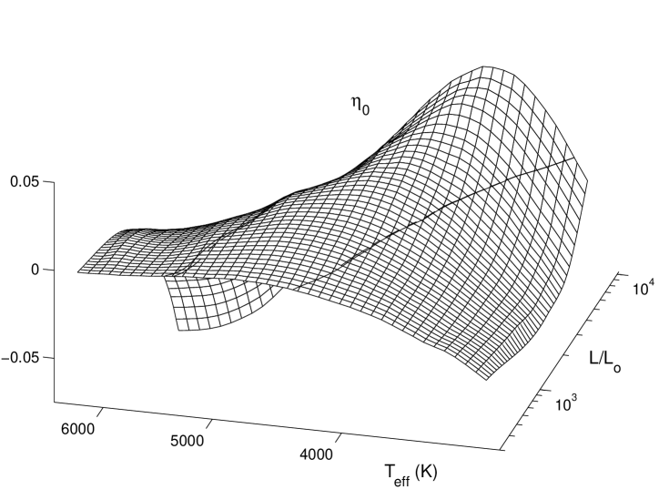
The shape and location of the IS depends on the $\alpha$ parameters that ultimately we want to determine from the observational constraints. To this effect we now calculate Cepheid model sequences with masses in the range $M$=3 – 7$M_{\odot}$. The composition is taken to be $X=0.70$, $Z=0.02$, and $L$ is determined from an assumed mass-luminosity relation $\log L=0.83187+3.56\log M$. At each $M$ (and $L$) a sequence is calculated with $T_{ef\!f}$ ranging from $4000$ to $7000$ K in steps of $100$–$200$ K. At all $M$ and $L(M)$ the $T_{ef\!f}$ dependent growth-rates functionally resemble those of Fig. 8.

The global picture can be visualized in Fig. 12, which shows a typical surface $\eta_{0}=\eta_{0}(L,$$T_{ef\!f}$$)$ (obtained from a cubic spline interpolation of all the computed data). The blue and red edges are shown as contour lines.

We turn now to the morphology of the IS in theoretical HR diagrams as a function of some of the $\alpha$ parameters.

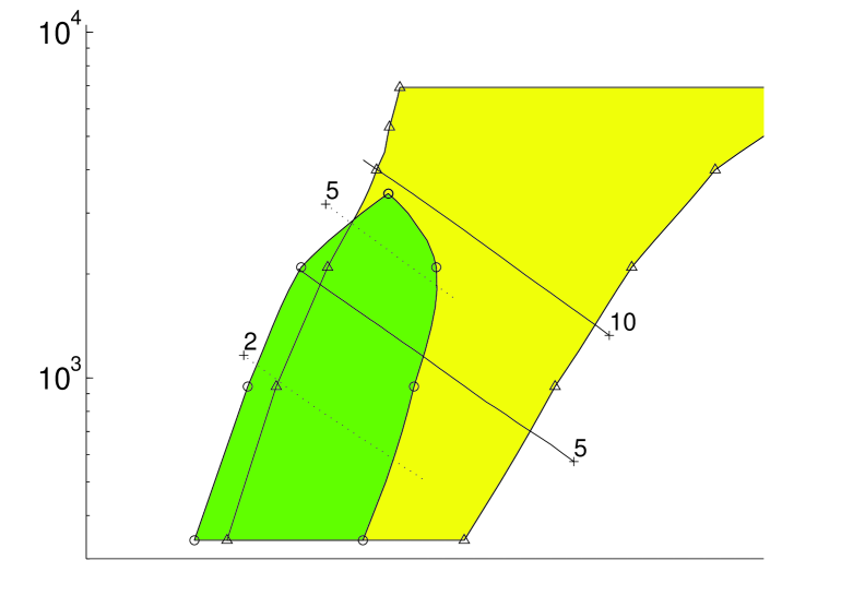
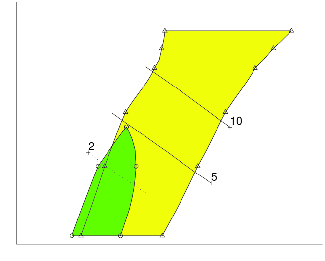
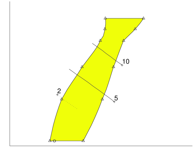
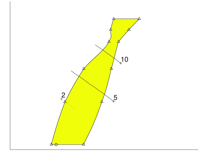
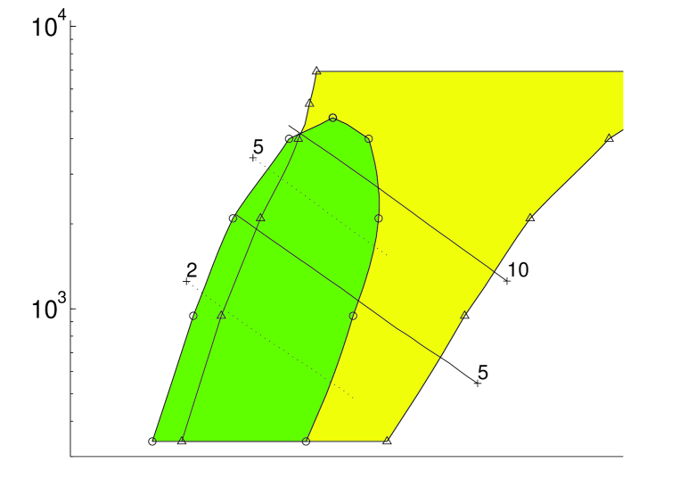
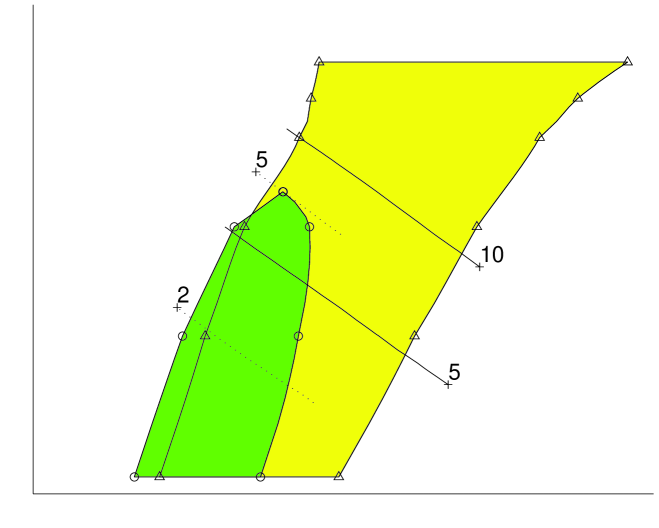
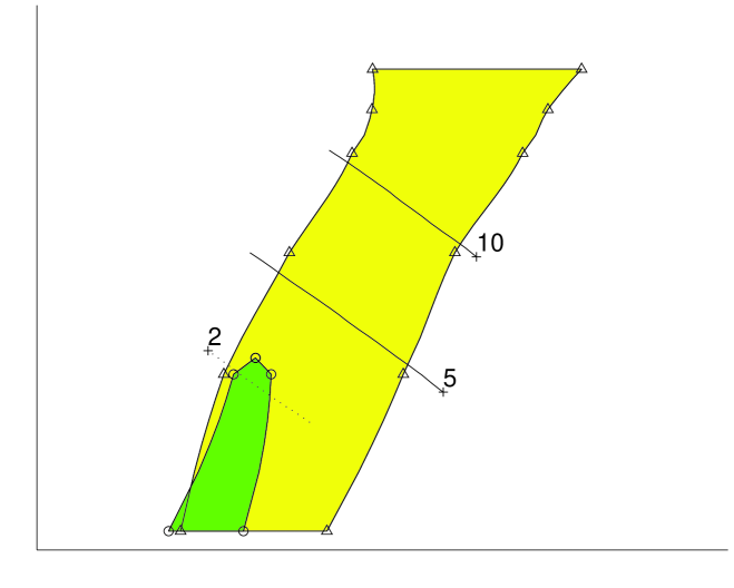
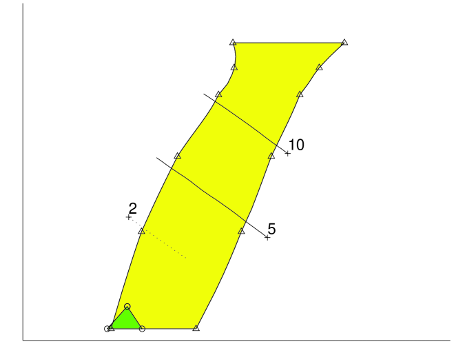
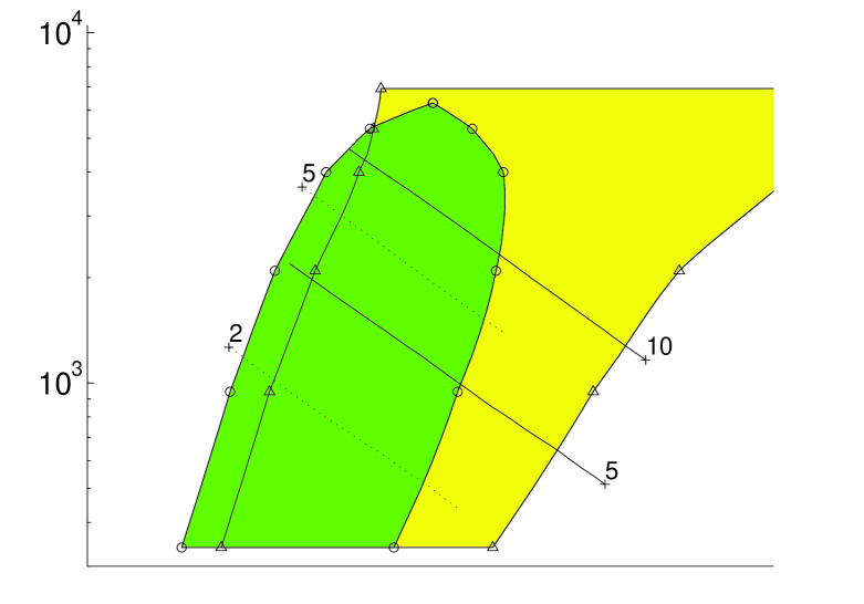
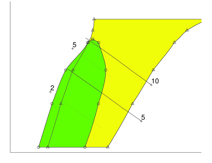
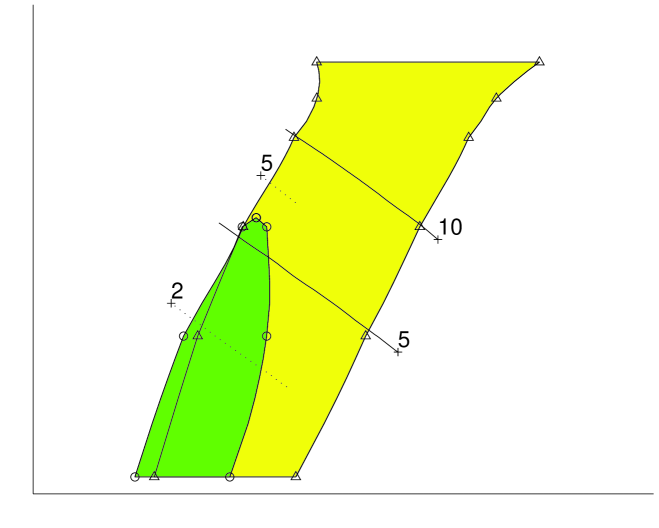
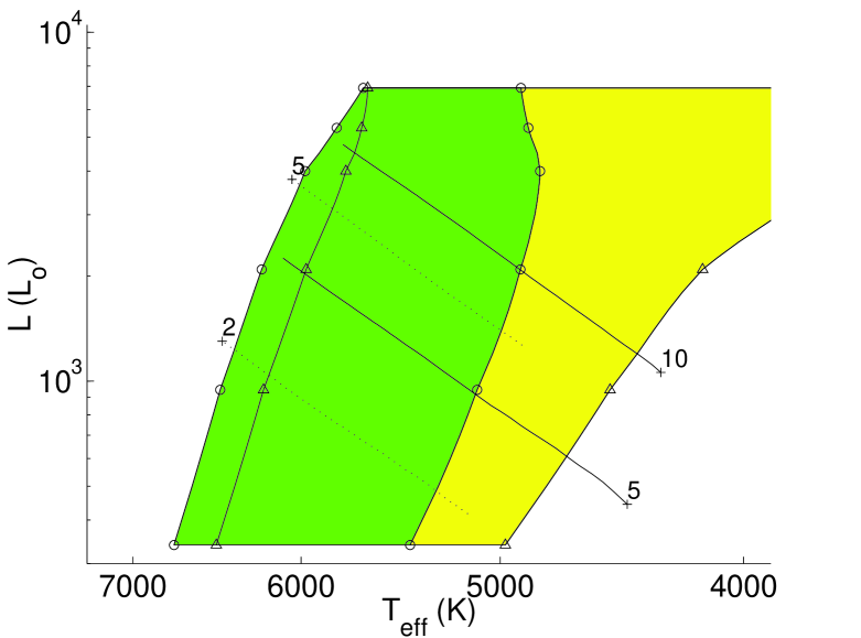
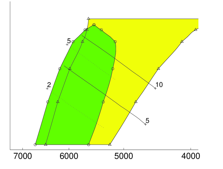
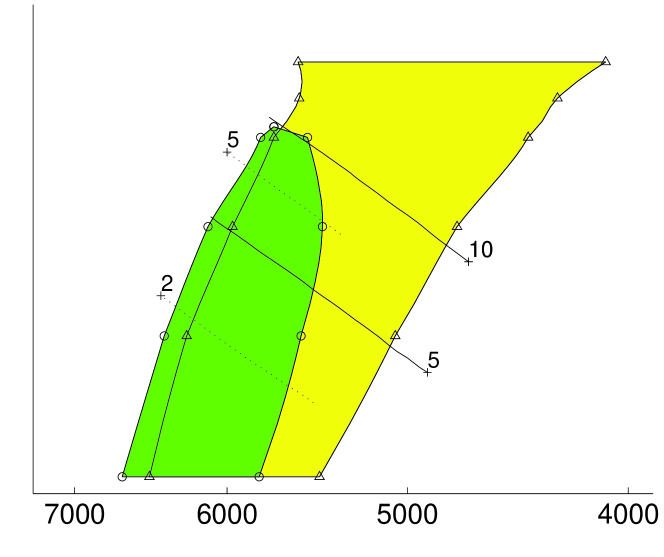
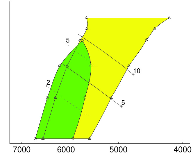
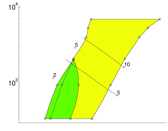
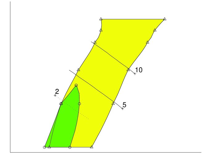
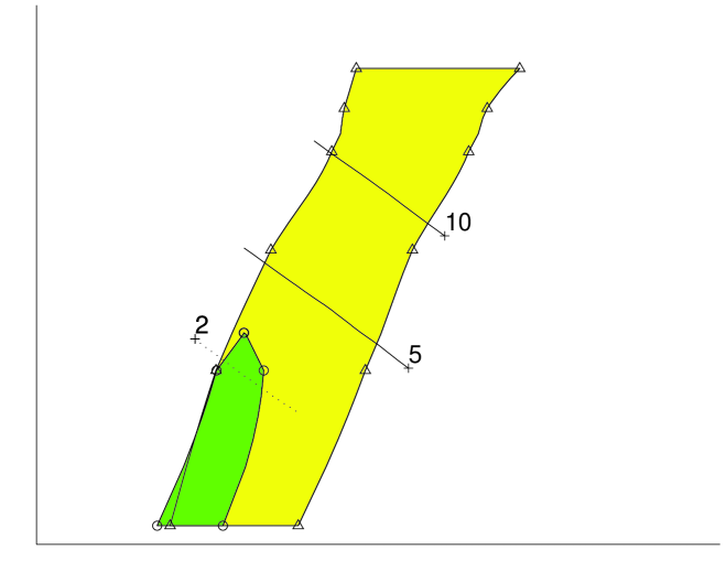
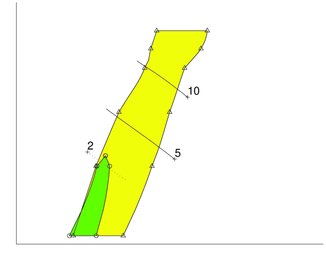
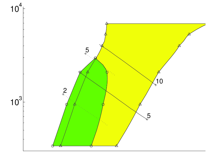
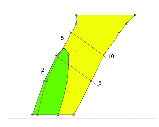
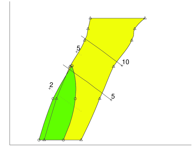
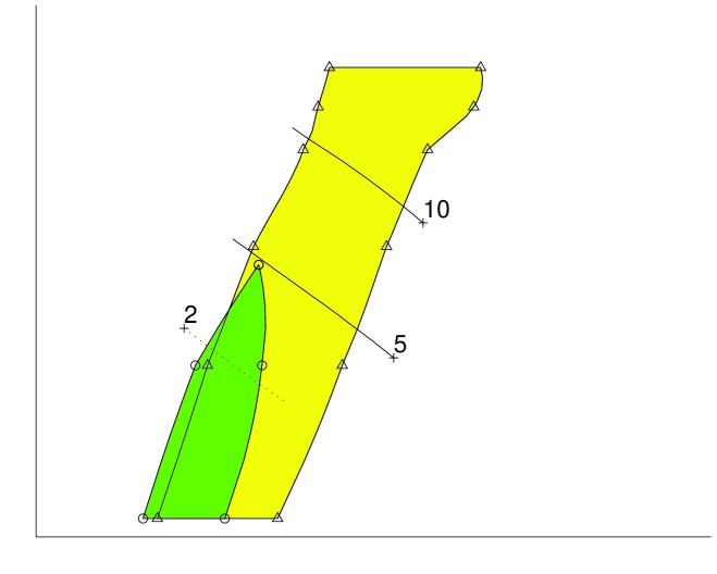
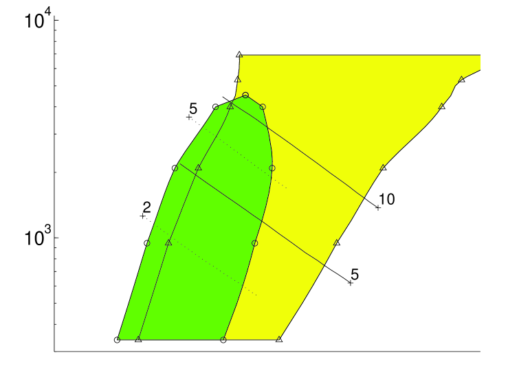
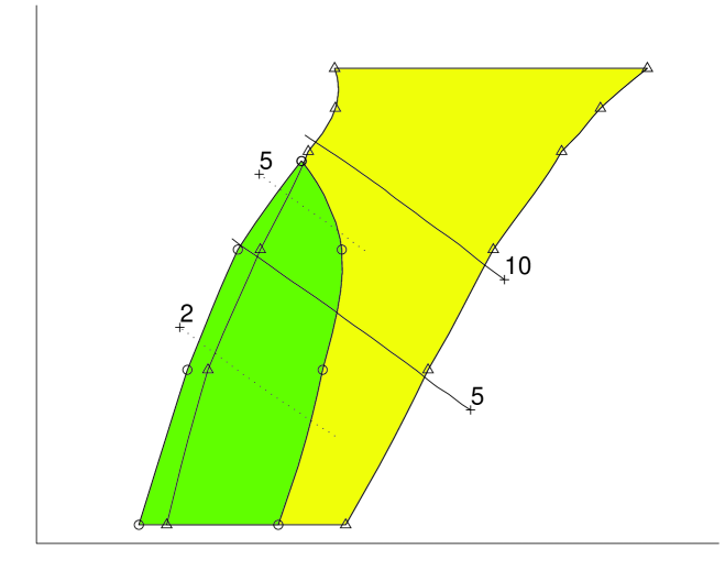
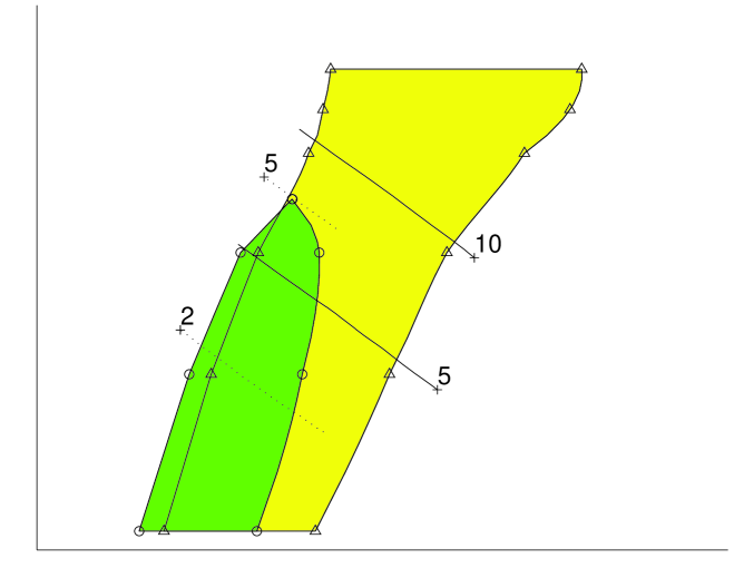
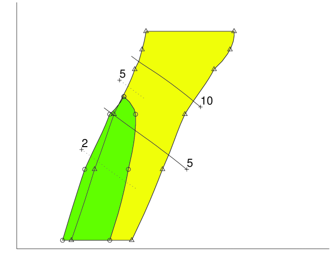
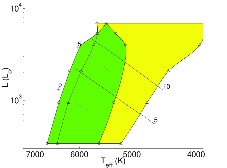
Fig. 13 shows the results for the mixing length parameter $\alpha_{\Lambda}$ (increasing rightward with values 0.288, 0.328, 0.375, 0.390) and $\alpha_{\nu}$ (increasing vertically with values 1.5, 2.0, 2.5, 3.0), and with $\alpha_{c}$=3. (the $\alpha_{p},\alpha_{t},\alpha_{s},\alpha_{d}$ are kept at their standard values). The light-shaded regions form the fundamental IS  ($\eta_{0}>0$) and the dark-shaded ones the first overtone IS  ($\eta_{1}>0$). (The dots represent calculated models, but some of the sharp features are a result of the interpolation and of the relatively crude numerical mesh). One notes that the sensitivity to $\alpha_{\Lambda}$ is very large.

Too weak a convective flux parameter (small $\alpha_{c}$) gives too broad an IS, both for the fundamental (F) and for the first overtone (O1). However, a small mixing length has a similar effect. On the other hand, too large a convective parameter kills off O1. The figure shows that various combinations of parameter values provide approximatively equivalent IS’s, e.g. running approximately from the top middle toward the bottom right.

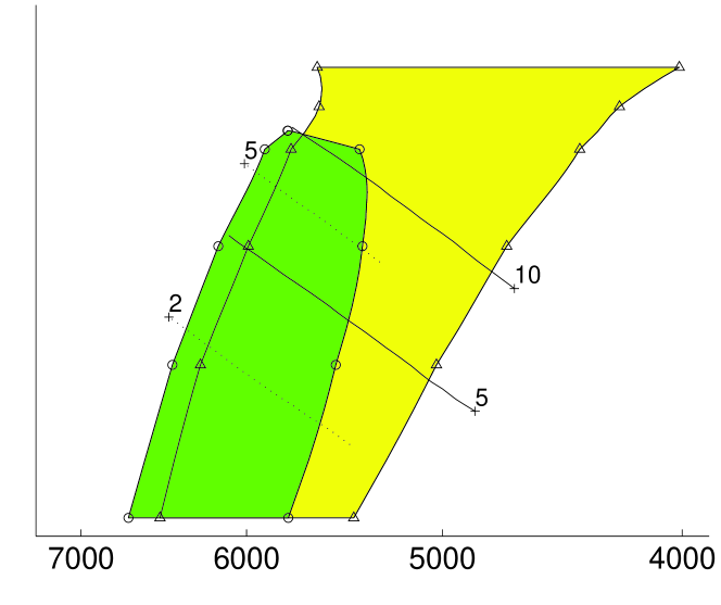
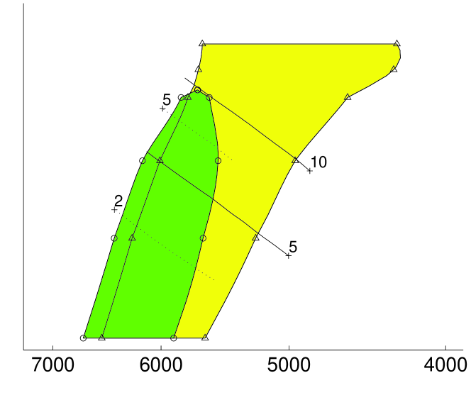
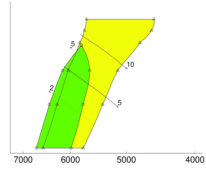
Fig. 14 shows the morphology of the IS in theoretical HR diagrams as a function of the convective flux parameter $\alpha_{c}$ (increasing from left to right with values 2, 3, 4, 5) and $\alpha_{\nu}$ (increasing from the bottom to the top with values 1.0, 1.5, 2.0, 2.5), and with $\alpha_{\Lambda}$ = 0.375 (the $\alpha_{p},\alpha_{s},\alpha_{t},\alpha_{d}$ again are kept at their standard values). This figure again shows that various combinations of parameter values provide approximatively equivalent IS’s, e.g. running approximately from the left top toward the bottom right.

The first overtone IS closes off at large $L$ for some range of $\alpha$ values, which is in agreement with observation. Thus the overtone Cepheids with the longest observed periods ($P_{1}$) give a strong constraint on the value of the $\alpha$’s (and on the $M$ – $L$ relation). For reference we have drawn iso-period lines $P_{0}$ = 5 and 10 d (solid lines) and $P_{1}$ = 2 and 5 d (dotted) in Figs. 13 and 14. Overall, changes in the values of the $\alpha_{c}$ and $\alpha_{\Lambda}$ cause small shifts of the isoperiod lines. As already mentioned most of these shifts are due to the structural rearrangement caused by convection. That is why $\alpha_{\nu}$, which does not appear in the static equilibrium equations, has almost no effect. The periods are only slightly affected by convection near the blue edge, but the pulsation–convection coupling can cause more appreciable changes near the red edge for the more turbulent models.

We conclude that, just from a visual inspection of these IS diagrams, it is possible to delineate the acceptable ranges of the parameters $\alpha_{\Lambda}$, $\alpha_{\nu}$ and $\alpha_{c}$. Roughly speaking the parameters with reasonable looking IS’s lie on a 2D surface in the ($\alpha_{c}$, $\alpha_{\nu}$, $\alpha_{\Lambda}$) parameter space. Table I quantifies this visual result over a more extensive range of the $\alpha$ parameters.

Table 1: Examples of three parameter combinations which give nearly equivalent results for the F and first overtone instability strips.

$\alpha_{c}$		$\alpha_{\Lambda}$		$\alpha_{\nu}$
0.5		0.375		1.50
0.5		0.500		1.00
3.0		0.150		9.00
3.0		0.328		3.00
3.0		0.420		1.00
10.0		0.100		25.00
10.0		0.200		6.00

This flexibility in the $\alpha$ values appears fortunate because ultimately we want not just to fit observed fundamental and first overtone IS’s for the Galaxy, but also for the Magellanic Clouds which have lower $Z$ values. In addition, the wealth of observational Cepheid Fourier decomposition parameters of the (nonlinear) light and radial velocity curves in these galaxies will need to be fitted.

We have thus narrowed down the parameter space on which more detailed calibrations will be made that take into account the wealth of observations. However, we have not made any IS diagrams showing the effects of the other four $\alpha$’s because they seem to play a lesser role, at least at the level of accuracy considered in this parameter survey.

6 Conclusions

Purely radiative Cepheid models cannot satisfactorily account for all observational data, and this has forced us to include turbulence and convection in our Cepheid models. We have adopted a simple 1D model diffusion equation for turbulent convection (TC) that can easily be incorporated into a radial stellar pulsation code. Although there is no guarantee that such a single 1D equation can satisfactorily approximate the effects of turbulence and convection it is worth exploring to what extent we can obtain agreement with observation. The model TC equations contain several dimensionless, order unity parameters that are directly related to the physical quantities of the model that need to be calibrated with the help of observational astronomical constraints.

Instead of performing time-consuming fully nonlinear hydrodynamic computations of the pulsations, we have developed a code to perform an efficient linear nonadiabatic stability analysis of the models. This has allowed us to make an exploration of the sensitivity to the free parameters of the TC equation, both of the structure of the equilibrium Cepheid models and of their linear properties.

In agreement with other studies we find that the static Cepheid models exhibit convection primarily in their H and He partial ionization regions (PIRs), although in some parameter range a convective zone also appears in the Fe PIR. For strongly convective models the separate convective zones merge into a large one that penetrates up to 320,000 K.

The coupling of pulsation and convection also modifies the linear properties of the pulsational modes, as expected. It also creates a new branch of turbulent diffusion modes linear that our stability analysis establishes to be extremely damped, fortunately for our 1D TC recipe. These additional modes thus cannot create havoc numerically or physically. This large damping is consistent with the convective timescales being very short compared to the periods of the vibrational of the excited modes which themselves are short compared to the growth-times.

Our survey shows that the stability of the fundamental and first overtone modes depends on all the TC parameters, but that it is dominated by (1) the convective flux, (2) the eddy viscosity, and (3) the mixing length. Generally, the effects of eddy viscosity and mixing length are greater in the higher overtones.

In agreement with other much less detailed TC studies we find that reasonable $\alpha$ parameter values exist for which IS’s of the galactic Cepheid F and O1 have an acceptable range of temperatures. In this paper we have made no effort to narrow down the acceptable range of TC parameters by using the large amount of observational information. An application of the TC code to a broader sample of Cepheid models and its comparison to the large data base of Galactic, and Magellanic Cloud Cepheids is in progress, as is an extension to RR Lyrae stars.

7 Acknowledgements

This work has been supported by NSF (grants AST95–28338 and INT94–15868). P.Y. gratefully acknowledges helpful conversations with Neil Balmforth and Ed Spiegel.

References

- (1) Balmforth, N.J. 1992, MNRAS 255, 603
- (2) Baker, N.H. 1987, in Physical Processes in Comets, Stars and Active Galaxies, Eds. W. Hillebrandt, E. Meyer-Hofmeister & H.-C. Thomas, p. 105 (Berlin: Springer-Verlag).
- (3) Böhm-Vitense, E. 1958, Zs. f. Ap. 46, 108
- (4) Bono, G. & Stellingwerf, R.F. 1994, ApJ Suppl 93, 233–269
- (5) Bono, G. & Marconi, M. 1997, MNRAS 290, 353
- (6) Buchler, J. R. 1997, in Fifty Years of Stellar Pulsations – A Tribute to Art Cox, Eds. J. Guzik & P. Bradley, ASP (in press)
- (7) Buchler, J.R., Kolláth, Z., Beaulieu, J.P. & Goupil. M.J. 1996, ApJ Letters, 462, L83
- (8) Buchler, J.R., Kolláth, Z. & Marom, A. 1998, ApSpSci, 253, 139
- (9) Canuto, V.M. 1991, ApJ 370, 295
- (10) Castor, J.I. 1968, unpublished preprint
- (11) Castor, J. I. 1971, ApJ, 166, 109
- (12) Gehmeyr, M. 1992, ApJ 399, 265
- (13) Gehmeyr, M. & Winkler, K.-H. A. 1992, AA 253, 92–100; ibid 253, 101–112 [GW]
- (14) Glasner A. & Buchler, J. R. 1993, ApJ 277, 69
- (15) Gonczi, G. & Osaki, Y. 1980, AA 84, 304
- (16) Gough, D.O. 1977, ApJ 214, 196
- (17) Kovács, G. 1990, in The Numerical Modelling of Nonlinear Stellar Pulsations; Problems and Prospects, Ed. J.R. Buchler, NATO ASI Ser. C302, p. 73 (Dordrecht: Kluwer)
- (18) Krishnamurti, R. & Howard, L.N. 1983, Paper in Meteorological Research 6, 143
- (19) Kuhfuss, R. 1986, AA 160, 116
- (20) Rieutord, M. & Zahn, J.-P. 1995, AA 296, 127
- (21) Spiegel, E.A. 1963, ApJ 138, 216
- (22) Spiegel, E.A. 1971, Comments on Astrophysics, 53
- (23) Stellingwerf, R.F. 1974, ApJ, 192, 139
- (24) Stellingwerf, R.F. 1982, ApJ 262, 330
- (25) Unno, W. 1967, Publ Astr Soc Japan 19, 140