Spectral distributions in compact radio sources I. Imaging with VLBI data

Abstract

We discuss a technique for mapping the synchrotron turnover frequency distribution using nearly simultaneous, multi–frequency VLBI observations. The limitations of the technique arising from limited spatial sampling and frequency coverage are investigated. The errors caused by uneven spatial sampling of typical multi–frequency VLBA datasets are estimated through numerical simulations, and are shown to be of the order of 10%, for pixels with the deconvolution ${\rm SNR}\sim 7$. The fitted spectral parameters are corrected for the errors due to limited frequency coverage of VLBI data. First results from mapping the turnover frequency distribution in 3C 345 are presented.

1 Introduction

Information obtained with Very Long Baseline Interferometry (VLBI) about radio spectra of parsec–scale jets and their evolution can be crucial for distinguishing between various jet models. However, there are several aspects of VLBI which impede spectral studies of parsec–scale regions. The reliability of spectral information extracted from VLBI data depends on many factors including sampling functions at different frequencies, alignment of the images, calibration and self–calibration errors, a narrow range of observing frequencies, and source variability. The influences of all these factors must be understood and, if possible, corrected for, in order to reconstruct the spectral properties of parsec–scale jets consistently.

Radio emission from the parsec–scale jets is commonly described by the synchrotron radiation from a relativistic plasma (e.g. Pacholczyk 1970). The corresponding spectral shape, $S(\nu)\propto\nu^{\alpha}$, is characterized by the location of spectral maximum ($S_{\rm m}$, $\nu_{\rm m}$) also called the turnover point, and by the two spectral indices, $\alpha_{\rm thick}$ (for frequencies $\nu\ll\nu_{\rm m}$) and $\alpha_{\rm thin}$ (for $\nu\gg\nu_{\rm m}$).

In many kiloparsec–scale objects, spectral index distributions have been mapped, using observations made with scaled arrays. In such observations, the antenna configurations are selected at each frequency in a specific way such that the spatial samplings of the resulting interferometric measurements are identical at all frequencies used for the observations. It is virtually impossible to use the scaled array technique for VLBI observations of parsec–scale jets made at different frequencies. The uneven spatial samplings of VLBI data at different frequencies result in differences of the corresponding synthesized beams, and can ultimately lead to confusion and spurious features appearing in spectral index maps.

In spectral index maps, the only available kind of information is the spectral slope between the two frequencies. While sufficient for many purposes, this information can be misleading in the situation when the frequency of thespectral maximum lies between the frequencies used for spectral index mapping. In the ranges of frequencies between 1.4 and 43 GHz, frequently used for VLBI observations, such a situation can be quite common. Using observations at three or more frequencies, it is possible to estimate the shape of the synchrotron spectrum, and derive the turnover frequency (frequency of spectral maximum). Information about the turnover frequency can help to avoid the confusion which is likely to occur in spectral index maps. The turnover frequency is sensitive to changes of physical conditions in the jet such as velocity, particle density, and magnetic field strength. This makes it an excellent tool for probing the physics of the jet in more detail than is allowed by analysis of the flux and spectral index properties of the jet.

In this paper, we present a technique suitable for determining the turnover frequency distribution from multi–frequency VLBI data, and investigate its limitations and ranges of applicability. We discuss the advantages of using the Very Long Baseline Array (VLBA) for spectral imaging. A general approach to imaging of VLBA data from nearly simultaneous, snapshot–type observations at different frequencies is outlined in section 2. The effects of limited sampling and uneven uv–coverages are discussed in section 3. We provide analytical estimates of the sensitivity decrease, and use numerical simulations to evaluate the effect the uneven spatial samplings have on the outcome of a comparison of VLBI images at different frequencies. Alignment of VLBI images is reviewed in section 4. A method used for spectral fitting and determining the turnover frequency is described in section 5. Spectral fitting in the case of limited frequency coverage is discussed in section 5.5. The first results from the turnover frequency mapping are presented in section 6.

2 Spectral imaging using VLBA data

Many of the usual technical problems in making spectral index maps from VLBI data can be avoided by using the VLBA (see Zensus, Diamond, & Napier 1995). With the VLBA, it is possible to achieve array homogeneity, have an improved flux calibration, and make the time separation between observations at different frequencies negligible. The major remaining problems are image alignment and uneven spatial samplings of VLBI data taken at different frequencies. At an observing frequency $\nu_{\rm obs}$, the spatial sampling of a baseline $B=\sqrt{B_{X}^{2}+B_{Y}^{2}+B_{Z}^{2}}$ formed by two antennas whose positions differ by $B_{X}$, $B_{Y}$, $B_{Z}$ is characterised by the spatial frequency (e.g. Thompson, Moran & Swenson 1986)

$$\zeta=(\nu_{\rm obs}B/c)\sin\theta_{\rm o}\,,$$ (1)

where $\theta_{\rm o}$ is the angle between the baseline vector and the direction to the observed object. The quantity $\zeta$ is often represented by its coordinate components $u$ and $v$ measured in the spatial frequency plane (uv–plane). The spatial sampling of a VLB array is described by the distribution of spatial frequencies accumulated during the observation at all available baselines (uv–coverage). In VLBI data at different frequencies, these distributions can differ significantly.

To overcome, or at least reduce, the negative effect of uneven uv–coverages, the following scheme of observation and data reduction can be used:

1) Quasi–simultaneous multi–frequency observations. The reliability of interleaved frequency observations can be demonstrated by Figure 1 which compares a VLBI image of 3C345 obtained from a full–track observation and an image made from simulated data that were sampled so that they represent the uv–coverage achieved in a 5/15 duty cycle observation (corresponding to an observation at three frequencies, with 5 minute–long scans at each frequency). Despite some loss of dynamic range and sensitivity, the extended structure is still well detected in the simulated image. The jet appearance in the simulated image is consistent with the jet structures seen in the actual map.

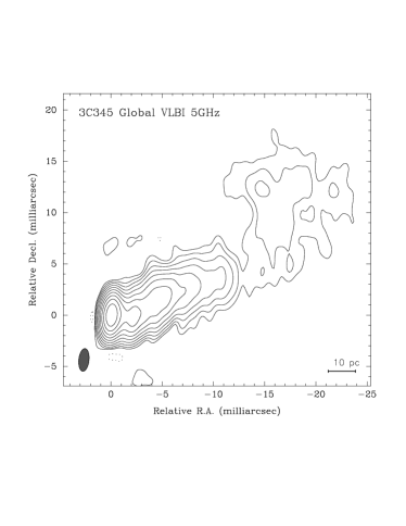
Figure 1: Maps of 3C 345 at 5 GHz (Zensus et al., in prep.) obtained from a real full–track global VLBI observation (top) and from a simulated interleaved–frequency VLBA+VLA observation (bottom). The contour levels are the same in both images: $(-1,1,2,4,8,16,32,64,128,256,512)\times 3.2$ mJy.

2) Careful choice of wavelengths. The choice of wavelengths must be a compromise between the possibility of detecting the source structure and the VLBA sensitivity. Typically, at frequencies higher than 22 GHz, the requirements on brightness temperature limit the sensitivity. Also, there is a stronger dependence of the high frequency data on atmospheric instabilities. At frequencies lower than 2.3 GHz, many sources will become too complicated to warrant a successful structure detection without a full–track observation (see Table 1).

3) Applying the phase–cal information for aligning the relative phases in separate frequency bands (Cotton 1995).

4) Improved amplitude calibration, due to frequent system temperature measurements and a relatively weak elevation dependence of the power gains of the VLBA antennas (Moran & Dhawan 1995).

Table 1: Maximum sampling intervals [min] and maximum detectable structure sizes [mas] for a 8600 km–long baseline.

8600-km baseline
$\nu$	structure size (mas)								sampling interval (min.)
${\rm[GHz]}$	1	3	5	10	20	30	50	100	10	15	20	25	30	35	40	50
43.2	19	6.5	4.0	2.0	1.0	0.5	0.3	0.2	1.9	1.3	1.0	0.8	0.7	0.6	0.5	0.4
22.2	36	12	7.0	3.5	1.8	1.2	0.7	0.4	3.5	2.4	1.8	1.4	1.2	1.0	0.9	0.7
15.1	55	18	11	5.5	2.7	1.8	1.1	0.6	5.5	3.8	2.7	2.2	1.8	1.6	1.4	1.1
8.4	110	38	22	11	5.5	4.0	2.5	1.0	11	7.0	5.5	4.4	3.8	3.2	2.7	2.2
5.0	160	55	32	16	8.0	5.5	3.0	1.5	17	11	8.0	6.5	5.5	4.6	4.0	3.2
2.3	360	120	70	35	18	12	7.0	3.5	35	24	18	14	12	10	9.0	7.0
1.6	…	180	110	55	27	18	11	5.5	55	38	27	22	18	16	14	11
0.6	…	…	280	140	70	46	28	14	140	95	70	55	47	40	35	28
0.3	…	…	…	240	120	80	50	25	240	160	120	100	80	70	60	50
	maximum sampling interval (min.)								largest detectable structure (mas)

5) Applying appropriate uv–tapering, in order to provide matching uv-ranges for data taken at different frequencies.

6) Convolving data at different frequencies with the same, artificially circular beam.

7) Using SNR and flux threshold cutoffs, in order to leave out the remaining sidelobe–induced artifacts.

8) If strong sidelobe effects remain present, matching the uv–coverages within certain uv–ranges or over the whole uv–plane.

3 Spatial sampling

Two effects are specific to the observing scheme described above: the decrease in sensitivity due to reduced uv–sampling at each observing frequency, and uneven spatial samplings at different observing frequencies. In this section, we investigate the effect of these factors on VLBI data at different frequencies.

With a larger number of antennas, the overlapping parts of the uv–coverages at different observing frequencies constitute an increasingly larger fraction of the joint uv–population. This results in decreasing the flux density level at which the confusion effects dominate the results of spectral index calculations. The confusion level can be lowered further by applying specific weighting schemes to the data (uv–weighting), and by matching the ranges of the uv–coverages at both frequencies. In the spectral index maps produced using the above procedures, confusion occurs at the flux level of about 0.3–0.5% of the mean peak flux density in the corresponding total intensity maps (Lobanov 1996).

3.1 Longest sampling intervals and largest detectable structures

For a given time sampling interval $\Delta t$, an estimate of the largest angular size, $\Omega_{\rm max}$, of structures that can be detected on a baseline $B$ can be calculated from the time–average smearing (Bridle & Schwab 1989). The sensitivity reduction is greatest when the apparent motion of the source is perpendicular to the fringes associated with the selected baseline, and so we can assume a polar source and an East–West oriented baseline, in order to provide the most conservative estimates of $\Omega_{\rm max}$. This gives

$$\Omega_{\rm max}=\frac{\nu_{\rm obs}}{\omega_{e}c\Delta t(B_{X}^{2}+B_{Y}^{2})^{1/2}}\,,$$ (2)

with $\omega_{e}$ denoting the Earth angular rotation speed. For a feature located at the sky coordinates $l$, $m$ with respect to the phase–tracking center (Thompson, Moran & Swenson 1986), the corresponding average reduction in amplitude over a 12–hour period is

$$<R_{\Delta t}>=<I/I_{0}>\approx 1-\frac{\pi^{2}}{12\Omega_{\rm max}^{2}}(l^{2}+m^{2}\sin^{2}\delta)\,,$$ (3)

where $\delta$ is the source declination.

Table 2: Parameters of a typical VLBA and VLA antennas

Freq.	$T_{\rm sys}$	K	SEFD	$\eta$	$\sigma_{\rm therm}$	Freq.	$T_{\rm sys}$	K	SEFD	$\eta$	$\sigma_{\rm therm}$
$[$GHz$]$	[K]	[K Jy-1]	[Jy]		[Jy]	$[$GHz$]$	[K]	[K Jy-1]	[Jy]		[Jy]
VLBA 0.3	213	0.100	2162	0.45	0.086	VLA 0.3	150	0.071	2113	0.40	0.068
0.6	192	0.086	2207	0.40	0.087	0.6	…	…	…	…	…
1.6	29	0.095	303	0.57	0.009	1.6	37	0.091	406	0.51	0.013
2.3	29	0.091	315	0.50	0.010	2.3	…	…	…	…	…
5.0	38	0.130	291	0.72	0.010	5.0	44	0.116	379	0.65	0.012
8.4	35	0.117	304	0.70	0.009	8.4	34	0.110	309	0.63	0.010
15.1	57	0.111	514	0.50	0.021	15.1	110	0.093	1183	0.52	0.039
22.2	93	0.102	945	0.60	0.028	22.2	140	0.082	1707	0.45	0.057
43.2	107	0.084	1348	0.52	0.038	43.2	90	0.030	3000	0.37	0.044

For every combination of wavelength and structure size, the left panel of Table 1 gives the corresponding maximum allowed sampling interval [in minutes] between individual scans. Dots indicate that a structure remains unresolved. Italics highlight the 50% decrease of sensitivity. The right panel of Table 1 gives the expected maximum size of detectable structure [in mas], for all combinations of wavelengths and sampling intervals. The calculations have been done for the longest available VLBA baseline ($B_{\rm L}=8600$ km). Here we postulated $B_{Z}=0$ and $B_{\rm L}^{2}=B_{X}^{2}+B_{Y}^{2}$, to provide more restrictive estimates.

It follows from Table 1 that multi–frequency observations can provide satisfactory structure and flux sensitivities for bright sources with intermediate ($\approx 10$ mas) extension. For such sources, full–scale spectral index mapping with 5 minute–long scans can be done at frequencies lower than 43 GHz (0.7 cm).

3.2 Simulations of multi–frequency VLBA data

To study the effect of uneven uv–coverages on spectral imaging, we simulate visibility data at all frequencies available at the VLBA, using the routine “FAKE” from CIT VLBI package (Pearson 1991). At all frequencies, the simulated data are produced from the same “CLEAN” (Cornwell & Braun 1989) $\delta$–component model of the structure in the top panel of Figure 1. To improve short–spacing coverage, we include one VLA antenna in the simulations. The simulated bandwidth, $W=64$ MHz, corresponds to one of the standard VLBA observing modes (128 Mb s^-1 data rate with 1 bit sampling; Romney 1992). We model the antenna efficiencies, $\eta_{i}$ (Crane & Napier 1989), using the antenna sensitivities, $K_{i}$ (Crane & Napier 1989), and the mean VLBA values, $\eta_{\rm VLBA}$ and $K_{\rm VLBA}$, given in Napier (1995). Then, for each VLBA antenna, the resulting efficiency is:

$$\eta_{i}=\eta_{\rm VLBA}(K_{i}/K_{\rm VLBA})\,.$$ (4)

The system equivalent flux densities, $SEFD$, are calculated from the antenna sensitivities and system temperatures, $T_{\rm sys}$: $SEFD_{i}=T_{\rm sys,i}/K_{i}$ (Walker 1995; Crane & Napier 1989).

To make the simulated data as realistic as possible, we introduce four types of errors: the Gaussian additive noise, $\sigma_{\rm therm}$, Gaussian multiplicative noise $\sigma_{\rm m}$, gain scaling errors $\sigma_{\rm gain}$, and random station–dependent phase errors. Both $\sigma_{\rm m}$ and $\sigma_{\rm gain}$ are chosen to be at a 2% level, which is a good approximation of typical VLBA gain calibration errors.

For a bandwidth of $W$[MHz] and integration time of $\tau_{\rm int}$[s], the additive Gaussian noise can be calculated for each antenna, using the antenna zenith system temperatures, $T_{\rm sys}$, and antenna efficiencies $\eta$. We have

$$\sigma_{\rm therm}=5T_{\rm sys}/(\eta\epsilon_{\rm pt}D_{\rm ant}^{2}\sqrt{\tau_{\rm int}W})\,,$$ (5)

where $D_{\rm ant}=25$ m is the antenna diameter, and $\epsilon_{\rm pt}$ is the pointing efficiency. The pointing efficiency can be estimated from the ratio of pointing errors, $\sigma_{\rm pt}$, to the half–power beamwidth of an antenna at a given frequency. The typical non–systematic pointing errors of VLBA antennas are within $8$–$14\arcsec$ (Romney 1992), which results in $\epsilon_{\rm pt}\sim 85$–$99\%$ at most of the VLBA observing frequencies. The overall parameters used in the data simulations are summarized in Table 2 for a typical VLBA (Wrobel 1997) and VLA antennas.

Figure 2: Baseline visibility amplitudes on the baseline between VLBA antennas at Los Alamos and North Liberty. Top panel shows data from a real observation; simulated data are shown in the bottom panel.

Using the parameters from Table 2, and adding the errors described above, we simulate VLBA visibility datasets that would be obtained in an observation with a 5/15 duty cycle corresponding to observing at 3 frequencies, with 5 minute long scans at each frequency. We simulate a 17 hour–long observation of 3C 345, with 30 second averaging time for individual data points—similar to the typical duration and averaging time of real VLBI observations. The simulated data at 5 GHz are compared in Figure 2 with the data from a real VLBI observation, for a VLBA baseline Los Alamos – North Liberty. One can see that the noise levels are comparable in the real and simulated data.

3.3 Spatial sampling at different frequencies

To study the effects of uneven uv–coverages in VLBI data, we image the simulated datasets, following the procedure described in section 2. An image obtained from the simulated data at 5 GHz is shown in the lower panel of Figure 1. Flux density and spectral index errors due to differences in spatial samplings can be estimated from comparison of the images made from the simulated data at different frequencies. In the ideal case, the flux ratio measured between any two images should remain unity in every pixel, and the corresponding spectral index should be zero across the entire image. Since all images are produced from the same source model, we ascribe all deviations from zero spectral index to the errors due to different spatial samplings and random errors, and choose to present these errors as a function of pixel SNR measured with respect to the self–calibration noise. The latter is taken to be equal to the largest negative pixel in the map, and is approximately 5–10 times bigger than the formal RMS noise of the image. In the simulated data, the average self–calibration noise is $\approx 5$ mJy.

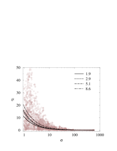
Figure 3: Fractional errors due to different uv–coverages. The errors are plotted against the pixel flux scaled to the average self–calibration noise, $\sigma=5$ mJy.

Figure 3 shows the fractional errors as a function of pixel SNR. We plot the results from all image pairs together (5, 8, 15, 22, and 43 GHz data are used). The curved lines represent power law fits to the individual image pairs; the frequency ratio of each pair is given in the legend. The errors increase significantly at SNR$\leq 7$. We find that pixel SNR is the main factor determining the derived errors, although the errors in pixels with comparable SNR tend to increase slightly at larger distances from the phase center. This increase however is considerably weaker compared to the increase of errors due to lower pixel SNR.

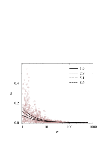
Figure 4: Errors in spectral index due to different uv–coverages. The errors are plotted against the pixel flux scaled to the average self–calibration noise, $\sigma=5$ mJy.

The spectral index errors are shown in Figure 4 for the same image pairs. Similarly to the fractional errors, the magnitude of spectral index errors increases rapidly at low SNR. The main difference is that the errors become progressively smaller at larger frequency separations, which follows obviously from the definition of the spectral index.

From the error distributions shown in Figures 3–4, we conclude that multi–frequency VLBA observations with the time sampling interval of 10 minutes at each frequency can be compared with each other, for pixels which are located at moderate ($\sim 10$–15 mas) distances from the phase–tracking center, and have a sufficiently high SNR ($\mathrel{\raise 1.72218pt\hbox{\hbox to0.0pt{$>$\hss}\lower 5.16663pt\hbox{$\sim$}}}5$). Within these limits (and with the applied observing and data reduction strategy), the fractional errors should not exceed $\sim$10%, a precision that can be sufficient for several purposes including spectral index and turnover frequency mapping in the nuclear regions of parsec–scale jets. Most of the large amplitude errors occur at jet edges where the effects of uneven spatial samplings are most pronounced. This effect is readily confirmed by Figure 5 in which the distribution of fractional errors is plotted for the 5–15 GHz image pair. The contours outline areas in which the errors are larger than 5%. These areas are concentrated at the jet edges, and cover a fairly small fraction of the entire source structure.

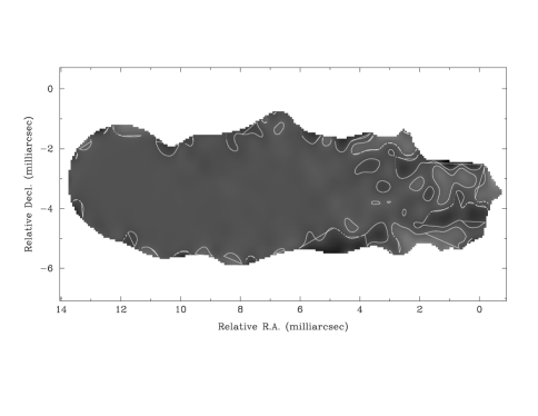
Figure 5: Distribution of fractional errors in a 5–15 GHz image pair. Contours outline the regions with errors larger than 5%.

4 Image alignment

Position measurements with the precision required for the alignment of VLBI images cannot be made without extensive absolute or relative astrometry observations. In quasi–simultaneous multi–frequency VLBI observations, the phase–referencing technique bc95 (Beasley & Conway 1995) can be sufficient for the purpose of image alignment. If neither of the aforementioned techniques is available, VLBI images are usually aligned by means of the position of compact core of the source. The core is likely to be located in an optically thick environment, and its position must depend on the observing frequency, $\nu$. According to Königl (1981), the core is observed at the separation $r_{\rm core}\propto\nu^{-1/k_{r}}$ from the true jet origin. The term $k_{r}$ is close to unity (Marcaide et al. 1985, Lobanov 1997), so that $r_{\rm core}$ depends almost inversely on the frequency. Therefore, if aligned by the position of the core, VLBI images may contain systematic position offsets undermining spectral imaging.

The frequency dependent shift of the core position can be deduced from comparison of observations made at close epochs, assuming that the superluminal features observed in the jet are optically thin and therefore should have their positions unchanged. In this case, the offsets between the component locations measured at different frequencies will reflect the respective shift of the observed position of the optically thick core. This approach has been successfully used in several studies (e.g. Biretta et al. 1986; Zensus et al. 1995; Lobanov 1997), and we deem it to be sufficient for the purpose of aligning VLBI images at different frequencies.

5 Spectral fitting

The frequency range covered by VLBI observations is very narrow (roughly, from 1 to 100 GHz, with most of the observations done between 5 and 22 GHz). The turnover frequency, $\nu_{\rm m}$, of the synchrotron spectrum often lies outside the range of observing frequencies (see the sketch in Figure 6). Because of the limited frequency coverage, a straightforward application of the synchrotron spectral form to fitting may be ill–constrained (such as in the case B in Figure 6). To provide an estimate of $\nu_{\rm m}$ in such cases, we first attempt to achieve the best fit of spectral data by polynomial functions, and then analyse local curvature of the obtained fit. From the measured curvature, an estimate (often only an upper limit) of $\nu_{\rm m}$ can be found. Details of spectral fitting are given in section 5.4; application of the local curvature for determining the turnover frequency is discussed in sections 5.5–5.6.

Figure 6: Sketch illustrating the problems existing in determining the turnover frequency from VLBI data with insufficient frequency coverage. A homogeneous synchrotron source with isotropic pitch angle distribution is assumed. When the true turnover frequency lies outside of the range of observing frequencies, ad hoc information about low and high–frequency spectral shape is required, as well as the second order corrections based on the measured curvature of the observed part of the spectrum (see text for details).

5.1 Basic synchrotron spectrum

For an extensive coverage of synchrotron emission and its properties, we refer to the works by Ginzburg and Syrovatskii (1969), Pacholczyk (1970), and Ternov and Mikhailin (1986). In our calculations, we consider synchrotron emission from a homogeneous plasma with isotropic pitch angle distribution and power law energy distribution $n(\gamma)d\gamma=n_{\gamma_{0}}\gamma^{-s}d\gamma$, for electron Lorentz factors $\gamma_{\rm L}<\gamma<\gamma_{\rm H}$. In this case, it would suffice to describe the emission within the range of frequencies $\nu_{\rm L}\ll\nu\ll\nu_{\rm H}$, where $\nu_{\rm L,H}$ are the low–frequency and high–frequency cutoffs given by:

$$\nu_{\rm L,H}\approx\gamma^{2}_{\rm L,H}\frac{\Omega_{e}}{\pi},$$ (6)

where $\Omega_{e}$ is the electron gyro–frequency. Then, for a plasma with electron self–absorption, the spectral distribution of emission is (Pacholczyk 1970):

$$I_{\nu}\propto\left(\frac{\nu}{\nu_{1}}\right)^{\alpha_{\rm t}}\left\{1-\exp\left[-\left(\frac{\nu_{1}}{\nu}\right)^{\alpha_{\rm t}-\alpha_{\rm o}}\right]\right\},$$ (7)

where $\nu_{1}$ is the frequency at which the optical depth, $\tau_{\rm s}=1$, and $\alpha_{\rm t}$, $\alpha_{\rm o}$ are the spectral indices of the optically thick and optically thin parts of the spectrum (with spectral index defined by $S\propto\nu^{\alpha}$). It is clear from equation 7 that at frequencies $\nu\ll\nu_{1}$: $I_{\nu}\propto(\nu/\nu_{1})^{\alpha_{\rm t}}$; and at frequencies $\nu\gg\nu_{1}$: $I_{\nu}\propto 1-\exp[-(\nu_{1}/\nu)^{\alpha_{\rm t}-\alpha_{\rm o}}]$. For a plasma with a homogeneous synchrotron spectrum $\alpha_{\rm t}=2.5$. We will use the above $\alpha_{\rm t}$ and the description given by (7) in our calculations.

5.2 Fitting algorithm

The main steps of spectral fitting can be summarized as follows:

1) Make an approximate estimate of cutoffs in the spectrum, on the basis of all available spectral information. A fairly good guess can be attained by taking the average measured turnover frequency and optically thin spectral index in the compact source. Based on these values, calculate the high and low frequencies at which the corresponding flux density is at an arbitrarily low level (we use $S_{\rm cutoff}=0.1$ mJy). Add these spectral points to the measured data in each pixel, in order to ensure a negative curvature of the fitted curves, as required by the theoretical spectral form (7).

2) Fit the combined pixel spectra by polynomial functions, allowing for limited variations of the cutoff frequencies, and aiming at achieving the best fit to the measured data points. From the fits, determine the basic spectral parameters: the turnover frequency, turnover flux density, and integrated flux (with integration limited to the range of observing frequencies). Estimate the errors from Monte Carlo simulations, using the distribution of the $\chi^{2}$ parameters of the fits to the simulated datasets.

3. Calculate the local curvature of the fitted spectra within the range of observing frequencies. Compare the derived curvature with the values obtained from analytical or numerical calculations of the synchrotron spectrum. Derive the corrected value of the turnover frequency, by equating the fitted and the theoretical spectral curvatures.

4. Fit the data with the synchrotron spectral form described by (7), and using the corrected value of the turnover frequency.

The above procedure has been applied to spectral data obtained from modelling VLBI images of 3C 345 by elliptical Gaussian components, and combining the models at different frequencies (Lobanov & Zensus 1998).

5.3 Spectral cutoffs

Because the transition between high–frequency ($\nu>\nu_{1}$) and low–frequency ($\nu<\nu_{1}$) spectral regimes determined by equation 7 is very sharp, the spectrum is determined by the synchrotron self–absorption at frequencies $\nu\ll\nu_{1}$, and by the electron energy distribution at $\nu\gg\nu_{1}$. Estimates of the typical turnover frequency and energy spectral index in the jet of 3C345 based on our own calculations and on the results from Rabaça and Zensus (1994) give $\nu_{1}\approx 10$ GHz and $s\approx 2.6$. Using these values, we estimate the low–frequency, $\nu_{\rm L}\sim$ 1 MHz, and high–frequency, $\nu_{\rm H}\sim$ 1000 GHz, cutoffs in the spectrum, and use these values for the spectral fitting. However, the cutoffs cannot be well defined, and may change during the evolution of the jet emission. To account for this effect, we allow 15% variations of the cutoff frequencies so as to achieve the best fit to the data.

5.4 Spectral fits

In order to calculate the spectral parameters of jet emission, we combine the component fluxes measured at frequencies $\nu_{1},...,\nu_{\rm N}$, and add the cutoff information. The resulting spectral dataset ${S_{s},\sigma_{s}^{2}}$ is represented by the flux densities,

$$\{S_{s}\}=\{S(\nu_{\rm L}),S(\nu_{1}),...,S(\nu_{\rm N}),S(\nu_{\rm H})\}\,,$$

and their respective variances,

$$\{\sigma^{2}_{s}\}=\{\sigma^{2}_{S}(\nu_{\rm L}),\sigma^{2}_{S}(\nu_{1}),...,\sigma^{2}_{S}(\nu_{\rm N}),\sigma^{2}_{S}(\nu_{\rm H})\}\,,$$

where $S(\nu_{\rm L})=S(\nu_{\rm H})=0.1$ mJy is the cutoff flux density level.

By varying the spectral dataset, we then produce simulated spectral datasets

$$S_{\rm sym}={\cal V}(S_{s})|_{\{\sigma^{2}_{\rm S}(\nu)\}}$$ (8)

assuming the Gaussian distribution of the errors in flux density measurements

$$\phi(S)=\frac{1}{\sqrt{2\pi}\sigma_{\nu}}e^{-1/2\left(\frac{S-S_{\nu}}{\sigma_{\nu}}\right)^{2}}$$ (9)

where $S_{\nu}$ and $\sigma_{\nu}$ are the measured flux density and its variance.

For each simulated spectral dataset, we apply the $M^{th}$–order ($M\leq N-1$) polynomial fitting by the basis functions $X_{k}(\nu)=\nu^{k}$, and minimize the $\chi^{2}$ parameter of the fit

$$\chi^{2}=\sum^{N}_{i=1}\frac{1}{\sigma^{2}_{i}}\left[(S_{\rm sym})_{i}-\sum^{M}_{k=0}A_{k}X_{k}(\nu_{i})\right]^{2},$$ (10)

to obtain the least squares fit to the data, and derive the polynomial coefficients

$$A_{j}=\sum^{M}_{k=0}[a]^{-1}_{jk}\beta_{k},\quad\sigma^{2}(A_{j})=[a]{-1}_{jj}\,.$$ (11)

Here $a_{j,k}$ and $\beta_{k}$ are given by

$$a_{j,k}=\sum^{N}_{i=1}\frac{X_{j}(\nu_{i})X_{k}(\nu_{i})}{\sigma_{i}^{2}},$$

$$\beta_{k}=\sum^{N}_{i=1}\frac{(S_{\rm sym})_{i}X_{k}(\nu_{i})}{\sigma_{i}^{2}}\,.$$

From the fit to the spectral dataset, we derive the basic parameters of the synchrotron spectrum: the integrated flux,

$$S_{\rm int}=\int_{\nu_{1}}^{\nu_{\rm N}}\sum_{j=0}^{M}A_{j}\nu^{j}d\nu\,,$$ (12)

the turnover frequency, $\nu_{\rm m}$, and the turnover flux density, $S_{\rm m}$:

$$\frac{{\rm d}\sum_{j=0}^{M}A_{j}\nu^{j}}{{\rm d}\nu}=0\;\Rightarrow\;S_{\rm m},\nu_{\rm m}$$ (13)

We then analyse the distribution of the $\chi^{2}$ parameters from the fits to all simulated datasets. From this analysis, standard deviations at the $3\sigma$ confidence level are calculated for $S_{\rm int}$, $S_{\rm m}$, and $\nu_{\rm m}$.

5.5 Curvature of the fits

Figure 7: Theoretical curvature, $\kappa$, of the homogeneous synchrotron spectrum with spectral index $\alpha$. The $\xi$ axis denotes the ratio of the frequency at which the curvature is calculated to the turnover frequency.

Figure 8: Curvature correction coefficients derived from simulating synchrotron spectra and subsequent fitting them by the polynomial functions described in section 5.4.

The local curvature of spectral fits is:

$$\kappa=\frac{{\rm d}^{2}S}{{\rm d}\nu^{2}}\left[1+\left(\frac{{\rm d}S}{{\rm d}\nu}\right)^{2}\right]^{-1/3}\,.$$ (14)

The mathematical details of calculations are summarized in Appendix. If the spectral index, $\alpha_{\rm o}$, and the local curvature, $\kappa_{\rm o}$, of a polynomial fit are determined at a frequency $\nu_{\rm o}$, then the turnover frequency, $\nu_{\rm m}$, can be estimated from the adopted theoretical synchrotron spectrum. Using the derived $\alpha_{\rm o}$ and $\kappa_{\rm o}$, we determine the ratio $\xi(\alpha_{\rm o},\kappa_{\rm o})=\nu_{\rm m}/\nu_{\rm o}$, from the adopted spectral form described by (7). The corresponding turnover frequency is then

$$\nu_{\rm m}=\nu_{\rm o}\xi(\alpha_{\rm o},\kappa_{\rm o})\,.$$ (15)

Figure 7 relates the curvature $\kappa$ of the homogeneous synchrotron spectrum described by (7) to the ratio $\xi(\alpha_{\rm o},\kappa_{\rm o})$. For frequencies increasingly deviating from the turnover frequency (for which $\xi=1$), the curvature, $\kappa$, becomes progressively smaller, thereby limiting the ranges of applicability of the corrections described by (15). For data covering the frequencies from $\nu_{1}$ to $\nu_{\rm N}$, we expect the corrections to give reliable estimates for the turnover frequencies lying within the $0.05\nu_{1}<\nu_{\rm m}<2\nu_{\rm N}$ range.

5.6 Numerical estimates of the curvature corrections

An alternative method to estimate $\xi(\alpha_{\rm o},\kappa_{\rm o})$ is to determine it numerically, by simulating the synchrotron spectrum with given turnover frequency and spectral index, and fitting it by the polynomial functions used in section 5.4. We have performed such calculations, using the spectral form described in section 5.1, and covering a range of turnover frequencies and spectral indices. The results are shown in Figure 8 in which the ratio of fitted values to the theoretical values of the turnover frequency is plotted against the synchrotron spectral index. The contours show different values of $\xi$. One can see that the determined ratios do not depend strongly on the spectral index. Figure 8 can be used for the same purpose of correcting the fitted turnover frequencies obtained through the procedure described in section 5.4.

Figure 9: Maps of 3C 345 from the multi–frequency VLBA observation made on June 24, 1995. The restoring beam is 1.2$\times$1.2 mas. The contours are (1,1.4,2,2.8, 4,…,51.2)$\times$14 mJy.

6 Turnover frequency mapping

On the basis of the method described above, we have developed a code for mapping the turnover frequency distribution from multi–frequency VLBA data. Fitting is performed in every valid pixel of the image; the validation is based on clipping the pixels with low flux density or low SNR. Flux density errors are estimated from the noise level and flux density gradients in the total intensity maps. For each pixel, we average the values of pixels within selected bin, and add, in quadratures, the averaging standard deviations to the estimated noise level. This results in slightly increased errors for pixels in the areas with steep flux density gradients, providing more conservative error estimates. The use of the gradients for error estimation is optional, and can be turned off by setting the bin size to 1.

The output of the mapping procedure can be the turnover frequency distribution, turnover flux density distribution, integrated flux distribution, or total intensity map at a given frequency. The last option allows us to predict, from the fitted spectral shape, the expected source structure at any frequency within the range of observing frequencies of the maps used for the spectral fitting. This can also be used for testing the quality of the spectral fit, by comparing the predicted and observed images at the same frequency (given that the observed image was not used for producing the above spectral fit).

Table 3: Parameters of the VLBA maps

1	2	3	4	5	6	7	8
$\nu_{\rm obs}$	$S_{\rm tot}$	$S_{\rm peak}$	$S_{\rm neg}$	$S_{\rm noise}^{\rm est}$	Beam	$uv$-range	$uv$-taper
$[{\rm GHz}]$	[Jy]	[Jy/bm]	[Jy/bm]	[mJy/bm]		[M$\lambda$]	[M$\lambda$]
22.2	7.210	4.138	-0.015	4.4$\pm$0.6	0.75$\times$0.63, $9.^{{}^{\circ}}3$	0-574	150
15.4	7.321	4.439	-0.015	3.9$\pm$0.4	0.84$\times$0.68, $5.^{{}^{\circ}}5$	0-440	150
8.4	7.607	4.173	-0.007	2.4$\pm$0.2	1.16$\times$0.87, $-20.^{{}^{\circ}}3$	0-240	150
5.0	7.103	3.803	-0.018	4.1$\pm$0.9	1.57$\times$1.20, $-4.^{{}^{\circ}}1$	0-150	150

Notes: 1 – observing frequency; 2 – total CLEAN flux; 3 – peak flux density; 4 – minimum flux density; 5 – measured noise; 6 – major axis, minor axis, and position angle of the tapered beam; 7 – $uv$-range of the data; 8 – half-power taper size.

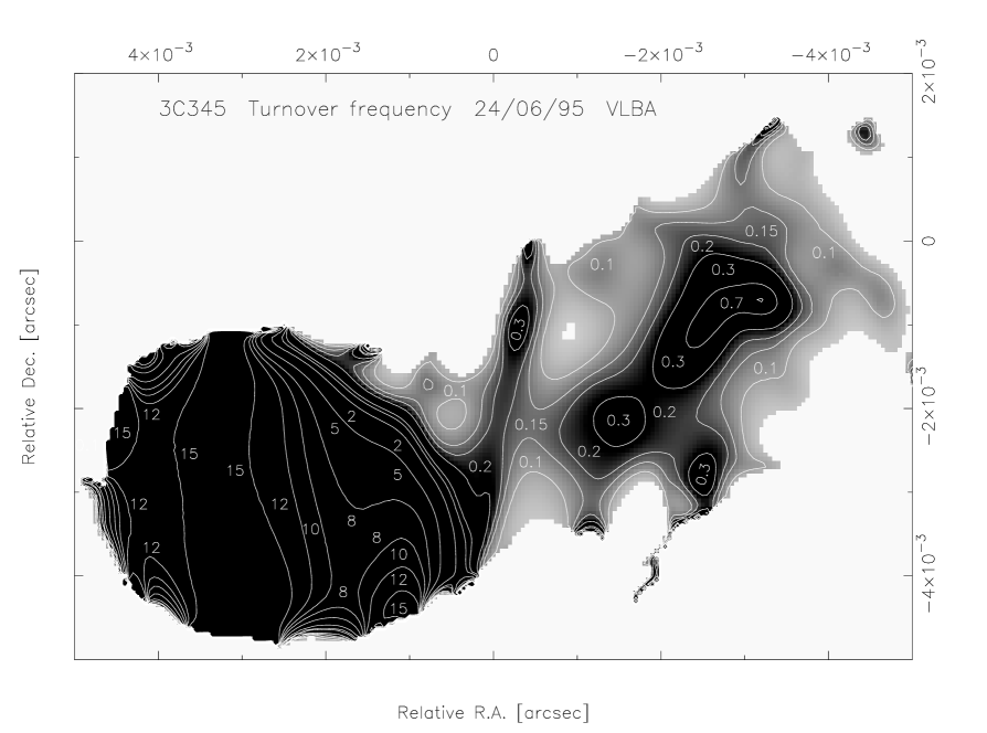
Figure 10: Turnover frequency distribution in the extended jet of 3C 345. The central region is saturated, for better representation of the turnover frequency variations in the jet. The contours are drawn at 0.1, 0.15, 0.2, 0.3, 0.7, 1, 2, 5, 8, 10, 12, and 15 GHz. All values below 5GHz should be regarded as upper limits.

6.1 Mapping the turnover frequency distribution in 3C 345

The blazar 3C 345 ($z=0.594$, Hewitt & Burbidge 1993) is a strongly variable core–jet type source with a compact core responsible for most of the source radio emission, and a curved, parsec–scale jet (Zensus et al. 1995) containing enhanced emission regions (bright components) travelling along curved trajectories, with speeds of up to 20 $c$ (Zensus et al. 1995). Synchrotron spectra of the core and the nearest bright components are often peaked around 10 GHz (Lobanov & Zensus 1998), and show a remarkable evolution. The emission from the core and the components is believed to be produced by condensations of highly–relativistic electron–positron plasma injected in the jet, and losing their energy first through the inverse–Compton mechanism (Kellermann & Paulini-Toth 1969; Unwin et al. 1997), and later on due to the synchrotron emission from adiabatically expanding relativistic shocks (Wardle et al. 1994; Zensus et al. 1995).

The turnover frequency procedure was applied to the multi–frequency VLBA observation of 3C 345 made on June 24, 1995. The source was observed at 5, 8.4, 15.4, and 22.2 GHz. At each frequency, there was roughly one 5 minute scan made every 20 minutes. After the correlation, the data were fringe–fitted and mapped in AIPS and DIFMAP (Shepherd 1993). The data were tapered at 150 M$\lambda$, and the maps were produced with a circular restoring beam of 1.2 mas in diameter. The core shift with respect to the reference frequency (22.2 GHz) was applied to the data at 5, 8.4, and 15.4 GHz. The magnitude of the core shift for the data at 15.4 GHz was determined from the fit $r_{\rm core}\propto\nu^{-1.04\pm 0.16}$, whereas for the data at 5 and 8.4 GHz the measured values were used (Lobanov 1998). The resulting maps are shown in Figure 9; the main characteristics of the maps are given in Table 3. Marked in the maps are the source core “D” and jet component “C7” which dominated the source emission at the epoch of observation.

The turnover frequency map produced from the VLBA maps shown in Figure 9 is presented in Figure 10. Figure 11 shows a map at 11 GHz obtained from the spectral fit to the combined VLBA data at 4 frequencies. One can see that the main features in the predicted 11 GHz image are consistent with the structures seen in the original VLBA maps.

Figure 11: Map of 3C 345 at 11 GHz obtained from the spectral fit. The restoring beam and contour levels are the same as in Figure 10. Spectral profiles in Figure 13 are taken along the horizontal line crossing the nuclear region of the source.

6.2 Nuclear region

In Figure 10, there are two regions of higher turnover frequency in the nucleus of 3C 345 oriented nearly transversely to the direction of the jet. These regions match the locations of the core and C7 fairly well. The increased turnover frequency may indicate that the emission is coming from a shocked plasma. The transverse extension is then consistent with strong shocks that are likely to be oriented almost perpendicularly to the jet direction. Figure 12 shows spectral profiles made along the horizontal line crossing the center of the core (horizontal line in Figure 11. The core and C7 are both visible in the turnover frequency profile. The turnover flux distribution is very smooth and peaks almost precisely at the center of the core. From the turnover frequency and turnover flux distributions, we can derive the profile of magnetic field in the central region using the relation (Cawthorne, 1991)

$$B(r)=C_{0}\nu_{\rm m}^{5}r^{4}S_{\rm m}^{-2},$$ (16)

where $C_{0}$ is the proportionality coefficient. $C_{0}$ can be determined empirically from the estimates of the absolute position ($r_{\rm core}\approx 5$ pc) and magnetic field ($B_{\rm core}\approx 0.3$ G) of the core at 22.2 GHz (Lobanov 1998):

$$C_{0}=B_{\rm core}S_{\rm m,core}^{2}\nu_{\rm m,core}^{-5}\approx 1.2\cdot 10^{-5}\,,$$ (17)

for the measured $S_{\rm m,core}=5.6$ Jy and $\nu_{\rm m,core}=15.1$ GHz. Equation 16 expresses the magnetic field strength due to the compression that the plasma has undergone during shock formation. Therefore, the magnetic field also depends on the strength of the underlying magnetic field in the location of the jet where the shock is formed. We postulate that the underlying magnetic field $B_{\rm amb}\propto r^{-m}$, and consider the cases, with $m=1$ and $m=2$. The jet is assumed to have a constant opening angle $\phi=2.4^{{}^{\circ}}$ (Lobanov 1998). For the magnetic field in an arbitrary pixel $p$, formula 16 yields

$$B_{\rm p}=C_{0}\nu_{\rm m,p}^{5}S_{\rm m,p}^{-2}(r_{\rm p}/r_{\rm core})^{4-m}\,\,\,\,[G],$$ (18)

In this formula, $\nu_{\rm m}$ is measured in GHz, $S_{\rm m}$ is in Jy, and $r$ is in parsecs. The resulting magnetic field profiles are plotted in Figure 12. The magnetic field rises sharply, close to the outer edge of C7. This can signify the amount of plasma compression in the shock. The increased magnetic field on the opposite side (particularly visible in the $B\propto r^{-2}$ profile) may reflect a larger electron plasma density near the jet origin. In the relativistic jets, the case $B\propto r^{-1}$ is expected to be more likely. A somewhat high value of the magnetic field in C7 ($B_{\rm C7}^{\rm max}\approx 8.5$ G) in this case may also be caused by possible errors in the estimates of the core magnetic field. However, the derived shape of the magnetic field profile is consistent with C7 being a strong shock embedded in the jet of 3C 345.

Figure 12: Profiles of turnover frequency, $\nu_{\rm m}$, turnover flux, $S_{\rm m}$, and magnetic field, $B(r)$, along the line $\Delta\delta=-3$ mas crossing the center of the core (horizontal line in Figure 12). The underlying magnetic field decreases along the jet as $r^{-m}$.

6.3 Extended jet

Almost everywhere in the extended jet shown in Figure 10, the turnover frequency is lower than 5 GHz, posing a problem for both the spectral fitting and assessing the results from the fits—we therefore resort to regarding all values of $\nu_{\rm m}\leq 5$ GHz as upper limits. Apparently, there are no strong shocks dominating the extended jet of 3C 345, or their turnover points may have evolved rapidly due to strong adiabatic cooling. Because the derived turnover frequencies are too low, we cannot make quantitative statements about the physical conditions in the extended jet. Observations at lower frequencies (1.6, 1.4, 0.6, 0.3 GHz) are required for a better understanding of the turnover frequency changes in these regions. With the available data, we can only make general comments about the gradients observed in the turnover frequency map. The bright patterns elongated along the jet ridge line may indicate the presence of an ultra-relativistic channel inside the jet (e.g. Sol et al 1989). The extended patterns seen in the jet at oblique angles to the ridge line resemble the patterns of Kelvin-Helmholtz instabilities (see Hardee et al. 1995, for the results from 3D simulations of the KH-instability driven jets). As has been noted above, the turnover frequency is exceptionally sensitive to the variations of plasma speed and density. Therefore, the observed patterns may reflect the velocity gradients and/or density gradients existing in the jet perturbed by the Kelvin-Helmholtz instability. However, the low frequency data are needed for making a better substantiated conclusion about the observed gradients.

7 Summary

In this paper, we have covered several methodological and scientific aspects of studying synchrotron spectrum of the parsec–scale regions in AGN. The main conclusions can be stated as follows:

1) We have discussed a technique that can be used for mapping the turnover frequency distribution and obtaining spectral information from multi–frequency VLBA data. A feasibility study shows that multi–frequency VLBA observations can be used for spectral imaging and continuous spectral fitting.

2) Multi–frequency VLBA observations made with up to 10 minute separations between the scans at each frequency can provide a satisfactory spatial sampling and image sensitivity for sufficiently bright sources with intermediate ($\sim 10$–15 mas) structures. The fractional errors from comparing the data at different frequencies should not exceed 10% for emission with SNR$\geq 7$, in this case.

4) A procedure for broadband synchrotron spectrum fitting has been introduced for mapping the distribution of spectral parameters of radio emission from parsec–scale jets. Corrections based on the local curvature of the fitted spectra are introduced, in order to compensate for the incomplete frequency coverage in cases where the true turnover frequency is outside of the range of observing frequencies.

5) From a 4–frequency VLBA observation of 3C 345, the first map of the turnover frequency distribution are produced. The maps indicate possible locations of the relativistic channel and strong shock fronts inside the jet. The magnetic field distribution derived from the turnover frequency and flux distributions is consistent with the plane shocks existing in the immediate vicinity of the source core. The extended emission appears to have a very low turnover frequency for which the existing data do not warrant a good estimate, limiting the conclusions to deducing certain information from the gradients of the turnover frequency which are visible in the extended jet. The observed gradients are consistent with the patterns of velocity distribution and density gradients typical for Kelvin–Helmholtz instabilities propagating in a relativistic jet. A more detailed study, with observations made at lower frequencies, is required for making conclusive statements about the nature of the observed gradients of the turnover frequency.

Appendix: Calculation of the local curvature of the fitted and theoretical spectral forms

Linear spectral forms

With the fitted polynomial coefficients $a_{0},...a_{3}$, we can write a linear form of the fit as:

$$S(\nu)=C_{0}\exp(\tau)\,,$$ (A1)

with $C_{0}=\exp(a_{0})$ and

$$\tau=\sum^{3}_{i=1}a_{i}(\ln\nu)^{i}\,.$$

And the derivatives used in (14) are given by the following formulae:

$$\frac{{\rm d}S}{{\rm d}\nu}=C_{0}\exp(\tau)\frac{{\rm d}\tau}{{\rm d}\nu}$$ (A2)

$$\frac{{\rm d}^{2}S}{{\rm d}{\nu}^{2}}=C_{0}\left[\exp(\tau)\frac{{\rm d}^{2}\tau}{{\rm d}{\nu}^{2}}+\exp(2\tau)\frac{{\rm d}\tau}{{\rm d}\nu}\right]$$ (A3)

$$\frac{{\rm d}\tau}{{\rm d}\nu}=\frac{1}{\nu}[a_{1}+2a_{2}\ln\nu+3a_{3}(\ln\nu)^{2}]$$ (A4)

$$\frac{{\rm d}^{2}\tau}{{\rm d}{\nu}^{2}}=-\frac{1}{\nu^{2}}[3a_{3}(\ln\nu)^{2}+(2a_{2}-6a_{3})\ln\nu+(a_{1}-2a_{2})]$$ (A5)

The power-law fit is given by:

$$S(\nu)=C_{1}\left(\frac{\nu}{\nu_{1}}\right)^{\alpha_{\rm t}}\left\{1-\exp\left[-\left(\frac{\nu}{\nu_{1}}\right)^{\alpha_{\rm o}-\alpha_{\rm t}}\right]\right\}\,,$$ (A6)

with the corresponding derivatives:

$$\frac{{\rm d}S}{{\rm d}\nu}=C_{1}\left[\nu^{\alpha_{\rm t}}\frac{{\rm d}\,f_{\nu}}{{\rm d}\nu}+\alpha_{\rm t}\nu^{(\alpha_{\rm t}-1)}f_{\nu}\right]$$ (A7)

$$\frac{{\rm d}^{2}S}{{\rm d}{\nu}^{2}} = C_{1}[\nu^{\alpha_{\rm t}}\frac{{\rm d}^{2}f_{\nu}}{{\rm d}\nu^{2}}+2\alpha_{\rm t}\nu^{(\alpha_{\rm t}-1)}\frac{{\rm d}\,f_{\nu}}{{\rm d}\nu}+$$

$$\quad\quad\quad\quad\quad\quad\quad\quad\quad\quad\quad\quad+(\alpha_{\rm t}-1)\alpha_{\rm t}f_{\nu}]$$

$$f_{\nu}=1-\exp\left[-\left(\frac{\nu}{\nu_{1}}\right)^{\lambda}\right]\,,\quad\lambda=\alpha_{\rm o}-\alpha_{\rm t}$$ (A9)

$$\frac{{\rm d}\,f_{\nu}}{{\rm d}\nu}=\frac{\lambda\nu^{\lambda-1}}{\nu_{1}^{\lambda}}\,\exp\left[-\left(\frac{\nu}{\nu_{1}}\right)^{\lambda}\right]$$ (A10)

$$\frac{{\rm d}^{2}f_{\nu}}{{\rm d}\nu^{2}}=\frac{\lambda\nu^{2\lambda-2}}{\nu_{1}^{2\lambda}}[(\lambda-1)\left(\frac{\nu_{1}}{\nu}\right)^{\lambda}-\lambda]\,\exp\left[-\left(\frac{\nu}{\nu_{1}}\right)^{\lambda}\right]$$ (A11)

Logarithmic spectral forms

Following the same considerations, the logarithmic form for the polynomial fit and its derivatives are:

$$S_{\rm log}(\nu)=\sum^{3}_{i=0}a_{i}(\ln\nu)^{i}$$ (A12)

$$\frac{{\rm d}S_{\rm log}}{{\rm d}(\ln\nu)}=a_{1}+2a_{2}\nu+3a_{3}\nu^{2}$$ (A13)

$$\frac{{\rm d}^{2}S_{\rm log}}{{\rm d}(\ln\nu)^{2}}=2a_{2}+6a_{3}\nu$$ (A14)

And for the power-law fit:

$$S_{\rm log}(\nu)=\ln C_{1}+\alpha_{\rm t}(\ln\nu-\ln\nu_{1})+\ln f_{\nu}$$ (A15)

$$\frac{{\rm d}\,f_{\nu}}{{\rm d}(\ln\nu)}=\lambda\left(\frac{\nu}{\nu_{1}}\right)^{\lambda}\,\exp\left[-\left(\frac{\nu}{\nu_{1}}\right)^{\lambda}\right]$$ (A16)

$$\frac{{\rm d}^{2}f}{{\rm d}(\ln\nu)^{2}}=\lambda^{2}\left(\frac{\nu}{\nu_{1}}\right)^{\lambda}\left[1-\left(\frac{\nu}{\nu_{1}}\right)^{\lambda}\right]\,\exp\left[-\left(\frac{\nu}{\nu_{1}}\right)^{\lambda}\right]$$ (A17)

$$\frac{{\rm d}S_{\rm log}}{{\rm d}(\ln\nu)}=\frac{1}{f_{\nu}}\frac{{\rm d}\,f_{\nu}}{{\rm d}(\ln\nu)}+\alpha_{\rm t}$$ (A18)

$$\frac{{\rm d}^{2}S_{\rm log}}{{\rm d}(\ln\nu)^{2}}=\frac{1}{f^{2}_{\nu}}\left[f_{\nu}\frac{{\rm d}^{2}f_{\nu}}{{\rm d}(\ln\nu)^{2}}-\left(\frac{{\rm d}\,f_{\nu}}{{\rm d}(\ln\nu)}\right)^{2}\right]$$ (A19)

References

- (1) Beasley, A.J. & Conway J.E. 1995, p. 291 in J.A. Zensus, P.J. Diamond, & P.J. Napier (eds.) 1995
- (2) Bridle, A.H. & Schwab, F.R. 1989, p. 247 in R.A. Perley, F.R. Schwab, & A.H. Bridle (eds.) 1989
- (3) Cawthorne, T.V. 1991, in Beams and Jets in Astrophysics, ed. P.A.Hughes (Cambridge: Cambridge University Press), 187
- (4) Crane, P.C. & Napier, P.J. 1989, p. 139 in R.A. Perley, F.R. Schwab, & A.H. Bridle (eds.) 1989
- (5) Cornwell, T. & Braun, R. 1989, p. 167 in R.A. Perley, F.R. Schwab, & A.H. Bridle (eds.) 1989
- (6) Cotton, D.W. 1995, p. 190 in J.A. Zensus, P.J. Diamond, & P.J. Napier (eds.) 1995
- (7) Ginzburg, V.L. & Syrovatskii, S. I. 1969, A&AAR, 7, 375
- (8) Hardee, P.E., Clarke, D.A., & Howell, P.A. 1995, ApJ, 441, 644
- (9) Hewitt, A., & Burbidge, G. 1993, ApJS, 87, 451
- (10) Kellermann, K.I., & Pauliny-Toth, I.K.K. 1969, ApJL, 155, L71
- (11) Königl, A. 1981, ApJ, 243, 700
- (12) Lobanov, A.P. 1996, Ph.D. Thesis (Socorro NM, USA: NMIMT)
- (13) Lobanov, A.P. 1998, A&A, 330, 79
- (14) Lobanov, A. P. & Zensus, J. A. 1998, ApJ, (submitted)
- (15) Marcaide, J.M., Shapiro, I.I., Corey, B.E., et al. 1985, A&A, 142, 71
- (16) Moran, J.M. & Dhawan, V. 1995, p. 161 in J.A. Zensus, P.J. Diamond, & P.J. Napier (eds.) 1995
- (17) Napier, P.J. 1995, p. 59 in J.A. Zensus, P.J. Diamond, & P.J. Napier (eds.) 1995
- (18) Pacholczyk, A.G. 1970, Radio Astrophysics (San Francisco: W.H.Freeman and Co.)
- (19) Pearson, T.J., 1991, BAAS, 23, 991
- (20) Pearson, T.J., Shepherd, M.C., Taylor, G.B., & Myers S. T., 1994, BAAS, 26, 1318
- (21) Perley, R.A., Schwab, F.R., & Bridle, A.H. (eds.) 1989, ASP. Conf. Series, Vol. 6, Synthesis Imaging in Radio Astronomy (San Francisco: ASP)
- (22) Rabaça, C.R., & Zensus, J.A. 1994, in Compact Extragalactic Radio Sources, eds. J.A.Zensus, & K.I.Kellermann (Green Bank: NRAO), 163
- (23) Romney, J.D. 1992, VLBA Specification Summary, (Socorro: NRAO)
- (24) Sol, H., Pelletier, H. & Asséo, E. 1989, MNRAS, 237, 411
- (25) Ternov, I.M. & Mikhailin V.V. 1986, Synchrotron emission: Theory and Experiment, (Moscow: Energoizdat)
- (26) Thompson, A.R., Moran, J.M., & Swenson, G.W.,Jr. 1986, Interferometry and Aperture Synthesis in Radio Astronomy, (New York: John Wiley & Sons)
- (27) Unwin, S.C., Wehrle, A.E., Lobanov, A.P., Zensus, J.A., Madejski, J.M., Aller, M.F., & Aller, H.D. 1997, ApJ, 480, 596
- (28) Walker, R.C. 1995, p. 133 in J.A. Zensus, P.J. Diamond, & P.J. Napier (eds.) 1995
- (29) Wardle, J.F.C., Cawthorne, T.V., Roberts, D.H., & Brown, L.F. 1994, ApJ, 437, 122
- (30) Wrobel, J.M. 1997, VLBA Observational Status Summary, p.7
- (31) Zensus J. A., Cohen M. H., Unwin S., 1995, ApJ, 443, 35
- (32) Zensus, J.A., Diamond, P.J., & Napier, P.J. (eds.) 1995, ASP Conf. Series, Vol.82, Very Long Baseline Interferometry and the VLBA (San Francisco: ASP)