Resonance in PSR B1257+12 Planetary System

Abstract

In this paper we present a new method that can be used for analysis of time of arrival of a pulsar pulses (TOAs). It is designated especially to detect quasi-periodic variations of TOAs. We apply our method to timing observations of PSR B1257+12 and demonstrate that using it it is possible to detect not only first harmonics of a periodic variations, but also the presence of a resonance effect. The resonance effect detected, independently of its physical origin, can appear only when there is a non-linear interaction between two periodic modes. The explanation of TOAs variations as an effect of the existence of planets is, till now, the only known and well justified. In this context, the existence of the resonance frequency in TOAs is the most significant signature of the gravitational interaction of planets.

1 Introduction

The first extra-solar planetary system was discovered by Wolszczan & Frail (1992) around a millisecond radio pulsar, PSR B1257+12. The three planets orbiting the pulsar have been indirectly deduced from the analysis of quasi-periodic changes in the times of arrival (TOAs) of pulses caused by the pulsar’s reflex motion around the center of mass of the system. In the analyses of this kind, it is particularly important to establish a reliable method of distinguishing planetary signatures from possible TOA variations of physically different origin. In the case of PSR B1257+12, it was possible to make this distinction and confirm the pulsar planets through the detection of mutual gravitational perturbations between planets B and C Wolszczan (1994), following predictions of the existence of this effect by Rasio et al. (1992), Malhotra (1992) (see also Malhotra (1993), Rasio et al. (1993) and Peale (1993)).

Practical methods of detection of the TOA variations caused by orbiting planets include direct fits of Keplerian orbits to the TOA or TOA residual data (Thorsett & Phillips, 1992; Lazio & Cordes, 1995, e.g.) and model–independent frequency domain approaches based on Fourier transform techniques Konacki & Maciejewski (1996); Bell et al. (1997). In fact, it appears that it is best to search for periodicities in TOAs (or post-fit TOA residuals left over from fits of the standard timing models) by examining periodograms of the data, and then refine the search by fitting orbits in the time domain using initial orbital parameters derived from a frequency domain analysis.

The presence of planets around a pulsar causes pulse TOA variations which, for planets moving in orbits with small eccentricities, have a quasi-periodic character and generate predictable, orbital element-dependent features in the spectra of TOA residuals. This has led Konacki & Maciejewski (1996) to devising a method of TOA residual analysis based on the idea of a successive elimination of periodic terms applied by Laskar (1992) in his frequency analysis of chaos in dynamical systems. The frequency analysis provides an efficient way to decompose a signal representing the TOA residual variations into its harmonic components and study them in an entirely model-independent manner. As shown in Konacki & Maciejewski (1996) this method works perfectly well under idealized conditions in which covariances among different parameters of the timing model are negligible.

In this paper, we present an improved scheme for the frequency analysis of pulsar timing observations in which a successive elimination of periodicities in TOAs is incorporated in the modelling process rather than being applied to the post-fit residuals. This makes the results obtained with our method less sensitive to the effect of significant covariances which may exist between various timing model parameters. We apply the frequency analysis to TOA measurements of the planet pulsar, PSR B1257+12, using a computer code developed to fit spectral timing models to data. We show that our method allows an easy detection of the fundamental orbital frequencies of planets A, B and C in the pulsar system and the first harmonics of the frequencies of planets B and C generated by eccentricities of the planetary orbits. Furthermore, by detecting the effect of perturbations between planets B and C, we demonstrate that the frequency analysis method represents a sensitive, model-independent tool to analyze nonlinear interactions between periodic modes of processes of various physical origins.

2 Development of the method

In the Fourier spectrum of a periodic process we detect the basic periodicity and some or all its harmonics. In the case of a quasi-periodic process, the Fourier spectrum contains a finite number of basic frequencies and their combinations with integer coefficients. A quasi-periodic signal represents a signature of the presence of interacting periodic processes. According to this description a real quasi-periodic function $S(t)$ of time $t$ can be written as a multiple Fourier series

$$S(t)=\sum_{\mbox{\scriptsize\bf k}}s_{\mbox{\scriptsize\bf k}}\exp[2\pi{\rm i}\langle\mbox{\bf k},\mbox{\bf f}\rangle t]=\sum_{\langle{\bf k,\bf f}\rangle\geq 0}a_{\mbox{\scriptsize\bf k}}\cos(2\pi\langle\mbox{\bf k},\mbox{\bf f}\rangle t)+b_{\mbox{\scriptsize\bf k}}\sin(2\pi\langle\mbox{\bf k},\mbox{\bf f}\rangle t),$$ (1)

where

$$\langle\mbox{\bf k},\mbox{\bf f}\rangle=\sum_{l=1}^{n}k_{l}f_{l},$$

$$\mbox{\bf f}=(f_{1},\ldots,f_{n}),\qquad\mbox{\bf k}=(k_{1},\ldots,k_{n}),$$

denote the vectors of basic frequencies, and the multi-index, respectively, and $s_{\mbox{\scriptsize\bf k}}$, $a_{\mbox{\scriptsize\bf k}}$, $b_{\mbox{\scriptsize\bf k}}$ are complex and real amplitudes corresponding to the frequency $\langle\mbox{\bf k},\mbox{\bf f}\rangle$. In (1) the first sum is taken over all possible multi-indices k with integer components $k_{i}$; the second sum is taken over all multi-indices k satisfying condition $\langle{\bf k,\bf f}\rangle\geq 0$. A finite sum (1) models a quasi-periodic signal of arbitrary origin with the amplitude of the signal corresponding to frequency $\langle\mbox{\bf k},\mbox{\bf f}\rangle$ expressed as:

$$A_{\mbox{\scriptsize\bf k}}=\sqrt{a_{\mbox{\scriptsize\bf k}}^{2}+b_{\mbox{\scriptsize\bf k}}^{2}}=2|s_{\mbox{\scriptsize\bf k}}|.$$

Let us consider a time series of observations $\{\psi_{i}\}_{i=1}^{N}$, representing a quasi-periodic process. If the influence of noise and sampling effects is negligible, the spectrum of $\{\psi_{i}\}_{i=1}^{N}$ will be characterized by a finite set of basic frequencies. In practice, any application of equation (1) to describe real data must properly account for the following facts: (a) data are unevenly sampled and contaminated by noise, (b) a possible range of signal amplitudes $[A_{min},A_{max}]$ can be very large, (c) periods corresponding to some harmonics present in the signal may be longer than the data span.

We approach the above problem using the following algorithm. Let $R_{0}=\{r_{l}^{0}\}_{l=1}^{N}$ denote a set of residuals obtained by fitting the standard pulsar model $\varphi(t)$ to observations. Using the least squares method, we fit a function $F_{(1)}(t)=\varphi(t)+a_{1}\cos(2\pi f_{1}t)+b_{1}\sin(2\pi f_{1}t)$ to the observations $\{\psi_{l}\}_{l=1}^{N}$. As the first approximation of $f_{1}$, we take a frequency corresponding to the maximum in the periodogram of $R_{0}$. For this purpose we use Lomb-Scargle periodogram Lomb (1976); Scargle (1982); Press et al. (1992).

After the $k$-th iteration, we have assembled a set of residuals $R_{k}=\{r_{l}^{(k)}\}_{l=1}^{N}$ defined as

$$r_{l}^{(k)}=\psi_{l}-F_{(k)}(t_{l}),\qquad l=1,\ldots,N,$$ (2)

where

$$F_{(k)}(t)=F_{(k-1)}(t)+a_{k}\cos(2\pi f_{k}t)+b_{k}\sin(2\pi f_{k}t),\quad F_{(0)}(t)\equiv\varphi(t),$$

and $t_{l}$, $l=1,\ldots,N$ denote observation times. Using the periodogram of $R_{k}$, we estimate $f_{k+1}$ and fit $F_{(k+1)}$ to the original data $\{\psi_{i}\}_{i=1}^{N}$. The whole process can be continued until a desired number of terms is obtained, or the final residuals fall below a predefined limit.

This algorithm represents an unconstrained frequency analysis, because we have implicitly assumed that all frequencies present in the signal are independent. If fewer basic frequencies are present in the signal, our algorithm can be modified to a constrained form. First, we examine a predefined number of basic frequencies $f_{1},\ldots,f_{k}$ to obtain residuals $R_{k}$. Then, we assume that the dominant frequency $f_{k+1}$ of the process is a predefined combination of $f_{1},\ldots,f_{k}$,

$$f_{k+1}=l_{1}f_{1}+\cdots+l_{k}f_{k},$$ (3)

where $l_{j}$, for $j=1,\ldots,k$ are integers and, as in the unconstrained case, we fit $F_{(k+1)}$ to the original data. Of course, in this case, $f_{k+1}$ is not a free parameter. If necessary, this process can be repeated for frequencies $f_{k+c}$, $c=1,2,\ldots$. In order to apply this algorithm, the coefficients of linear combinations (3) for all frequencies $f_{k+c}$, $c=1,2,\ldots$ have to be known in advance. In practice, it is conceivable that the signal amplitude at a constrained frequency (3) is greater than the amplitude at one or more basic frequencies. Consequently, an advance knowledge of the ordering of frequencies with respect to corresponding signal amplitudes is also necessary. This ordering can be easily derived from the unconstrained frequency analysis. We call this version of our algorithm the constrained frequency analysis.

Let us apply this approach to analyze TOAs of a pulsar with $N$ planets moving in orbits with small eccentricities. In the barycentric reference frame, with $z$-axis directed along the line of sight, changes in TOAs are proportional to the $z$-component of the pulsar radius vector. As stated by the KAM theorem Arnold (1978), for realistic planetary systems with weak interactions between planets, coordinates and velocities of planets are almost always quasi-periodic functions of time. Consequently, we assume that the motions of pulsar planets and hence the variations in a $z$-component of the pulsar vector are quasi-periodic. A presence of particular frequencies in the spectrum of TOAs is, in fact, predictable, namely, peaks with largest amplitudes should correspond to the basic (orbital) frequencies $f_{1},\ldots,f_{N}$ of the planets. Of course, the hierarchy of amplitudes depends on masses and semi-major axes of the planets. If eccentricities of orbits are greater than zero then the first harmonics of frequencies $2f_{1},\ldots,2f_{N}$ will have significant amplitudes. Ratios of spectral amplitudes at the fundamental frequencies and their first harmonics depend on the eccentricities of planetary orbits. If resonances are not present in a planetary system, the amplitude corresponding to frequency $l_{1}f_{1}+\cdots+l_{N}f_{N}$ decreases as $l=|l_{1}|+\cdots+|l_{N}|$ increases.

A simple resonance in a planetary system exists, if orbital periods of two planets $p$ and $q$ in the system are commensurate. Approximate resonance relationships, which represent most of the practical cases, are also treated as resonances. Thus, there is a simple orbital resonance $l_{p}:l_{q}$ between two planets $p$ and $q$ if frequency $f_{R}=l_{p}f_{p}+l_{q}f_{q}$ is small. In such a case, amplitudes corresponding to frequencies $f^{\pm}_{p}=f_{p}\pm f_{R}$ and $f^{\pm}_{q}=f_{q}\pm f_{R}$ are significant. The effect of resonance is caused by mutual interaction between planets, and thus its detecting in the spectra is a indirect confirmation of such interaction. Here we want to underline that the effect of the resonance does not manifest itself in observations by the presence of a significant harmonic term with the resonance frequency. The most characteristic appearance of a simple resonance is the presence of pairs of frequencies $f^{\pm}_{q}$ and $f^{\pm}_{p}$ located symmetrically around basic frequencies $f_{p}$ and $f_{q}$, respectively. Thus, the total effect of a resonance is a sum of four harmonic terms with frequencies $f^{\pm}_{q}$ and $f^{\pm}_{p}$.

3 Tests and Results

0bservations of PSR B1257+12 used to test the analysis method outlined above consist of 217 daily averaged TOAs covering the period in excess of four years. As shown by Wolszczan (1994), the observed TOA variations have a quasi-periodic character down to a $\sim$3 $\mu$s limit determined by noise.

The goal of our analysis was to identify all basic frequencies and their harmonics in the signal and, possibly to detect the characteristic signatures of a resonance effect.

3.1 Frequency Analysis

Our test analysis has been performed as follows. We generated fake TOAs for a pulsar orbited by three gravitationally interacting planets with orbital parameters chosen in such a way that the resonance had a period of 2059.2 days. These parameters were close to those given by Wolszczan (1994). The simulation covered a period of about eight and a half years. For the first half of the period fake TOAs were generated at the times of real observations, whereas for the second half TOAs were generated at the moments of real observations shifted by 4.22 years. A gaussian noise with the dispersion of 3$\mu$s was added to the synthetic TOAs.

In the first test, we performed a constrained frequency analysis of both data sets choosing three independent frequencies $f_{A}$, $f_{B}$, and $f_{C}$ corresponding to the orbital periods of the respective planets. As shown in Fig. 1, five different frequencies (ordered here by decreasing amplitudes) were identified in both data sets: $f_{1}=f_{C}$, $f_{2}=f_{B}$, $f_{3}=2f_{C}$, $f_{4}=2f_{B}$, $f_{5}=f_{A}$.

The unconstrained frequency analysis of the original and simulated TOAs detects peak frequencies listed in Table 2. We have examined a hypothesis that the detected peak frequencies $f_{3}$ and $f_{4}$ are indeed the first harmonics of $f_{1}$ and $f_{2}$ in the following way. Employing the frequency analysis, we fitted to data a quasi-periodic model representing a sum of five harmonic terms at frequencies: $f_{i}$, $i=1,\ldots 5$. In this process, frequencies $f_{3}$ and $f_{4}$ had fixed values inside an interval close to twice the basic planetary frequencies of planets C and B, respectively. After the fit, we calculated the values of two parameters $\alpha_{1}=f_{3}/f_{1}$ and $\alpha_{2}=f_{4}/f_{2}$ (so as $f_{3}=\alpha_{1}f_{1}$ and $f_{4}=\alpha_{2}f_{2}$) to obtain the weighted $\chi^{2}$ as a function of $(\alpha_{1},\alpha_{2})$. The results of this test (Fig. Resonance in PSR B1257+12 Planetary System) demonstrate that, within the limits set by a precision of the determination of frequencies $f_{1}$ and $f_{2}$ used to calculate $\alpha_{1}$ and $\alpha_{2}$, frequencies $f_{3}$ and $f_{4}$ are indeed the first harmonics of the fundamental frequencies of planets C and B.

3.2 Detection of the resonance effect

A direct frequency analysis of the original TOAs has failed to detect the effect of resonance. Since the rms TOA residual is $\sim$3$\mu$s compared to a predicted amplitude of the resonance term of about 1$\mu$s, this result is not surprising. However, there are four harmonic terms related to the resonance and their sum obviously has an amplitude that is higher than the noise level. Furthermore, the four frequencies related to the resonance lie symmetrically around the basic frequencies as is clearly visible in Fig. Resonance in PSR B1257+12 Planetary System. With this knowledge, and a fixed value of $f_{R}$, we fited to data a quasi-periodic model with frequencies: $f_{1}$, $f_{2}$, $f_{3}=2f_{1}$, $f_{4}=2f_{2}$, $f_{5}$, $f_{6,7}=f_{1}\pm f_{R}$, $f_{8,9}=f_{2}\pm f_{R}$. Varying $f_{R}$ we minimizeded a weighed $\chi^{2}$ as a function of $f_{R}$ to isolate any distinguished frequency $f_{R}$, whose presence might indicate the existence of a resonance effect between the observed TOA periodicities.

The result of this test for real data is shown in Fig. Resonance in PSR B1257+12 Planetary System. Although a position of the minimum, $f=6.9\times 10^{-4}$, does not coincide with that predicted by the theory, it is well defined indicating the detection of a real effect. The observed displacement of a $\chi^{2}$ minimum can be easily explained by the effect of a limited data span as shown in Fig. 5 which demonstrates that, with an increasing time coverage, the resonance frequency is determined with an increasing precision. Finally, to validate this test further, we repeated it with the data consisting of artificial TOAs modulated by Keplerian (i.e. noninteracting) planetary orbits. Clearly, in this case the minimum occurs at $f_{R}=0$, as expected in the absence of any resonance effect. Consequently, we confirm the presence of a resonance effect in the TOAs for PSR B1257+12, as originally demonstrated by Wolszczan (1994) using a time domain, real orbit analysis.

3.3 Keplerian elements of planets

Given the values of fundamental frequencies and amplitudes of their harmonics, orbital elements of planets can be calculated, assuming that they move in Keplerian orbits Konacki & Maciejewski (1996). Planetary masses can be calculated by assuming a pulsar mass to be $M_{\star}=1.4M_{\odot}$) and by setting orbital inclinations to 90^∘. We find that $e=0.0$, $m=0.0168\,M_{\oplus}$, $P=2189095$ (s) for planet A (only the fundamental frequency is significant so we assume that the planet’s eccentricity is zero), $e=0.0178$, $m=3.40\,M_{\oplus}$, $P=5748596$ (s) for planet B and $e=0.0229$, $m=2.83\,M_{\oplus}$, $P=8486539$ (s) for planet C. Finding $\omega$ and $T_{p}$ is also possible but it is more complicated. Clearly, these values are somewhat different from those given in Table 1(especially eccentricities). This is understandable, given that the frequency analysis-based model (constrained or unconstrained) and the one based on Keplerian orbits are not entirely equivalent. In the case of Keplerian orbits, frequencies and amplitudes are not independent parameters, while in the case of constrained frequency analysis only frequencies are constrained (as integer combinations of some fundamental frequencies) with all amplitudes remaining independent.

Clearly, the frequency analysis is not particularly convenient to determine Keplerian elements of planets. It is better to simply fit a suitable number of Keplerian orbits to observations. However, the frequency analysis procedure provides a good test of consistency with the results of fitting Keplerian orbits in time domain. It is encouraging to see that PSR B1257+12 planetary system does pass this test.

Table 1: PSR B1257+12 Planets Orbital Parameters

Parameter	A	B	C
$a\sin i$ (ms)	0.0035(6)	1.3106(6)	1.4121(6)
$e$	0.0	0.0182(9)	0.0264(9)
$T_{0}$ (JD)	2448754.3(7)	2448770.3(6)	2448784.4(6)
$P$ (s)	2189645(4000)	5748713(90)	8486447(180)
$f$ (deg)	0.0	249(3)	106(2)
$m$ ($\mbox{M}_{\oplus}$)	$0.015/\sin i_{A}$	$3.4/\sin i_{B}$	$2.8/\sin i_{C}$
$r$ (AU)	0.19	0.36	0.47

Table 2: Frequencies found in real and simulated observations

$f$	Real TOAs	Simulation
$f_{1}$	0.01018085	0.01001988
$f_{2}$	0.01502974	0.01478685
$f_{3}$	0.02035317	0.02003982
$f_{4}$	0.03004729	0.02957544
$f_{5}$	0.03947914	0.03943777
$2f_{1}-f_{3}$	8.53048$\cdot 10^{-6}$	-5.44713$\cdot 10^{-6}$
$2f_{2}-f_{4}$	1.21856$\cdot 10^{-5}$	-1.72562$\cdot 10^{-6}$

Frequency analysis of the real (left hand side) and simulated (right hand side) observations of PSR B1257+12. The top graphs (a and b) show TOA residuals for the real (a) and simulated (b) data after fitting the standard timing model. All other pictures are Lomb-Scargle normalized periodograms (LSNP) for which on the $x$-axis we have frequencies (in 1/day) and on the $y$-axis we have power units of LSNP (Press et al., 1992, p.577). A number near a pick in each periodogram is equal to the amplitude (in microseconds) of the component of the signal. In the second row, in LSNP of residuals $R_{0}$ for the real (c) and simulated (d) data we can see only fundamental frequencies of planets B and C. In the next step, in LSNP of $R_{2}$ we can see frequencies of second harmonics of planets B and C for both data sets (pictures e and f). Having subtracted them all from the signal (now, by fitting $F_{4}(t)$ to the data) we can see the fundamental frequency of the planet A (g and h). And finally, after additionaly subtracting the fundamental term of the planet A (by fitting $F_{5}(t)$ to the data), we see that in residuals $R_{5}$ of the real data (i) there is not a dominant pick, however one can see at least one of the peaks corresponding to the resonance frequencies $f_{B}\pm f_{R}$ and $f_{C}\pm f_{R}$ in LSNP of the fake data (j). In an idealized situation when the data densely cover the time domain, the respective periodogram looks like in Fig. 2.

LSNP of the last step of the frequency analysis of an idealized data set (one TOA per day without noise for the time span of two resonance periods). This figure corresponds to the pictures (i) and (j) in Fig. 1.

Test for the existence of the second harmonics of the planet fundamental frequencies. In the picture, $\alpha_{1}$ is the ratio of the fundamental frequency to the frequency $f_{3}$ (suspected to be the second harmonic) for the planet C and $\alpha_{2}$ is the corresponding value for the planet B. Contours correspond to confidence ellipses with marked confidence levels for $\Delta\chi^{2}(\alpha_{1},\alpha_{2})=\chi^{2}(\alpha_{1},\alpha_{2})-\chi^{2}_{0}$ where $\chi^{2}_{0}$ is the global minimum.

Detecting the resonance effect in the real data. In the picture, $f_{R}$ is a frequency in $1/$day. Confidence levels $1\sigma$, $2\sigma$, $3\sigma$ for $\Delta\chi^{2}(f_{R})=\chi^{2}(f_{R})-\chi^{2}_{0}$ where $\chi^{2}_{0}$ is the global minimum are shown. The minimum is well established around the frequency $f=6.9\times 10^{-3}$ that is shifted with respect to the resonance frequency $f_{r}=4.86\times 10^{-3}$ predicted by the theory. It results directly from the feature of the real data covering the time span shorter then the period of the resonance.

Detecting the resonace effect in the simulated TOAs of various origin. In the picture, $f_{R}$ is a frequency in $1/$day and $\Delta\chi^{2}(f_{R})$ is calculated as a departure from the global minimumu found for each case. (a) Test for the TOAs modulated by Keplerian planetary model. (b,c,d) Detecting the resonance for the fake TOAs resembling real observations but computed for different times spans: (b) data cover 0.75 of the resonance period, (c) data cover 1.0 of the resonance period, (d) data cover 2.0 of the resonance period. Increasing the time span allows to find the proper value of the resonance frequency.

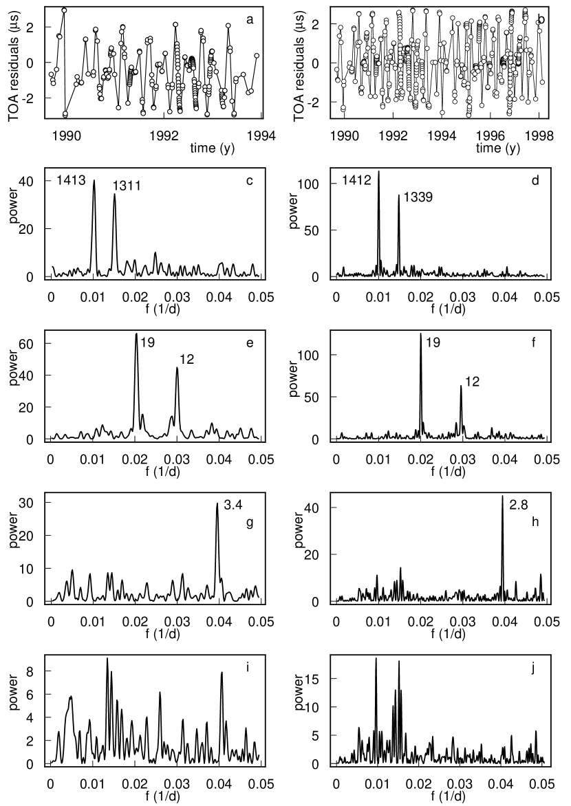
Figure 1:

Figure 2:

Figure 3:

Figure 4:

Figure 5:

Bibliography

- Arnold (1978) Arnold, V. I. 1978, Mathematical Methods of Classical Mechanics, Graduate Texts in Mathematics, Springer-Verlag, New York
- Bell et al. (1997) Bell, J. F., Bailes, M., Manchester, R. N., Lyne, A. G., Camilo, F. & Sandhu, J. S. 1997, MNRAS, 286, 463
- Konacki & Maciejewski (1996) Konacki, M. & Maciejewski, A. J. 1996, Icarus, 122, 347
- Lazio & Cordes (1995) Lazio, T. J. W. & Cordes, J. M. 1995, Mercury, march-april, 23
- Lomb (1976) Lomb, N. R. 1976, Ap&SS, 39, 447
- Malhotra (1992) Malhotra, R. 1992, Nature, 356, 583
- Malhotra (1993) Malhotra, R. 1993, in Planets around Pulsars, eds. J. A. Phillips, S. E. Thorsett & S. R. Kulkarni, vol. 36 of ASP Conference Series, pp. 89–106
- Peale (1993) Peale, S. J. 1993, AJ, 105, 1562
- Press et al. (1992) Press, W. H., Teukolsky, S. A., Vetterling, W. T. & Flannery, B. P. 1992, Numerical Recipes in C. The art of Scientific Computing, Cambridge University Press, New York, 2nd edn.
- Rasio et al. (1992) Rasio, F. A., Nicholson, P. D., Shapiro, S. L. & Teukolsky, S. A. 1992, Nature, 355, 325
- Rasio et al. (1993) Rasio, F. A., Nicholson, P. D., Shapiro, S. L. & Teukolsky, S. A. 1993, in Planets around Pulsars, eds. J. A. Phillips, S. E. Thorsett & S. R. Kulkarni, vol. 36 of ASP Conference Series, pp. 107–119
- Scargle (1982) Scargle, J. D. 1982, ApJ, 263, 835
- Thorsett & Phillips (1992) Thorsett, S. E. & Phillips, J. A. 1992, ApJL, 387, L69
- Wolszczan (1994) Wolszczan, A. 1994, Science, 264, 538
- Wolszczan & Frail (1992) Wolszczan, A. & Frail, D. A. 1992, Nature, 355, 145