Frequency Analysis of Reflex Velocities of Stars with Planets

Abstract

Since it has become possible to discovery planets orbiting nearby solar-type stars through very precise Doppler-shift measurements, the role of methods used to analyze such observations has grown significantly. The widely employed model-dependent approach based on the least-squares fit of the Keplerian motion to the radial-velocity variations can be, as we show, unsatisfactory. Thus, in this paper, we propose a new method that may be easily and successfully applied to the Doppler-shift measurements. This method allows us to analyze the data without assuming any specific model and yet to extract all significant features of the observations. This very simple idea, based on the subsequent subtraction of all harmonic components from the data, can be easily implemented. We show that our method can be used to analyze real 16 Cygni B Doppler-shift observations with a surprising but correct result which is substantially different from that based on the least-squares fit of a Keplerian orbit. Namely, using frequency analysis we show that with the current accuracy of this star’s observations it is not possible to determine the value of the orbital eccentricity which is claimed to be as high as 0.6.

1 Introduction

Recent improvements in the long-term precision of Doppler-shift measurements Butler et al. (1996) resulted in several spectacular detections of planetary companions to solar-type stars (for review see the paper of Marcy & Butler, 1997). As such discoveries supply indirect evidence of the existence of extra-solar planets, other explanations of observed radial-velocity variations appeared, e.g., stellar pulsations Gray (1997). The most recent results, however, show that only a planetary hypothesis is acceptable Marcy (1998); Gray (1998).

The usual procedure showing that there exists a planet around s star consits of a direct least-square fit of Keplerian model to the observations. It always gives certain values of orbital parameters and their formal errors. In the case of ‘good’ data this is the best and the quickest way to obtain relable results. However, in the case of spare data with big errors one has to prove that the least-squares method can be used and that the obtained parameter values and their errors are good estimates of the real values. This is a difficult and time consuming task. Without doubt, we have this situation with the Doppler observation of extra-solar planets. We present an analysis of this problem and we show that the eccentricity of the fitted orbit is a very sensitive parameter and, in some cases, its value and error given by the least-squares method are not correct.

The aim of this paper is to show how the mentioned problem can be solved in practice. Namely, we propose a method that can be very useful for analyzing radial-velocity variations. It is based on a simple idea involving the subsequent subtraction of periodic components from the data. This approach allows us to analyze the observations without assuming any specific model describing the system behavior (like Keplerian motion or stellar pulsations). After the determination of all significant components of the data, it remains to be decided which process is responsible for what we observe and whether it is possible to choose only one.

The plan of this paper is as follows. In Section 2 we analyse observations of 16 Cygni B and we explain why the standard least-squere fit does not give reliable estimates of parameters and their errors. In Section 3 we analyze analytically the Keplerian motion of the system ‘a star with one planet’ in order to learn how its motion modulates the observed star radial-velocities. We investigate mainly the spectral properties of the motion which are essential for our method. In Section 4 we develop a simple numerical technique which can be used to extract all the information we need to compare with the results from Section 3. In Section 5, we perform a numerical test of the method using simulated radial-velocity variations with the orbital parameters of 70 Vir Marcy & Butler (1996). In section 6, we discuss the application of the method to finding the eccentricity of 16 Cygni B Cochran et al. (1997).

2 Least-squares analysis of radial velocities of 16 Cygni B

In order to determine the quality and reliability of the least-squares fit of a Keplerian orbit to the radial velocity measurements of 16 Cygni B performed by Cochran et al. (1997) we analyzed the topology of the $\chi^{2}$ minimum on the $(a,e)$ plane, where $a$ is the semi-major axis and $e$ is the eccentricity. To this end, we used the real observations published in Cochran et al. (1997) and the Levenberg-Marquard method to solve the nonlinear least-squares problem (in our case a fit of a Keplerian orbit) which cannot be linearized (as this is the case for 16 Cygni B observations, as we show below). We took the necessary FORTRAN code from MINPACK library More et al. (1980). As the semi-major axis and the eccentricity are the most crucial parameters of the model, we compute the behavior of

$$\chi^{2}=\sum_{i}\frac{(v^{i}_{modeled}-v^{i}_{observed})^{2}}{\sigma_{i}^{2}}$$

on the $(e,a)$ plane. For a given point $(a,e)$ other parameters $(P,T_{p},\omega)$ are always chosen to correspond to the global minimum of $\chi^{2}$, i.e., for fixed values of parameters $(a,e)$ we make a series of fits with initial values of the elements $(P,T_{p},\omega)$ covering their whole range and we take the smallest value of $\chi^{2}$. In this way we get the behavior of $\chi^{2}$ on the $(e,a)$ plane, see Figure Frequency Analysis of Reflex Velocities of Stars with Planets. As one can see the confidence levels $1\sigma,2\sigma,3\sigma$ of the parameters $(e,a)$ bound a large region of the parameters’ plane. This shows that $e$ is very weakly determined with the data available for 16 Cygni B. At this point we make a well known but important remark. Namely, as one can see in Figure Frequency Analysis of Reflex Velocities of Stars with Planets, the confidence lines do not determine ellipses as it should be if we could use $1\sigma,2\sigma,3\sigma$ levels to determine the errors of $a$ and $e$ Press et al. (1992). It also means that the errors of the parameters obtained from the linearized (or not) least-squares fit cannot be treated as the correct estimates of the parameters’ accuracy. Thus, for example, the value 0.082 from the paper of Cochran et al. (1997) has little to do with the accuracy of the determined eccentricity. In fact, using nonlinear Levenberg-Marquard least-squares method we find a better solution for the same data of 16 Cygni B (this solution is marked with a filled square in Figure Frequency Analysis of Reflex Velocities of Stars with Planets; the filled star indicates the orbital solution found by Cochran et al. (1997)). One can compare the $\chi^{2}$ behavior with a very similar picture obtained by means of the bootstrap method Press et al. (1992), see Figure Frequency Analysis of Reflex Velocities of Stars with Planets. Clearly the distribution of $a$ and $e$ is not normal. Moreover, from this distribution we learn that any value of the eccentricity within the interval approximately $(0.25,1.0)$ is probable at the $3\sigma$ level.

To sum up, one can always use the least-squares method to obtain the orbital parameters. This method always gives a solution but sometimes the obtained parameters together with its errors have little to do with the real ones, whatever they are. However, the process of checking if the obtained result is correct is time consuming, and thus it seems resonable to find a simple method which can give the correct answer quickly. We address this problem in Sections 3 and 4.

3 Theoretical Background of Frequency Analysis

Let us assume that we have a planetary system consisting of a star and one planet. Choosing the reference frame placed in the center of mass of this system (barycentric system) with the $Z$-th axis directed from the observer, we can calculate the $Z$-th coordinate of the star from the following equation

$$Z_{\star}(t)=-\frac{m}{m_{\star}}Z(t),$$ (1)

where $m_{\star}$ is the mass of the star, $m$ is the mass of the planet and $Z$ is its $Z$-th coordinate. Next, because of the Keplerian motion of the system, we have

$$Z(t)=a\sin{i}\left(\sin\omega\left(\cos E-e\right)+\cos\omega\sqrt{1-e^{2}}\sin E\right),$$ (2)

where $a,i,\omega,e$ are Keplerian elements of the planet (semi-major axis, inclination, longitude of periastron and eccentricity) and $E$ is its eccentric anomaly that can be calculated from the Kepler equation

$$E-e\sin E=M,\qquad M=n(t-T_{p}),\qquad n=\frac{2\pi}{P},$$ (3)

where $M$ is the mean anomaly, $P$ is the orbital period of the planet and $T_{p}$ is the time of periastron. It was shown by Konacki & Maciejewski (1996) that function (1) can be expanded in the following series

$$Z_{\star}(t)=-\frac{m}{m_{\star}}\left(Z_{0}+\sum_{k=-\infty}^{k=+\infty}\!\!\!\!{}^{{}^{\prime}}\,Z_{k}{\rm e}^{{\rm i}kn(t-t_{0})}\right),$$ (4)

where

$$Z_{k}=\frac{1}{2k}\left\{C[J_{k-1}(ke)-J_{k+1}(ke)]+{\rm i}S[J_{k-1}(ke)+J_{k+1}(ke)]\right\}{\rm e}^{-{\rm i}knT_{p}},$$

and

$$Z_{0}=-\frac{3}{2}ea\sin i\sin\omega,\quad C=a\sin i\sin\omega,\quad S=-a\sqrt{1-{e}^{2}}\sin i\cos\omega.$$

In the above $J_{n}(z)$ is a Bessel function of argument $z$.

This expansion has a very important property—terms corresponding to successive harmonics have decreasing amplitudes. In this way, the term with the frequency $n$ has a larger amplitude than that with frequency $2n$, which has larger amplitude than that with frequency $3n$, etc. Generally, it is possible to prove the following inequality Konacki & Maciejewski (1996)

$${\cal A}_{k}(Z)=\frac{\left|Z_{k+1}\right|}{\left|Z_{k}\right|}=\frac{k}{k+1}\Psi_{k}(e,\omega)<1,$$ (5)

for each $e\in(0,1)$ and $\omega\in[0,2\pi)$; in (5) we denote

$$\Psi_{k}(e,\omega)=\sqrt{\frac{\beta^{2}\tan^{2}\omega[J_{k+1}^{\prime}((k+1)e)]^{2}+[J_{k+1}((k+1)e)]^{2}}{\beta^{2}\tan^{2}\omega[J_{k}^{\prime}(ke)]^{2}+[J_{k}(ke)]^{2}}},$$ (6)

and $\beta^{2}=e^{2}/(1-e^{2})$. When $e=0$ only the first term with frequency $n$ has a non-zero amplitude.

These considerations allow us to state the following: Keplerian motion of the planet orbiting a star leads to specific changes in the $Z$-th coordinate of a star. These changes have a very characteristic spectrum in which the term with frequency equal to the mean motion of the planet $n$ is dominant and amplitudes of subsequent harmonics (with frequencies $2n,3n,\dots$) decrease strictly monotonically.

The expansion of the Keplerian motion we show above can be easily applied to calculate the radial velocity of the star resulting from its motion in the system. Having the expansion of the $Z$-th coordinate of the star, we derive its radial-velocity by differentiating (4) with respect to time

$$v_{r}(t)=-\frac{{\rm d}Z_{\star}(t)}{{\rm d}t}=n{\frac{m}{m_{\star}}}\sum_{k=-\infty}^{k=+\infty}\!\!\!\!{}^{{}^{\prime}}\,{\rm i}kZ_{k}{{\rm e}^{{\rm i}kn(t-t_{0})}}.$$ (7)

As it can be easily noticed, the above expansion has the same feature as the expansion of the $Z$-th coordinate. In fact, the ratio ${{\cal A}_{k}(v_{r})}$ of two successive harmonics is always less than 1, since we have Konacki & Maciejewski (1996)

$${{\cal A}_{k}(v_{r})}=\frac{\left|Z_{k+1}(k+1)n\right|}{\left|Z_{k}kn\right|}=\frac{k+1}{k}{\cal A}_{k}(Z)=\Psi_{k}(e,\omega)<1.$$ (8)

Thus, all useful properties of the radial velocity expansion can be derived from that of the $Z$-th coordinate.

In summary, if we observe radial-velocity variations that are of planetary origin then in their spectra we will detect the basic frequency corresponding to the planet orbital period and its harmonics with monotonically decreasing amplitudes. The ratios of successive harmonics depend on the value of the eccentricity and the longitude of periastron. It means that in the case of a circular orbit we will be able to notice only one periodic term (which is obvious) and with increasing eccentricity the number of detectable harmonics will increase. Finally, we should mention that, because of the finite accuracy of our observations, we can only detect a few higher harmonics. Thus, from the observational point of view, expansion (7) is always finite and includes the basic term (corresponding to the planet orbital period) and a few of its harmonics.

Let us note that we can examine characteristic features of the spectra of other processes (e.g. stellar pulsations) and compare them with the expansion of Keplerian induced radial-velocity variations. Such information might be crucial for the proper interpretation of observations.

4 Numerical Realization of Frequency Analysis

Let ${\cal V}^{0}$ denote a set of radial velocities of a star obtained from the Doppler-shift measurements. Using the least-squares method, we fit the function $F_{1}(t)=A_{1}\sin(2\pi f_{1}(t-t_{0}))+B_{1}\sin(2\pi f_{1}(t-t_{0}))$ to the data. As the first approximation of $f_{1}$, we take the frequency corresponding to the maximum of the Lomb-Scargle periodogram of ${\cal V}^{0}$ Lomb (1976); Scargle (1982); Press et al. (1992).

At the $k$-th stage of this algorithm, we have a set of the residuals ${\cal V}^{k}$ obtained by fitting function $F_{k}$ to the original observations, where

$$F_{k}(t)=F_{k-1}(t)+A_{k}\sin(2\pi f_{k}(t-t_{0}))+B_{k}\cos(2\pi f_{k}(t-t_{0})).$$ (9)

This means that at the $k$-th stage of the algorithm we have the following model function $F_{k}(t)$:

$$F_{k}(t)=\sum_{j=1}^{k}A_{j}\sin(2\pi f_{j}(t-t_{0}))+B_{j}\cos(2\pi f_{j}(t-t_{0})).$$ (10)

Then, using the periodogram of ${\cal V}^{k}$, we approximate $f_{k+1}$, and we fit function $F_{k+1}$ to the original set of radial-velocities. These steps are repeated until the desired number of terms is obtained or until the final residuals are smaller than the assumed limit. We call the above algorithm unconstrained frequency analysis, as we assume that all frequencies we find are independent. However, we can modify our method to the constrained form. To this end, we assume that all terms have frequencies that are natural combinations of the chosen basic frequency $f_{b}$

$$f_{j}=jf_{b},\quad j=1,\ldots,k.$$ (11)

Thus the model we fit to the observations has the form

$$v_{r}(t)=\sum_{j=1}^{k}A_{j}\sin(2\pi jf_{b}(t-t_{0}))+B_{j}\cos(2\pi jf_{b}(t-t_{0})).$$ (12)

In this way parameters of the model are $f_{b},A_{j},B_{j}$ and not $f_{j},A_{j},B_{j}$; $j=1,\ldots,k$. We call this version of the algorithm the constrained frequency analysis.

Numerical tests of this method can be found in Konacki & Maciejewski (1996) and its successful applications to the PSR B1257+12 pulsar timing observations in Maciejewski & Konacki (1997); Konacki et al. (1998). In the next section we show how this method works on a simulated set of radial velocity measurements.

5 An Example - 70 Virginis

For the purposes of this example, we have chosen the orbital parameters of 70 Vir Marcy & Butler (1996). They are presented in Table 1 where we also present several periods and corresponding amplitudes calculated from expansion (7). For our tests, we computed data that are very similar in nature to the real observations. Thus we have 39 unevenly sampled radial-velocities. We also added 10 ms^-1 Gaussian noise resembling the real observational error.

In Figure Frequency Analysis of Reflex Velocities of Stars with Planets we present results from the unconstrained frequency analysis for the data described above. What can we learn about the planetary system from these results? First, we notice that the eccentricity of the orbit of 70 Vir is large since we are able to detect three periodic terms in the data. In fact, from the ratio of the amplitudes of the basic term to its first harmonic, we can precisely calculate the eccentricity (see Konacki & Maciejewski, 1996; Konacki et al., 1998).

Let us assume now that we do not know that these radial-velocity variations are of planetary origin. From the unconstrained frequency analysis for 70 Vir we find out that there are three periodic terms detectable, and, up to the accuracy of the method, they are all natural combinations of a certain basic frequency. This basic frequency corresponds to the term with the largest amplitude. It means that in fact, we see effects from the basic frequency and its two subsequent harmonics. Moreover, the ratio of their amplitudes resembles a process of planetary (Keplerian) origin. It is extremely unlikely that there are other reasonable processes that can produce such spectra and in this way mimic a planet. Thus, taking into account all the facts, the most natural answer would be that we observe radial-velocity variations induced by a planet in an eccentric orbit.

In summary, frequency analysis can supply us with strong constraints on the possible models of observed radial-velocity variations and verify the orbital solution obtained from a least-squares fit. We should also notice that we can apply the constrained frequency analysis as well; it usually results in a better fit and can be used to obtain better approximations of values of the amplitudes and basic frequency. Finally, one can compare this result with the behavior of $\chi^{2}$ in Figure Frequency Analysis of Reflex Velocities of Stars with Planets. The comparison shows that in many cases the frequency analysis will not be superior to the least-squares fit but will give an idependent insight into the data. Therefore, it is appropriate to use both methods while analyzing radial velocity measuerements, as the frequency analysis is numerically not demanding and has the capablility of confirming the least-squares’ findings.

We should also mention that it is possibible to interpret the observations in a different way which might be as well justified as the original assumption. Namely, it is possible to show that in some cases a planetary system consisting of two (or more) planets can be misinterpreted as one planet in a highly eccentric orbit and vice versa. This is easily understandable since from the frequency analysis we know that an eccentric orbit just produces a finite set of harmonics in the real data which subsequently might be interpreted in different manners. As there are some difficulties with the explanation of the existence of planets with highly eccentric orbits (see the paper of Marcy & Butler (1998) and reference therein for a discussion of this topic) and there is no obvious reason why the planets discovered around the Solar-type stars should be the only ones in their systems the above idea might be worth checking.

6 Frequency Analysis of 16 Cygni B observations

We applied the frequency analysis to real observations of 16 Cygni B. According to Cochran et al. (1997) the planet is believed to move in an highly eccentric orbit (e=0.634). We calculated theoretical amplitudes of the first harmonics of expansion (7), presented in Table 2. For calculation we took the orbital parameters obtained by means of the least squares method by Cochran et al. (1997). Comparing the values of amplitudes from Table 2 and the mean error of observations we concluded that we could detect at least the main frequency $n$ and its harmonic $2n$. We performed the frequency analysis of the real observations and we were only able to detect the basic frequency corresponding to the orbital period (see Figure Frequency Analysis of Reflex Velocities of Stars with Planets). After the subtraction of this term, there were no other dominant frequencies present in the data. Thus, our result obtained with the help of frequency analysis was inconsistent with result of Cochran et al. (1997) who reported the eccentricity 0.634 with uncertainty 0.082. This is, however, consistent with the results from Section 2. Stricly speaking, the frequency analysis reveals that the current quality of the data available for 16 Cygni B does not allow us to determine the eccentricity of the orbit due to the absence of any harmonics and confirms the findings based on the $\chi^{2}$ topology and the bootstrap method for these observations.

The final conclusion is that the real error of the eccentricity is much greater than that reported by the least-squares method, making the determination of the eccentricity of 16 Cygni B almost impossible. This fact can be easily derived from the frequency analysis. The absence of any harmonics just indicates that the eccentricity must remain undetermined. With the frequency analysis one gets this correct result without the time consuming $\chi^{2}$ map or the bootstrap method.

7 Conclusions

In this paper we have shown that results obtained from least-squares fits of Keplerian orbits to real Doppler-shift measurements may lead to incorrect interpretations. Specifically, they may give unrealistic or even entirely false values of parameters and their uncertainities. In order to solve these problems we have proposed a new method, frequency analysis, which efficiently provides an independent test of the reliability of determined orbital parameters. This method may deliver a substantial revision of the current values of planets’ high eccentricities that are essential for our understanding of the formation and evolution of planetary systems. It might even lead to hints that some of the observed high eccentric planets are in fact planetary systems consisting of more than one planet or at least provide an independent point of view on the same data. These facts, together with the ease of applicability of frequency analysis, make our method worth trying on future observations if not for the data already gathered.

$\chi^{2}$ map on the plane $(e,a)$ of the real data of 16 Cygni B. The filled square indicates the global minimum that is different than the orbital solution found by Cochran et al. (1997) denoted by the filled star. The significance levels ”$1\sigma$”, ”$2\sigma$” and ”$3\sigma$” are presented.

Bootstrap estimation of the distribution of $(e,a)$ based on the sample consisting of $10^{4}$ synthetic sets of data (left). Distribution of $e$ (right, top) and $a$ (right, bottom) calculated from the same sample. The distributions for both parameters are clearly not normal.

Unconstrained frequency analysis of the fake reflex velocity of 70 Vir. The simulated data consist of 39 points from 1988 to 1996.25, 10 ms${}^{-}1$ Gaussian noise was added. a,b,c,d: Subsequent steps of the frequency analysis. Found periods and their amplitudes are presented. Numbers in parentheses are $3\sigma$ uncertainties of the parameters. There are three detectable periodicities in the data.

$\chi^{2}$ map on the plane $(e,a)$ of the fake data of 70 Virginis. The filled square indicates the global minimum found and the star indicates the parameters assumed while calculating the fake data. The significance level $3\sigma$ is presented.

Unconstrained frequency analysis of the real reflex velocity of 16 Cygni B. The data taken from the paper of Cochran et al. (1997) consist of 70 points from about 1988 to 1997. a,b: Two subsequent steps of the frequency analysis. As one can see, there is only one periodic term detectable (a) corresponding to the planetary period of about 800 days. After subtracting this periodicity there are no significant peaks in the data present. Solid and dash-dotted line correspond to 90 an 50 percent significance levels, respectively.

Table 1: Orbital and Theoretical Frequency Analysis Parameters of 70 Vir

70 Vir
$P$ (days)	116.67	$k=1$	$P1=116^{\mbox{d}}.67$	$A_{P1}=261.36\mbox{ ms}^{-1}$
$T_{p}$ (JD)	2448990.403	$k=2$	$P2=58^{\mbox{d}}.335$	$A_{P2}=101.08\mbox{ ms}^{-1}$
$e$	0.40	$k=3$	$P3=38^{\mbox{d}}.89$	$A_{P3}=43.83\mbox{ ms}^{-1}$
$\omega$ (deg)	2.1	$k=4$	$P4=29^{\mbox{d}}.1675$	$A_{P4}=19.99\mbox{ ms}^{-1}$
$a_{1}\sin i$ (AU)	0.00312	$k=5$	$P5=23^{\mbox{d}}.334$	$A_{P5}=9.39\mbox{ ms}^{-1}$

Table 2: Orbital and Theoretical Frequency Analysis Parameters of 16 Cyg B

16 Cyg B
$P$ (days)	800.8	$k=1$	$P1=800^{\mbox{d}}.8$	$A_{P1}=28.89\mbox{ ms}^{-1}$
$T_{p}$ (JD)	2448935.3	$k=2$	$P2=400^{\mbox{d}}.4$	$A_{P2}=16.14\mbox{ ms}^{-1}$
$e$	0.634	$k=3$	$P3=200^{\mbox{d}}.2$	$A_{P3}=10.23\mbox{ ms}^{-1}$
$\omega$ (deg)	83.2
$K$ ($\mbox{ms}^{-1}$)	43.9

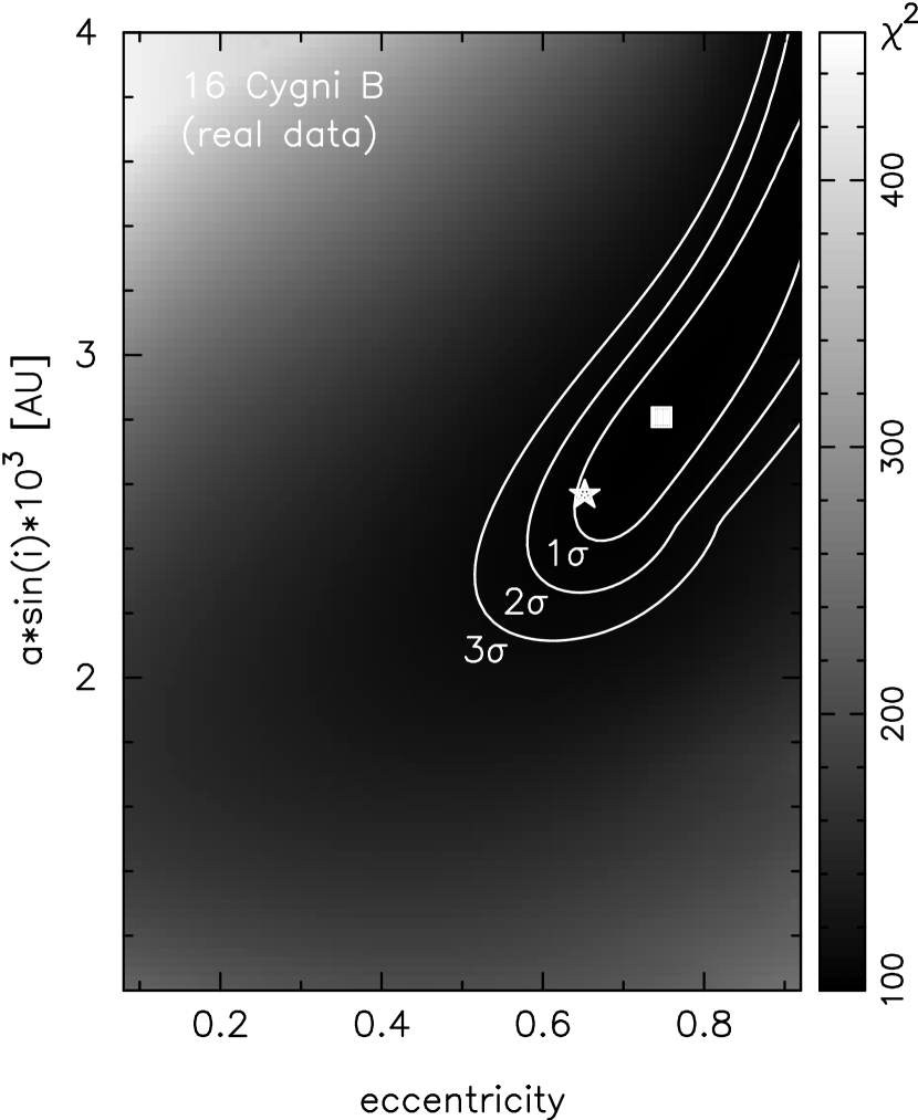
Figure 1:

Figure 2:

Figure 3:

Figure 4:

Figure 5:

Bibliography

- Butler et al. (1996) Butler R. P., Marcy G. W., Williams E., McCarthy C., Dosanjh P., Vogt S. S., 1996, PASP, 108, 500–509.
- Cochran et al. (1997) Cochran W. D., Hatzes A. P., Butler R. P., Marcy G. W., 1997, ApJ, 483, 457–463.
- Gray (1997) Gray D. F., 1997, Nature, 385, 795–796.
- Gray (1998) Gray D. F., 1998, Nature, 391, 153–154.
- Konacki & Maciejewski (1996) Konacki M., Maciejewski A. J., 1996, Icarus, 122, 347–358.
- Konacki et al. (1998) Konacki M., Maciejewski A. J., Wolszczan A., 1998, submitted to ApJ.
- Lomb (1976) Lomb N. R., 1976, Ap&SS, 39, 447–462.
- Maciejewski & Konacki (1997) Maciejewski A. J., Konacki M., 1997, in D. Maoz, A. Sternberg, E. Leibowitz, eds, Astronomical Time Series, p. 227–230.
- Marcy (1998) Marcy G., 1998, Nature, 391, 127–127.
- Marcy & Butler (1996) Marcy G. W., Butler R. P., 1996, ApJ, 464, L147–L151.
- Marcy & Butler (1997) Marcy G. W., Butler R. P., 1997. to appear in the Proceedings of The Tenth Cambridge Workshop on Cool Stars, Stellar Systems and the Sun.
- Marcy & Butler (1998) Marcy G. W., Butler R. P., 1998. to appear in the Proceedings of the Workshop on Brown Dwarfs and Extrasolar Planets.
- More et al. (1980) More J. J., Garbow B. S., Hillstrom K. E., 1980, National Laboratory Report ANL-80-74.
- Press et al. (1992) Press W. H., Teukolsky S. A., Vetterling W. T., Flannery B. P., 1992. Numerical Recipes in C. The art of Scientific Computing. Cambridge University Press, New York, second edition.
- Scargle (1982) Scargle J. D., 1982, ApJ, 263, 835–853.