Large scale structure formation in mixed dark matter models with a cosmological constant

Abstract

We study linear power spectra and formation of large scale structures in flat cosmological models with $\Lambda\geq 0$ and cold plus hot dark matter components. We refer to these models as mixed $\Lambda$ models (MLM). The hot component consists of massive neutrinos with cosmological density $\Omega_{H}$ and number of neutrino species as a free parameter. The linearized Einstein-Boltzmann equations for the evolution of the metric and density perturbations are integrated for a set of values of the cosmological parameters. We study MLM models with present matter density in the range $0.25\leq\Omega_{M}\leq 1$, dimensionless Hubble constant $0.4\leq h\leq 0.7$ and the hot dark matter content with a ratio within the limits $0\leq\Omega_{H}/\Omega_{M}\leq 0.3$. For all the considered models we assume a scale-invariant primeval spectrum.

The density weighted final linear power spectra are normalized to the four year COBE data and have been used to constrain the parameter space by a comparison of linear predictions with the current observational data on large scales. The consistency of MLM predictions with the observable data set is best obtained for models with one species of massive neutrinos and $\Omega_{H}/\Omega_{M}\leq 0.2$. Of the considered linear tests the strongest constraints on $\Omega_{M}$ that we obtain arise by comparing the cluster X-ray temperature function with that observed at the present epoch. Consistency with the estimated cluster abundance can be achieved for COBE normalized MLM models with $\Omega_{H}/\Omega_{M}\leq 0.2$ and $0.45\leq\Omega_{M}\leq 0.75$ for $h=0.5$. If $h=0.7$ then $0.3\leq\Omega_{M}\leq 0.5$. These constraints are at $1\sigma$ level and standard MDM models are clearly ruled out.

We note that the range of allowed values for $\Omega_{M}$, that we obtain for MLM models from linear analysis, is also approximately the same range that is needed in order to consistently satisfy a variety of independent observational constraints.

1 Introduction

In the standard framework of gravitational instability theory present day structures must have been formed through the growth of small inhomogeneities from an initial random Gaussian density field present at very early epochs, with a scale-invariant Harrison-Zel’dovich spectrum. Clustering analysis of the large scale structure in the Universe has been improved in recent years by observations of the spatial distribution of galaxies and cluster of galaxies, as well as cosmic microwave background (CMB) anisotropies. Thus any theory that wants to fit the observed large scale clustering must be consistent with a set of constraints over more than three decades in length: from galaxy correlation ($\sim 1{h}^{-1}Mpc$, $H_{0}=100hKmsec^{-1}Mpc^{-1}$ ) up to the quadrupole CMB anisotropies detected by COBE ($\sim 3000{h}^{-1}Mpc$, [Smoot et al. 1992]).

In the standard FRW metric the fundamental background cosmological parameters are related by a mutual relation. It is also understood that for these parameters (the present matter density $\Omega_{M}$, the value of the Hubble constant $H_{0}$ and the age of the universe $t_{0}$) the range of values allowed by observations must be consistent with their FRW relation. If we adopt the standard inflation theory we shall assume that the total energy density in the Universe is equal to the critical density ($\Omega_{0}=1$). On the other hand, observations and theoretical predictions suggest that the amount of baryon density must be small ($\Omega_{b}\sim 0.05{(h/0.5)}^{-2}$, [Walker et al. 1991], [Copi, Schramm & Turner 1995]). A much larger contribution to the matter density must be of non-baryonic nature. This is so-called dark matter (DM) problem and it has observational support from dynamical estimates ($\Omega_{M}\sim{0.2-0.3}$, [Bahcall 1996] and references cited therein). It must be stressed that there is not yet a firm evidence for $\Omega_{M}=1$, this value for $\Omega_{M}$ being required by the inflationary paradigm. The simplest possible model of DM is the one in which the universe is dynamically dominated by a single massive collisionless particle. The most popular DM candidates are collisionless massive particles, which decoupled from cosmological plasma either when being relativistic (DM particles like massive neutrinos – Hot DM) or non-relativistic (hypothetical massive particles – Cold DM).

The simplest model is CDM, where the power spectrum of the perturbations depends on a single parameter, the present cold density $\Omega_{C}$. Historically the first model to be considered was a neutrino with a non-zero rest mass HDM ([Bond & Szalay 1983]; [Zakharov 1979]). The HDM model was soon rejected because numerical simulations ( [White, Frenk & Davis 1983]) produced nonlinear structures too late to be in agreement with QSO existence. The standard CDM model (SCDM) has been analysed in considerable details ([Davis et al. 1985]; [Davis & Efstathiou 1988] and references cited therein). It can match galaxy clustering ($\raise-2.0pt\hbox{\hbox to0.0pt{\hbox{$\sim$}\hss}\raise 5.0pt\hbox{$<$}\ }10{h}^{-1}Mpc$) with a bias parameter $b_{g}\raise-2.0pt\hbox{\hbox to0.0pt{\hbox{$\sim$}\hss}\raise 5.0pt\hbox{$>$}\ }2$, although it lacks of sufficient power on large scales. The SCDM model however became seriously inconsistent with clustering data after the COBE detection of a quadrupole anisotropy in the CMB ([Smoot et al. 1992]). When the power spectrum of the model is normalized to the COBE data SCDM models have unavoidable difficulties ([White, Efstathiou & Frenk 1993a]; [Olivier et al. 1993]; [Mo, Jing & Borner 1993]; Jing & Valdarnini 1993; Dalton et al. 1991 ; Baugh & Efstathiou 1994).

The Mixed Dark Matter models (MDM) was at first proposed and discussed in a few papers (Fang, Xiang & Li 1984; Shafi & Stecker 1984; Achilli, Occhionero & Scaramella 1985; Valdarnini & Bonometto 1985) as an example to overcome the standard Hot Dark Matter (SHDM). Later, SMDM models were readressed again ([Holtzman 1989]; [Van Dalen & Schaefer 1992]). Finally, it was proposed that a certain mixture proportion of about $30/70\%$ for the Hot/Cold DM ([Schaefer & Shafi 1992]; [Davis, Summers & Schlegel 1992]; [Taylor & Rowan-Robinson 1992]; Klypin et al. 1993; Pogosyan & Starobinsky 1993) as a DM model satisfying a wide body of observational data for clustering ( distributions of galaxies, galaxy clusters, quasars, Ly-$\alpha$ systems, etc.) on typical scales $\leq l_{LS}\sim 100-150{h}^{-1}Mpc$ and with an Harrison-Zeldovich spectrum of the primordial cosmological perturbations on scales $>l_{LS}$. Because of the changes introduced into the power spectrum by neutrino clustering, for SMDM models it was shown the possibility to reconcile the evidence of high coherent velocity flows on large scales ($\sim 50{h}^{-1}Mpc$ ) with the moderate galactic pair velocities on megaparsec scales ([Klypin et al. 1993]). For the cluster correlation function ( [Holtzman & Primack 1993]; [Jing et al. 1993]; [Klypin & Rhee 1993]) the two-point function for SMDM models appears to be consistent with data for $R\raise-2.0pt\hbox{\hbox to0.0pt{\hbox{$\sim$}\hss}\raise 5.0pt\hbox{$>$}\ }20-30h^{-1}Mpc$ ( on the contrary to what found for CDM ).

Analytical approximations for the present epoch transfer functions are given by Holtzmann (1989); Pogosyan & Starobinsky (1995); Ma (1996); Eisenstein & Hu (1997). Early numerical simulations have considered $\Omega_{H}=0.3$, we will use the notation $H$ for massive neutrinos, but this model does not produce Ly-$\alpha$ systems as much as observed ([Mo & Miralda-Escude 1994]). For this reason a value of $\Omega_{H}\raise-2.0pt\hbox{\hbox to0.0pt{\hbox{$\sim$}\hss}\raise 5.0pt\hbox{$<$}\ }0.2$ results in a better fit ([Klypin et al. 1995]; [Ma & Bertschinger 1994]). In comparison with SCDM or SHDM, MDM models are more complicated, we have the choice of two independent parameters : the ratio $\Omega_{H}/\Omega_{C}$ and $m_{H}$ ( if one allows for more than one species of massive neutrinos). The spectral index $n$ of the post-inflationary spectrum is taken $n=1$. It is possible to consider also the role of gravitational waves, which can change significally the normalization of the spectrum and the formation of structures (e.g., [Ma 1996] ).

It must be stressed that SMDM models are in difficulty with the present upper limits on the age of the Universe: if we assume $h=0.5$ and the age of globular clusters greater than $15Gyr$, in the case of a flat FRW model the needed value of $\Omega_{M}$ is $\leq 0.6$. The other difficulties are connected with later galaxy and quasar formation ([Pogosyan & Starobinsky 1995]; [Cen & Ostriker 1994]). Another difficulty for SMDM models is that when the power spectra are normalized to the COBE 4-yr data the linear theory overpredicits the observed cluster abundances. The estimated uncertainties in the normalization and linear calculations can hardly fit the cluster number density within present data error bars. The difficulty can be reduced if one removes the constraint of a scale invariant spectra and introduces a small tilt ( $n\simeq 0.8-0.9$, [Ma 1996]).

In alternative to MDM models spatially flat low density models with a positive cosmological constant are considered to be a viable generalization of SCDM after COBE. These models are termed $\Lambda$CDM and were considered even before the quadrupole detection ([Peebles 1984] and references therein). There are two main reason to consider $\Lambda$CDM models as an alternative to MDM: the present lower limit on the age of the Universe and the baryon fraction in galaxy clusters.

Current uncertainties for the age of globular clusters give $t_{0}=15\pm 2Gyr$ ([Chaboyer et al. 1996]). If one takes a lower limits $t_{0}\geq 13Gyr$ then in the $\Omega_{M}=1$ case the maximum value for $h$ is $0.5$. This value is below the range allowed by recent HST measurement : $h=0.7\pm.1$ ([Freedman et al. 1994]; [Reiss, Kirshner & Press 1995]). The introduction of a positive cosmological constant allows $h$ to be higher for a fixed age $t_{0}$ than in $\Omega_{M}=1$. The other reason to consider $\Lambda$CDM model is from X-ray observations of galaxy clusters. If clusters are a representative sample of the matter content in the Universe, then their baryons/total matter ratio should not be different from what expected from standard nucleosynthesis ([White et al. 1993b]). For $h\raise-2.0pt\hbox{\hbox to0.0pt{\hbox{$\sim$}\hss}\raise 5.0pt\hbox{$>$}\ }0.5$ this is achieved if $\Omega_{M}\raise-2.0pt\hbox{\hbox to0.0pt{\hbox{$\sim$}\hss}\raise 5.0pt\hbox{$<$}\ }0.35\pm 0.2$. Quite interestingly this range is close to that obtained from dynamical estimates. After COBE detection of the quadrupole anisotropy $\Lambda$CDM models have been further considered (Kofman, Gnedin & Bahcall 1993; Klypin, Primack & Holtzman 1996; Liddle et al. 1996a; Liddle et al. 1996b). They can fit several constraints on large scales ($k\raise-2.0pt\hbox{\hbox to0.0pt{\hbox{$\sim$}\hss}\raise 5.0pt\hbox{$<$}\ }1{h}^{-1}{Mpc}^{-1}$, [Liddle et al. 1996b]), but small scales clustering it is excess ([Klypin, Primack & Holtzman 1996]) by a factor $\approx 2-3$ when compared to estimates from galaxy catalogs, so this is a difficulty of the model which can be solved with the introduction of an antibias of small scales. A possibility which seems unplausible ([Primack & Klypin 1996]).

These difficulties have suggested that consistency with present data can be achieved for standard DM models with the introduction of one extra parameter. Possible variants are two species of massive neutrinos ( Primack 1997 ), or a tilt of the primordial spectrum ( Cole et al. 1997 ).

The main aim of this paper is to consider an alternative possibility , that is MDM models with $n=1$ and a non-zero cosmological constant (MLM). These models have in fact the following free parameters : $\Omega_{H}/\Omega_{M}$, $\Omega_{\Lambda}$ and the number of species of massive neutrinos. If one considers one species of massive neutrinos, then MLM are on the same foot of the previous alternatives, the main advantage being that they retain the inflation paradigm and a scale-invariant initial spectrum.

In order to study these models we have numerically integrated forward in time the linearized Einstein-Boltzmann equations for the evolution of the metric and density perturbations. The final power spectra have been normalized according to the four year COBE data ([Bunn & White 1997]). We have then used linear perturbation theory to find the parameters for which MLM models are consistent with a variety of current observational constraints on large scales (power spectrum, cluster-cluster correlations, bulk velocities, cluster abundance). In order to make comparison with observations we will consider the following set of parameter space: $\Omega_{\Lambda}=0,0.31,0.45,0.65,0.74$; $\Omega_{H}/\Omega_{M}=0.1,0.2,0.3$; number of massive and massless neutrinos $\beta_{H}=2,4,6$ and $\beta_{\nu}=0,2,4,6$ ( here $\beta$ is the sum of spin states ). In some cases we considered a number of neutrinos species greater than three, this possibility being of no physical relevance, we ran these models for studying how different numbers of massive and massless particles would change the spectra evolution. Our final analysis will be restricted to one massive neutrino. The fifth parameter is $h$ ($h=0.4,0.5,0.63,0.7$).

The outline of the paper is as follows: in Section 2 we will present our model description and equations describing the linear perturbations in MLM models. In Section 3 we will study the power spectra dependence on model parameters using COBE 4-year data normalization. In Section 4 some linear tests are given for MLM models, including our results for the cluster mass and temperature function. Our conclusions are given in Section 5.

2 Theoretical framework

2.1 Equations and method

We have studied the evolution of density perturbations in a flat Friedmann cosmology. In our models the present total density in critical units is $\Omega_{0}=\Omega_{C}+\Omega_{H}+\Omega_{\Lambda}=1\equiv\Omega_{M}+\Omega_{\Lambda}$. The notation $H$ means massive neutrinos, $C$ cold dark matter and $\Omega_{\Lambda}=\Lambda/(3H_{0}^{2})$.

In our integrations we have followed numerically the time evolution of the linearized Einstein-Boltzmann equations for the metric and adiabatic density perturbations. We have considered scalar modes only and treated the perturbations for the following particle species : cold, massive and massless neutrinos ($\nu$), photons. We treat baryons and radiation as a single ideal fluid. We have assumed that all collisionless particles were decoupled from radiation before the beginning of our computation. In a collisionless medium the pressure anisotropy is different from zero and the equations for density contrast and velocity are not sufficient to describe the perturbations in $H$ and $\nu$ particles. Collisionless components must be described by the Boltzmann-Vlasov equation. The density contrast, flux velocity and pressure anisotropy are given by the moments of the perturbed distribution functions.

The set of equations for fluid and collisionless media, with the Einstein equations for metric perturbations, describes the evolution of density perturbations in MLM models. The method of numerical solution of this system is described in Valdarnini & Bonometto (1985), and we refer to this paper for more details. The generalization of the equations to include a non-zero cosmological constant is straightforward.

Our numerical calculation is done for the following range of perturbation masses : from $M=10^{20}M_{\odot}$ down to $M=10^{11}M_{\odot}$. The integrations start at the initial redshift $z_{i}=10^{9}$ and stop at the final epoch $z_{f}=5$. Because of the large region of parameter space that we have spanned with our integrations, and the computational resources we had available, we have decided to stop the numerical integrations at a final epoch $z_{f}>0$. As a compromise between computing budget and the accuracy needed to evaluate observational linear variables at the present epoch we chose $z_{f}=5.$

The initial conditions for our linear computations are given by the Harrison-Zeldovich ( $n=1$ ) spectrum of density fluctuations:

$$\mid\delta_{C}(k)\mid^{2}=A_{i}k,$$

where $k$ is the comoving wavenumber of the perturbation and $A_{i}$ is an arbitrary constant. The total matter density perturbation is then defined as :

$${\delta}_{M}\equiv{{\delta\rho_{C}+\delta\rho_{H}}\over{\rho_{C}+\rho_{H}}}={1\over{\Omega_{M}}}(\Omega_{C}\delta_{C}+\Omega_{H}\delta_{H}).$$

The transfer function $T(k)$ can be defined as the ratio of the amplitude of the Fourier mode $\delta_{M}(z_{f},k)$ to the one of minimal $k$, which corresponds to the wavenumber of the maximal mass perturbation $M=10^{20}M_{\odot}$. The final linear transfer functions of our integrations have then been evaluated at $z=0$ using analytical formula. The approximation involved neglects the changes in the shape of the transfer functions that take place between $z=5$ and $z=0$ because of the decrease in the neutrino streaming. The error involved in the computation of the linear variables, with which we test the models against a set of data, is negligible in most of the considered cases and amounts to a few percent when $\Omega_{H}/\Omega_{M}=0.2$ and $\Omega_{M}=0.25$.

To describe the evolution of fluctuations between $z_{f}$ and $z=0$ we have applied the well known exact analytical solutions of Einstein equations for a perturbed flat dust model with non-zero $\Lambda$ ([Kofman & Starobinsky 1985, Lahav et al. 1991]).

A non-zero cosmological constant changes the expansion rate so that the scale factor has the following expression

$$a(t)=\left({\Omega_{M}\over\Omega_{\Lambda}}\right)^{1/3}\sinh^{2/3}({3\over 2}\sqrt{\Omega_{\Lambda}}H_{0}t),$$

and as a result the growth of perturbations relative to that of a critical density universe, after the moment of equality of the cosmological constant density to the matter one, it is suppressed. The suppression coefficients for density and velocity perturbations are the following:

$$K_{\delta}(t)={5\over 3}\left(1-{{\dot{a}}\over a^{2}}\int_{0}^{t}a(t)dt\right),$$

$$K_{v}(t)={5\over 3}\left({{\dot{a}}\over a^{2}}-{\ddot{a}\over a{\dot{a}}}\right)\int_{0}^{t}a(t)dt.$$

The total suppression at z=0 is well approximated by

$$g(\Omega_{M})={5\over 2}\Omega_{M}\left[{1\over 70}+{209\Omega_{M}-{\Omega_{M}}^{2}\over 140}+{\Omega_{M}}^{4/7}\right]^{-1},$$

for density perturbations ([Carroll, Press & Turner 1992]) and by ${\Omega_{M}}^{0.6}$ for peculiar velocities ([Lahav et al. 1991]).

We express the final matter power spectrum which gives rise to the observed large scale structure of the Universe as

$$P(k)=AkT^{2}(k)K^{2}_{\delta}(t_{0})/\Omega_{M}^{2},$$

where $A$ is a normalization constant and $T(k\rightarrow 0)\rightarrow 1$ is the total matter transfer function. In Eq.(7) $P(k)$ is the density weighted power spectrum, i.e. $P(k)=\left[\Omega_{C}P_{C}^{1/2}+\Omega_{H}P_{H}^{1/2}\right]^{2}$.

2.2 Normalization procedure

In order to constrain a cosmological model one has to fix the normalization amplitude of the density fluctuation power spectrum at the present epoch.

The most accurate method for normalizing $P(k)$ is to make use of the COBE satellite data for cosmic microwave background (CMB) anisotropies ([Smoot et al. 1992, Bennett et al. 1994, Bennett et al. 1996]). Bunn & White (1997) have carried out a likelihood analysis of the 4-year COBE DMR sky maps and have obtained the best-fitting quadrupole, the value of which depends strongly on the initial index $n$, $\Omega_{M}$ and the space curvature. For example, for a Sachs-Wolfe $n=1$ spectrum $<Q>=18.7\pm 1.3\mu K$, for $n=1.5$ $<Q>=13\pm 0.8\mu K$; in the case of flat cosmological models with non-zero $\Lambda$ and open models its value increases when $\Omega_{M}$ decreases. For the normalization of the spectra in different cosmologies Liddle & Lyth (1993) have proposed instead of the quadrupole to use the amplitude of the density perturbation at horizon-crossing $\delta_{hor}$ defined by

$$\Delta^{2}(k)={k^{3}P(k)\over 2\pi^{2}}=\delta_{hor}^{2}\left({ck\over H_{0}}\right)^{3+n}T^{2}(k),$$

which fixes the present-day normalization of spectra. A fit to the 4-year COBE data for flat models with the $n=1$ post-inflation spectrum analysed here has the following simple form ([Liddle et al. 1996a]; [Liddle & Lyth 1993]; [Liddle et al. 1996b]; [Bunn & White 1997]):

$$\delta_{hor}(\Omega_{M})=1.94\;10^{-5}\Omega_{M}^{-0.785-0.05ln\Omega_{M}}.$$

Proceeding from the definitions of $\delta_{hor}$ and the power spectrum, Eq.(7), the normalization constant is calculated as

$$A=2\pi^{2}\delta_{hor}^{2}\left({c\over H_{0}}\right)^{4}\left({\Omega_{M}\over K_{\delta}}\right)^{2}.$$

3 Power spectra

The power spectra of Eq.(7), normalized to the COBE 4-year data, are depicted in Figs. 1-3 for different models.

Figure 1: The linear density power spectrum $P(k)$, normalized to the 4–yr COBE data, is shown for models with $\Omega_{\Lambda}=0$, $\Omega_{H}/\Omega_{M}=0.2$, $h=0.5$ and different values of the $\beta_{H}$ and $\beta_{\nu}$ parameters. The values chosen are: $\beta_{H}=2\ \beta_{\nu}=4$ (solid line), $\beta_{H}=6\ \beta_{\nu}=0$ (dotted line), $\beta_{H}=4\ \beta_{\nu}=2$ (short-dashed line), $\beta_{H}=2\ \beta_{\nu}=6$ (long dashed line)

Fig. 1 shows how the number of species of massive neutrinos, when $\Omega_{H}$ is kept fixed ($=0.2$), modifies the amplitude of the spectra at $k>0.1hMpc^{-1}$. As we can see, increasing the number of species of massive neutrinos from 1 to 3 decreases the power at scale $<100h^{-1}Mpc$ of about 1.6 times. Increasing the number of species of massless neutrinos when the number of the massive ones is fixed also suppresses the power. Both of these effects have a simply explanation.

The dynamics of the perturbations in the hot components depends on two characteristic scales: one of them is the free-streaming scale, which is about the inverse of the Hubble scale, when the particles first become non-relativistic. In our case $k_{H}=k_{H}(z_{H})\simeq H(z_{H})/c\simeq{m_{H}\over 200}\;Mpc^{-1}$ where $z_{H}$ is the redshift at which the $H$-particles become non-relativistic, $m_{H}$ is in $eV$ and $H(z)$ is the Hubble function.

Figure 2: We show the power spectra dependence on the $\Omega_{H}/\Omega_{M}$ parameter. The models chosen are MDM models with $\Omega_{\Lambda}=0$, $h=0.5$, $\beta_{H}=2,\beta_{\nu}=4$ and different values of $\Omega_{H}$ : $\Omega_{H}=0.1$ (solid line), $\Omega_{H}=0.2$ (dotted line) and $\Omega_{H}=0.3$ (short-dashed line)

The second one is connected to the free-streaming scale, i.e. the minimal size $\simeq k_{H}(z)^{-1}$ of $H$-particle objects that can collapse at a given redshift $z$. After the epoch $z_{H}$ the velocities of massive neutrinos are redshifted away adiabatically, then $k_{H}^{-1}(z)$ decreases. On large scales, $k<k_{H}$, gravitational instability develops in a standard way. For the growing mode of adiabatic perturbations $\delta\simeq\delta_{H}\simeq\delta_{C}\sim a$. On the other hand the growth of density perturbations on smaller scales, $k>k_{H}$, is reduced from the moment when a perturbation of a given scale enters the horizon and up to the time when the free-streaming scale becomes smaller than the perturbation size. Because of the free-streaming effects density perturbations are erased away in the part of $\sim\Omega_{H}$, they still grow in the cold component in such a way that the total density growth, although less than in CDM, appears much larger than in HDM model. Finally for $k<k_{H}(z)$ the perturbations in both components develop similarly: the dynamical amplitude $\delta_{H}$ gradually approaches the other component $\delta_{C}$.

Figure 3: Power spectra are shown for MLM models with $h=0.5$, $\beta_{H}=2,\beta_{\nu}=4$, $\Omega_{H}/\Omega_{M}=0.2$ and different values of the $\Omega_{\Lambda}$ parameter: $\Omega_{\Lambda}=0.$ (solid line), $\Omega_{\Lambda}=0.31$ (dotted line), $\Omega_{\Lambda}=0.45$ (short dashed line), $\Omega_{\Lambda}=0.65$ (long dashed line), $\Omega_{\Lambda}=0.74$ (dot-short dashed line)

Thus decreasing the mass of massive neutrinos (increasing their number of species when $\Omega_{H}$ is fixed) shifts to later epochs the time when they become non-relativistic and the collisionless damping becomes more effective in slowing down the growth of matter density perturbations.

Increasing the number of species ($N_{\nu}$) of massless neutrinos results in a longer duration of the radiation dominated era and in a smaller redshift $a_{eq}^{-1}=1.+z_{eq}\simeq 4.16\,10^{4}\Omega_{M}h^{2}/(1+0.227N_{\nu})$ of the matter-radiation equality. It is useful to define the comoving wavenumber $k$ with respect to the scale that crosses the horizon at the matter-radiation epoch, i.e.

$$q=k/k_{eq}=k/[0.4\,\Omega_{M}h^{2}(1+0.227N_{\nu})^{-1}Mpc^{-1}].$$

Because of the approximate scaling of the transfer function with the dimensionless parameter $q$, an increase in $N_{\nu}$ implies a reduced amplitude of the power spectrum at a given $k$.

So both of these effects, increasing the number of massive and massless neutrinos, increase the duration of the epoch when the growth of density perturbations is less effective.

Figure 4: Here $P(k)$ is plotted for two groups of MLM models with fixed parameter $\Omega_{M}h$, $\beta_{H}=2,\beta_{\nu}=4$, $\Omega_{H}/\Omega_{M}=0.2$. For $\Omega_{M}h=0.275$: $\Omega_{M}=0.69\>h=0.4$ (solid line), $\Omega_{M}=0.55\>h=0.5$ (dashed line). For $\Omega_{M}h=0.175$: $\Omega_{M}=0.35\>h=0.5$ (dotted line), $\Omega_{M}=0.26\>h=0.67$ (dot dashed line)

The dependence of the spectra on $\Omega_{H}$, or on the neutrino rest mass, for one massive and two massless neutrino species is shown in Fig. 2. Increasing $\Omega_{H}$ from 0.1 to 0.3 decreases the power at galaxy scales by a factor of about $\sim 4$ , at galaxy cluster scales by $\sim 1.4$ . The inverse behavior of these spectra near the maximum at $k\simeq 0.04-0.05hMpc^{-1}$ is caused by the existence of three characteristic timescales for the hot component: the epoch when it becomes non-relativistic, the period of collisionless damping and when the energy density of massless neutrinos equals the massive one.

The power spectra for different $\Omega_{\Lambda}$ and fixed values for the parameters $\beta_{H},\beta_{\nu},\Omega_{H}/\Omega_{M}$ are shown in Fig. 3. The horizontal shift of the spectra is caused by the later epoch of equality of the energy densities for the $\nu$ and $H$ particles. In different $\Lambda$ models with fixed $\Omega_{H}$ the epoch of equality is different, in particular increasing the value of $\Omega_{\Lambda}$ then $\Omega_{C}$ decreases and $z_{eq}$ decreases too. The vertical shift is caused by the coefficient $K_{\delta}/\Omega_{M}$ in Eq.(10) and the amplification of CMB anisotropies in non-zero $\Lambda$ models, which is included in the normalization parameter $\delta_{hor}$. The change of $\Omega_{H}$ in non-zero $\Omega_{\Lambda}$ models changes the spectra in a way similar to the $\Omega_{\Lambda}=0$ case.

Figure 5: a $\Delta^{2}(k)$ is shown for MLM models with $h=0.5$, $\beta_{H}=2,\beta_{\nu}=4$, $\Omega_{H}/\Omega_{M}=0.2$ and different values of the $\Omega_{\Lambda}$ parameter: $\Omega_{\Lambda}=0.$ (solid line), $\Omega_{\Lambda}=0.31$ (dotted line), $\Omega_{\Lambda}=0.45$ (short dashed line), $\Omega_{\Lambda}=0.65$ (long dashed line), $\Omega_{\Lambda}=0.74$ (dot-short dashed line). Black circles are the real space APM power spectrum obtained by Peacock (1997). b The same as in panel a, but for $h=0.7$. Open squares represent the standard $\Lambda$CDM model with $\Omega_{\Lambda}=0.7$, normalized to $\sigma_{8}=1$

The following property of spectra is suggested from our calculations: the models with the same component species ($\beta_{H},\beta_{\nu},\Omega_{H}/\Omega_{M}$) but different $\Omega_{M}$ and $h$ have the same form and localization of the maximum of $P(k)$ when $\Omega_{M}h$ is constant. This is shown in Fig. 4 for two values of $\Omega_{M}h$: 0.176 and 0.275.

4 Large scale structure: predictions versus observations

4.1 Power spectra data and models

In order to test our models we compare the linearly evolved $P(k)$ with the one obtained from clustering data. Our power spectra $P(k)$ have been computed for MLM models with a zero-baryonic content, in order to properly compare with data we then correct the shape of the transfer functions according to a baryonic fraction $\Omega_{b}=0.015/h^{2}$ (see sect.4.4).

We will make use of the dimensionless spectrum $\Delta^{2}(k)=k^{3}P(k)/2\pi^{2}$, calculated at $z=0$, and compare it with the real space power spectrum of optical and IRAS galaxies obtained by Peacock (1997) and Peacock & Dodds (1994), taking into account redshift distortions and bias. Because we have performed a linear calculation we restrict ourselves to comparing $\Delta^{2}(k)$ only in its linear part $k\raise-2.0pt\hbox{\hbox to0.0pt{\hbox{$\sim$}\hss}\raise 5.0pt\hbox{$<$}\ }0.2hMpc^{-1}$. For a linearly evolved spectrum the deviation from non-linearity because of gravitational clustering becomes significant at $k\raise-2.0pt\hbox{\hbox to0.0pt{\hbox{$\sim$}\hss}\raise 5.0pt\hbox{$>$}\ }0.5hMpc^{-1}$.

In Figs. 5 & 6 we show $\Delta^{2}(k)$ for a set of MLM models with different values of $\Omega_{\Lambda}$ and $\Omega_{H}/\Omega_{M}=0.2$ (Fig. 5), $\Omega_{H}/\Omega_{M}=0.1$ (Fig. 6). We assume one species of massive neutrinos.

For each case we show two subcases: $h=0.5$ and $h=0.7$. For $h=0.7$ we plot also the $\Delta^{2}(k)$ of the $\Lambda$CDM model with $\Omega_{\Lambda}=0.7$, normalized to an rms mass fluctuation $\sigma(R=8h^{-1}Mpc)\equiv\sigma_{8}=1$ (see Eq.(19)). For this model we will use the notation $\Delta^{2}_{\Lambda}(k)$ for $\Delta^{2}(k)$. The observational data are shown as black circles and correspond to the real space APM power spectrum for galaxy data (Peacock 1997). We make use of these data, rather than those of Peacock & Dodds (1994), because of the improved treatment for clustering evolution performed in the former paper.

In order to constrain the parameter space for different models we have preferred not to do a $\chi^{2}$ analysis because of the correlation between different bins. Also because of the statistical uncertainties we consider it more appropriate to make a qualitative comparison. We formally define a given model to be consistent with clustering data if the computed $\Delta^{2}(k)$ are within the $2\sigma$ errors for $k\raise-2.0pt\hbox{\hbox to0.0pt{\hbox{$\sim$}\hss}\raise 5.0pt\hbox{$<$}\ }0.1hMpc^{-1}$.

From Fig. 5a the model predictions for $\Delta^{2}(k)$ in the case of large values of $\Omega_{\Lambda}$ ($\raise-2.0pt\hbox{\hbox to0.0pt{\hbox{$\sim$}\hss}\raise 5.0pt\hbox{$>$}\ }0.3$) are below the observational data in the linear $k$ region.

This limit on $\Omega_{\Lambda}$ can be reduced if one considers $h=0.7$ (Fig. 5b). In this case the inconsistency in the linear regime is for $\Omega_{\Lambda}$ $\raise-2.0pt\hbox{\hbox to0.0pt{\hbox{$\sim$}\hss}\raise 5.0pt\hbox{$>$}\ }0.65$. This shift in the spectrum follows from the dependencies discussed in the past section due to the increase in $h$.

It is important to note the drastic reduction of small-scale power in MLM models because of massive neutrinos. In the parameter space the closest model to $\Lambda$CDM, for the set of MLM models of Fig. 5b, is $\Omega_{\Lambda}=0.65$. At high wave-number the spectrum of this model is well below the $\Delta^{2}_{\Lambda}(k)$ of the $\Lambda$CDM. For ease of comparison the $\Lambda$CDM has been normalized to $\sigma_{8}=1$, while the COBE normalization yields $\sigma_{8}\simeq 1.1$. On the other hand, for the MLM models considered, we always found $\sigma_{8}\raise-2.0pt\hbox{\hbox to0.0pt{\hbox{$\sim$}\hss}\raise 5.0pt\hbox{$<$}\ }1$ (see sect.4.5). We thus conclude that MLM models have the property of removing the unpleasant feature of galaxy anti-biasing, invoked for $\Lambda$CDM ([Klypin, Primack & Holtzman 1996]) in order to fit clustering data.

Figure 6: a $\Delta^{2}(k)$ are shown for the same set of MLM models of Fig.5a, but with a ratio $\Omega_{H}/\Omega_{M}=0.1$. b The same as in panel a, but for $h=0.7$

As we can see from Fig. 5 the spectra of MLM models with $\Omega_{H}/\Omega_{M}=0.2$ do not contradict on linear scales the spectrum reconstructed from observations for $\Omega_{M}\raise-2.0pt\hbox{\hbox to0.0pt{\hbox{$\sim$}\hss}\raise 5.0pt\hbox{$>$}\ }0.7(0.35)$ and $h=0.5(0.7)$. Fig. 6 refers to $\Omega_{H}/\Omega_{M}=0.1$ and consistency is achieved for $\Omega_{M}\raise-2.0pt\hbox{\hbox to0.0pt{\hbox{$\sim$}\hss}\raise 5.0pt\hbox{$>$}\ }0.55(0.25)$ and $h=0.5(0.7)$.

This range of limits can be further constrained if one considers that non-linearity effects due to gravitational clustering will enhance $\Delta^{2}(k)$ well above our linear $\Delta^{2}(k)$ , for $k\raise-2.0pt\hbox{\hbox to0.0pt{\hbox{$\sim$}\hss}\raise 5.0pt\hbox{$>$}\ }0.2hMpc^{-1}$ (Peacock 1997). We then require that our linear spectra should be at least below the observed reconstructed spectrum in the high-$k$ region. Furthermore, for $h=0.7$, we already know that the $\Lambda$CDM over produces small-scale power, then the $\Delta^{2}(k)$ of our MLM models should not exceed the $\Delta^{2}_{\Lambda}(k)$ at high wave-numbers.

The case $h=0.5$ does not give useful constraints, while for $h=0.7$ we obtain $0.35\raise-2.0pt\hbox{\hbox to0.0pt{\hbox{$\sim$}\hss}\raise 5.0pt\hbox{$<$}\ }\Omega_{M}\raise-2.0pt\hbox{\hbox to0.0pt{\hbox{$\sim$}\hss}\raise 5.0pt\hbox{$<$}\ }0.55$ for $\Omega_{H}/\Omega_{M}=0.2$; $0.25\raise-2.0pt\hbox{\hbox to0.0pt{\hbox{$\sim$}\hss}\raise 5.0pt\hbox{$<$}\ }\Omega_{M}\raise-2.0pt\hbox{\hbox to0.0pt{\hbox{$\sim$}\hss}\raise 5.0pt\hbox{$<$}\ }0.35$ for $\Omega_{H}/\Omega_{M}=0.1$. The constraints that we obtain are for a constant linear bias, with $b_{gal}=1$.

If the optical data are a biased tracer of the dark matter then these limits should be changed according to the value of $b_{gal}$. However no simple scaling is possible for the obtained constraints because the value of $b_{gal}$ will change for any model according to the value of $\Omega_{M}$ and $\Omega_{H}/\Omega_{M}$. In sect.4.5 we compare the constraints on $\Omega_{M}$ that we obtain from cluster abundances with those given by clustering data , according to the value of $\sigma_{8}$.

We do not attach a particular statistical significance to these lower limits on $\Omega_{M}$, nevertheless in some cases we found these limits to be consistent with the constraints on $\Omega_{M}$ obtained independently from cluster abundances (see sect.4.5).

4.2 Bulk motions

Another constraint on dark matter models comes from the study of galaxy bulk flows in spheres around our position (see e.g., [Kofman, Gnedin & Bahcall 1993]; [Stompor, Gorsky & Banday 1995]; [Liddle et al. 1996b]). Bertschinger et al. (1990) and Dekel (1994) give the average peculiar velocities within spheres of radius between 10 to 60 $h^{-1}Mpc$ after previously smoothing raw data with a Gaussian filter of radius $R_{f}=12h^{-1}Mpc$. When the power spectrum is known then the rms peculiar velocity of galaxies in a sphere of radius $R$, corresponding to these data, can be calculated with the following expression

$$V^{2}(R)=H^{2}_{0}K^{2}_{v}K^{-2}_{\delta}/2\pi^{2}\int_{0}^{\infty}P(k)exp(-k^{2}R_{f}^{2})W^{2}(kR)dk,$$

where $W(kR)$ is the top-hat window function.

The calculated predictions for the rms bulk motions for different MLM models with $h=0.5$ are shown in Fig. 7. As we can see, decreasing $\Omega_{M}$ effectively reduces the bulk motion and the explanation of the observed data in low $\Omega_{M}$ models is problematic. So, in models with $\Omega_{M}<0.3$ and $\Omega_{H}/\Omega_{M}\geq 0.2$ the observable data are above the $95\%$ confidence level of the rms predictions. A similar conclusion holds if $h=0.7$. But taking into account the large error bars we must admit that these data do not rule out any of the models analysed here. We only conclude that models with $\Omega_{M}>0.3$ and $\Omega_{H}/\Omega_{M}\leq 0.2$ are preferred.

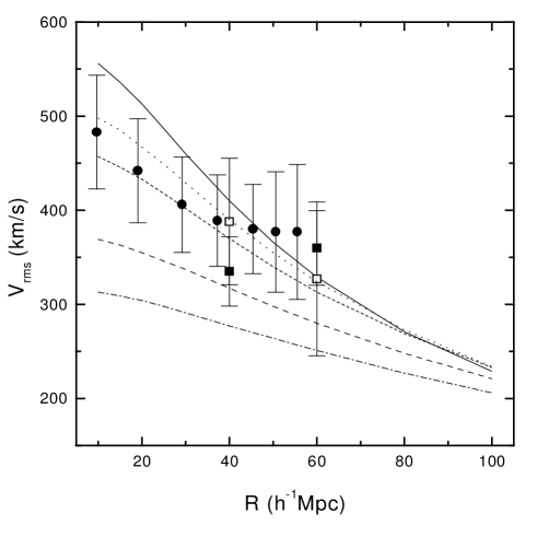
Figure 7: The bulk motion $V_{rms}(R)$ is shown for MLM models with $h=0.5$, $\beta_{H}=2,\beta_{\nu}=4$, $\Omega_{H}/\Omega_{M}=0.2$ and different values of the $\Omega_{\Lambda}$ parameter: $\Omega_{\Lambda}=0$ (solid line), $\Omega_{\Lambda}=0.31$ (dotted line), $\Omega_{\Lambda}=0.45$ (short dashed line), $\Omega_{\Lambda}=0.65$ (long dashed line), $\Omega_{\Lambda}=0.74$ (dot-short dashed line). The solid circles correspond to Dekel(1994), open squares to Bertschinger et al.(1990), solid squares to Courteau et al. (1993)

4.3 Cluster-cluster correlations

The space distribution of rich clusters is a powerful tool for probing the power spectrum at intermediate and large scales. The first attempts to measure the two-point spatial autocorrelation function $\xi_{cc}(r)$ ([Bahcall & Soneira 1983], [Klypin & Kopylov 1983]) have shown that they are more clustered than galaxies and $\xi_{cc}(r)\approx(r_{0}/r)^{\gamma}$ with $\gamma=1.6-2.0$ and $r_{0}=16-25\;h^{-1}Mpc$.

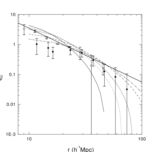
Figure 8: The cluster-cluster correlation functions $\xi_{cc}$ are shown for MLM models with $h=0.5$, $\beta_{H}=2,\beta_{\nu}=4$, $\Omega_{H}/\Omega_{M}=0.1$ and different values of the $\Omega_{\Lambda}$ parameter: $\Omega_{\Lambda}=0$ (solid line), $\Omega_{\Lambda}=0.31$ (dotted line), $\Omega_{\Lambda}=0.45$ (short dashed line), $\Omega_{\Lambda}=0.65$ (long dashed line), $\Omega_{\Lambda}=0.74$ (dot-short dashed line)

The later analysis of other authors (see for example Postman et al. 1992; Olivier et al. 1993; Jing & Valdarnini 1993) has confirmed that $\xi_{cc}$ is well fitted by the same expression with $\gamma=1.8$ and $r_{0}\approx 20\;h^{-1}Mpc$. The important conclusion, which follows from numerous studies of this problem, is the existence of a positive long distance correlation of rich clusters of galaxies out to $50\;h^{-1}Mpc$. For a Gaussian random density fluctuation field the correlation function of peaks at large separations is calculated with the following equation ([Bardeen et al. 1986]):

$$\xi_{cc}(r)={b_{c}^{2}\over 2\pi^{2}}\int_{0}^{\infty}P(k)k^{2}W^{2}(kR_{c}){sin\;kr\over kr}dk,$$

where $W(kR_{c})$ is the window function, which filters out in the density field the structures on scales larger than $R_{c}$, $b_{c}$ is their biasing parameter, which takes into account the statistical correlation of peaks above a given threshold. The biasing parameter is defined by the expression

$$b_{c}=<\tilde{\nu}>/\sigma(R_{c})+1,$$

where the effective threshold level $<\tilde{\nu}>$ is given by

$$<\tilde{\nu}>=\int_{0}^{\infty}d\nu\left(\nu-{\gamma\theta\over 1-\gamma^{2}}\right)t(\nu/\nu_{t})N_{pk}(\nu)/n_{c}$$

with $\gamma$, $\theta$, the threshold function $t(\nu/\nu_{t})$ and the differential number density $N_{pk}(\nu)$ are defined according to equations (4.6a), (6.14), (4.13) and (4.3) of Bardeen et al. (1986). The Gaussian filter radius corresponding to the mass ($M\geq 5\;10^{14}h^{-1}M_{\odot}$) of a rich cluster is $R_{c}=(M/4.35\;10^{12}\Omega_{M}h^{-1})^{1/3}h^{-1}Mpc$. The observed number density of Abell clusters with richness $R\geq 1$, $n^{obs}_{c}=(5.7\pm 0.5)\;10^{-6}h^{3}Mpc^{-3}$ (see [Zamorani et al. 1991]; [Bahcall 1988] for a review), is used for the determination of the peak height $\nu_{t}$

$$n_{c}=\int_{0}^{\infty}d\nu t(\nu/\nu_{t})N_{pk}(\nu)=n^{obs}_{c}.$$

The mean height of peaks for which the rich clusters of galaxies are formed is then

$$<\nu>=\int_{0}^{\infty}d\nu t(\nu/\nu_{t})\nu N_{pk}(\nu)/n_{c}.$$

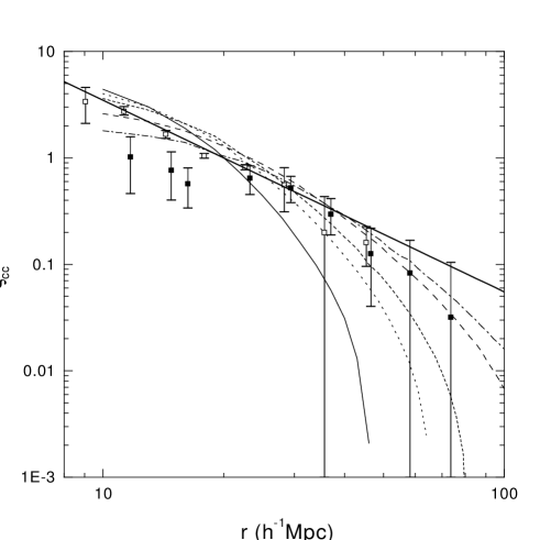
Figure 9: The same as in Fig.8 , but for $\Omega_{H}/\Omega_{M}=0.2$

The cluster-cluster correlation function calculated in this way for the standard CDM scenario strongly conflicts with the one observed , because it becomes negative after $\sim 40\;h^{-1}Mpc$. For the standard MDM models with $\Omega_{H}\leq 0.3$ the situation is better ($\xi_{cc}$ become negative at $\sim 50\;h^{-1}Mpc$) but positive correlations at $>50\;h^{-1}Mpc$ are not explained by them either (see for example [Holtzman & Primack 1993]; [Novosyadlyj 1994]).

The positive correlations at $>50\;h^{-1}Mpc$ would be explained in the cosmological scenario with $\Omega_{M}=1$ and a phenomenological power spectra with enhanced large scale power ([Bardeen, Bond & Efstathiou 1987, Novosyadlyj & Gnatyk 1994, Novosyadlyj 1996]). But such spectra are now ruled out by the data for $\Delta T/T$ at degree angular scales ([Schuster et al. 1993]) because their prediction for the rms $\Delta T/T$ is higher than the 95% c.l. of the experimental upper limit.

An attractive possibility for avoiding this problem is to consider MLM models normalised to the COBE quadrupole. The correlation functions of rich clusters of galaxies calculated as described above agree with observational data and are positive far beyond $50\;h^{-1}Mpc$ (Figs. 8 & 9). As we can see, for MLM models with $0.3\leq\Omega_{M}\leq 0.7$, $\Omega_{H}/\Omega_{M}=0.1\simeq 0.2$ and $h=0.5$ the predicted autocorrelation functions of rich clusters are within the limits of the observed error bars at large distances. A comparison for other $h$ gives the following constraints for $\Omega_{M}h$: $0.13\leq\Omega_{M}h\leq 0.35$.

The biasing parameters of rich clusters of galaxies for all models are in the range $3.3-4.6$ and are in the same range as the values obtained with different methods from observations ([Lynden-Bell 1991, Plionis & Valdarnini 1991, Plionis 1995]). The minimal $\Omega_{M}h$ is constrained also by the moment of turn around of density fluctuation peaks which are associated with rich clusters. Indeed, the requirement that the total cluster mass collapsed before $z=0$ (not only the central region but also the frontier areas ) requires $<\nu>\sigma_{c}\geq 1.06$ ([Bardeen et al. 1986]), which is satisfied for models with $\Omega_{M}h\geq 0.15$ when $\Omega_{H}/\Omega_{M}=0.1$ and $\Omega_{M}h\geq 0.18$ when $\Omega_{H}/\Omega_{M}=0.2$.

4.4 Cluster mass function

The observed abundances of clusters of galaxies is a powerful discriminant for different models of dark matter. We will use the [Press & Schechter 1974] (1974, PS) formula to compute the number density

$$N(>M,z)=\int_{M}^{\infty}n(M^{\prime},z)dM^{\prime},$$

of virialized objects with mass greater than M. According to PS, the comoving number density $n(M,z)$ of halo masses in the interval $M,M+dM$ , is analytically related to the power spectrum by

$$n(M,z)=\sqrt{\frac{2}{\pi}}\frac{\rho_{b}(z)}{M^{2}}\frac{\delta_{c}}{\sigma(M,z)}\left|\frac{dln\sigma}{dlnM}\right|\,e^{-\delta_{c}^{2}/2\sigma^{2}},$$

here $\rho_{b}(z)$ is the background density, $\sigma(M,z)$ is the rms mass density fluctuation and $\delta_{c}$ is the threshold parameter. The rms $\sigma$ value is defined as

$$\sigma^{2}(M,z)=D^{2}(z)\int_{0}^{\infty}\frac{dk}{k}\Delta^{2}(k)W^{2}(k,R),$$

where W is a window function and $D$ is the linear growth factor, $D(0)=1$. The relation between $M$ and $R$ depends on the choice of $W$, for a top-hat function $R=(3M/4\pi\rho_{b})^{1/3}$.

According to linear theory, $\delta_{c}=1.686$, for a top-hat window in an $\Omega_{M}=1$ universe. For the more general case $\Omega_{M}\leq 1$, $\delta_{c}$ can be derived analytically and it has a very weak dependence on $\Omega_{M}$ ([Eke, Cole & Frenk 1996]). On cluster scales, density fluctuations are well described by linear theory and so Eq.(18) is thought to be a good approximation to the true number density. N-body simulations have been used by various authors ([Efstathiou et al. 1988]; [Lacey & Cole 1994]; [Eke, Cole & Frenk 1996] ) for an extensive check of the validity of the PS predictions. In particular Eke et al. (1996) found that Eq.(18) agrees well with N-body results for CDM models in a flat universe.

For a top-hat choice, the best-fit to N-body results is $\delta_{c}=1.7\pm 0.1$, while for a Gaussian window the $\delta_{c}$ threshold is more sensitive to the shape of the power spectra ([Lacey & Cole 1994]). In what follows we will take a top-hat window function $W$ and $\delta_{c}=1.686$. Our results will be compared with those of Ma (1996) , who has made a similar choice. Cluster abundances have been computed for MDM by Ma (1996) ; Bartlett & Silk (1993); Liddle et al. (1996c); Bahcall, Fan & Cen (1997). Clusters of galaxies are rare objects and therefore are very sensitive to the value of $\sigma$ . Our models have two limiting cases: when $\Omega_{\Lambda}\rightarrow 0$ ( MDM models) or when $\Omega_{H}/\Omega_{M}\rightarrow 0$ , which corresponds to $\Lambda$CDM models. For these limiting cases we have compared our integrations with published analytical spectra and found that the greater discrepancies are at high wavenumbers $k\raise-2.0pt\hbox{\hbox to0.0pt{\hbox{$\sim$}\hss}\raise 5.0pt\hbox{$>$}\ }1hMpc^{-1}$ and are $\simeq 10\%$ of the analytical $P(k)$.

Figure 10: The cluster abundance $N(>M)$ is shown at $z=0$ for MDM models with $\Omega_{H}/\Omega_{M}=0.2$, $h=0.5$ and different values of the $\beta_{H}$ and $\beta_{\nu}$ parameters. The values chosen are: $\beta_{H}=2\ \beta_{\nu}=4$ (solid line), $\beta_{H}=6\ \beta_{\nu}=0$ (dotted short line), $\beta_{H}=4\ \beta_{\nu}=2$ (short-dashed line). Data points have been taken from Ma (1996, see text). Black squares correspond to the integration of Ma for the model $\beta_{H}=2\ \beta_{\nu}=4$. The linear spectra used for the calculation of $N(>M)$ are normalized according to the COBE 4-yr data

These differences are mainly due to the absence of baryons in our computations. For the length scale of interest to us, $R\simeq 8-16h^{-1}Mpc$ and the resulting $\sigma$’s will have similar relative errors. Because of the exponential in Eq.(18), the cluster number density is strongly affected by these errors. We have therefore decided to include baryons in our computations of linear spectra. In fact we have obtained the new spectra by taking the computed transfer functions $T(k)$ and interpolating them linearly over a grid of values $q=k/\Omega_{M}h^{2}$.

For the same wavenumber $k$ as in the original computation, the new $T(k)$ is obtained according to the prescription of Sugiyama (1995) : $q\rightarrow q/exp(-\Omega_{b}-\Omega_{b}/\Omega_{M})$. We have taken $\Omega_{b}=0.015/h^{2}$. This procedure works well for CDM transfer functions because, after recombination, baryons are caught by the CDM component and their perturbations grow together. For spectra with a hot component the ratio $T_{H}/T_{CDM}$ to a first approximation does not depend on $\Omega_{M}$ and the prescription can be applied to the total transfer function. For MDM Liddle et al. (1996c) have applied a similar procedure to the transfer functions of Pogosyan & Starobinsky (1995), who do not include baryons in their calculations. They found that the applicability of the procedure requires $\Omega_{b}\raise-2.0pt\hbox{\hbox to0.0pt{\hbox{$\sim$}\hss}\raise 5.0pt\hbox{$<$}\ }0.1$ and $h\raise-2.0pt\hbox{\hbox to0.0pt{\hbox{$\sim$}\hss}\raise 5.0pt\hbox{$>$}\ }0.5$, a range of limits that we never consider.

In order to compare our results with observations we take the number density of clusters at two mass ranges from the work of Ma (1996). These data points correspond to clusters with X-ray temperature greater than 3.7 and 7 keV ( [Henry & Arnaud 1991]). For the first point White et al.( 1993a) estimated the upper limit in mass from the cluster velocity dispersion, while for the lower limit the X-ray temperature of $3.6$ KeV has been converted into a mass of $M=4.2\ 10^{14}M_{\odot}$ assuming an isothermal model. The second point is taken from Liddle et al. (1996d) who have used the N-body hydro simulations of White et al. (1993b) and found $M=(1.23\pm 0.3)10^{15}h^{-1}M_{\odot}$ for the virial mass of a cluster with $X$-ray temperature $kT=7$ keV in a critical universe.

Figure 11: The same as in Fig. 10 but for MDM models with $h=0.5$, $\beta_{H}=2,\beta_{\nu}=4$, and $\Omega_{H}/\Omega_{M}=0.1$ (solid line), $\Omega_{H}/\Omega_{M}=0.2$ (dotted line), $\Omega_{H}/\Omega_{M}=0.3$ (short dashed line)

In Fig. 10 we plot the present mass functions of clusters for SMDM models with $\Omega_{H}=0.2,h=0.5,\Omega_{b}=0.06$. The figure shows the dependence of $N(>M)$ on the number of species of massless and massive collisionless particles. We assume that the total number of species of both particles is equal to $3$. We can see a weak dependence on these parameters. The mass function in SMDM models with one species of massive neutrinos is above that for models with three massive neutrinos. Keeping $\Omega_{H}$ fixed, and decreasing the neutrino mass, then $N(>M)$ decreases too. It can be seen that the model with $\beta_{H}=4$, advocated by Primack et al. (1995), fares much better.

Fig. 11 shows the mass function $N(>M)$ for SMDM models with different values of $\Omega_{H}=0.1,0.2,0.3$ and fixed values of $h=0.5,\beta_{H}=2,\beta_{\nu}=4$. The black squares correspond to the $\Omega_{H}=0.2$ case treated by Ma (1996, figure 8 top right). With an increase of $\Omega_{H}$, the mass function decreases. We can observe also small differences in the shape of the functions.

As we can see, for the considered range of parameters SMDM models do not fit cluster abundances, if we adopt the COBE normalization and spectral index $n=1$ with no gravitational waves. The $\Omega_{H}=0.3$ case is marginally consistent, and it was the one considered by Bartlett & Silk (1993). An improvement in the fit can be obtained with the introduction of a small tilt in the initial spectrum ( $n\simeq 0.9$ ) and/or a tensor contribution to COBE anisotropies. This point has been discussed in detail by Ma (1996) and we do not consider it here.

For MLM models the data points in Fig. 11 should be calculated according to the model, because the conversion from temperatures to masses depends on $\Omega_{M}$. For this reason we next consider the cumulative cluster temperature function predicted for different MLM models, and compare it with observations.

4.5 Cluster temperature function

Identification of clusters of galaxies in the optical band is subject to the problems of foreground/background contamination. Projection effects can also undermine mass determination through virial analysis ([Frenk et al. 1990]; [Dekel et al. 1989]). On the other hand clusters are also strong X-ray sources ([McKee et al. 1980]), their emission does not suffer from these problems and clusters can be reliably identified.

The X-ray emission of galaxy clusters has two physical observable- related quantities: the luminosity and the temperature. During cluster collapse, the gas is shock heated to the virial temperature, then it approaches an isothermal distribution in virial equilibrium. For the gas temperature $T_{g}$ one should have $T_{g}\propto\alpha M^{2/3}$. This relation has been confirmed by numerical simulations ( [Evrard, Metzler & Navarro 1996]; [Navarro, Frenk & White 1995]) with a very small dispersion for the coefficient $\alpha$ and different DM models.

Then the $T-M$ relation allows us to connect the PS equation (18) to the cluster X-ray temperature function (XTF). We take the Eke, Cole & Frenk (1996, hereafter ECF) relation for an isothermal gas:

$$kT_{gas} = {7.75\over\beta}\left({6.8\over{5X+3}}\right){\left({M\over{10^{15}h^{-1}M_{\cdot}}}\right)}^{2\over 3}(1+z)$$ (20)

$$\times{\left({\Omega_{M}\over\Omega_{M}(z)}\right)}^{1\over 3}{\left({\Delta_{c}\over 178}\right)}^{1\over 3}keV,$$

here $\beta$ is the ratio of the galaxy kinetic energy to the gas thermal energy, $X$ is the hydrogen mass fraction, $\Delta_{c}$ is the ratio of the mean halo density within a virial radius to the critical density at the corresponding redshift. We assume $X=0.76$, $\beta=1$ and $\Delta_{c}=178$ (ECF). For $\Omega_{M}<1$, $\Delta_{c}$ can be derived analytically and is well approximated by $\Delta_{c}=178\Omega_{M}^{0.45}$.

Figure 12: We show the temperature function of clusters $N(>kT)$ for MLM models with $h=0.5$, $\beta_{H}=2,\beta_{\nu}=4$, $\Omega_{H}/\Omega_{M}=0.2$ and different values of the $\Omega_{\Lambda}$ parameter: $\Omega_{\Lambda}=0.$ (solid line), $\Omega_{\Lambda}=0.31$ (dotted line), $\Omega_{\Lambda}=0.45$ (short dashed line), $\Omega_{\Lambda}=0.65$ (long dashed line), $\Omega_{\Lambda}=0.74$ (dot-short dashed line). The histogram is obtained from the X-ray data set of Henry and Arnaud (1991). Open squares are three selected temperatures for which error bars have been estimated with a bootstrap procedure. Black circles refer to the mass function of Bahcall and Cen (1993). The horizontal bar is from White et al.(1993a)

For a specified model Eqs.(18-20) allow us to compute the cluster XTF $N(>kT)$. Then this function can be compared with present data and can be used to constrain different DM models ([Bartlett & Silk 1993]; ECF; [Viana & Liddle 1996]). Current observations from Einstein and EXOSAT satellites have been used to determine the local cluster XTF ([Henry & Arnaud 1991]; [Edge et al. 1990]). Our study of the cluster XTF will make use of the Henry & Arnaud (1991) data. In particular we will closely follow the analysis of ECF, this will make it easy to compare of our MLM predictions with previous result for $\Lambda$CDM models (ECF).

The estimated cumulative cluster XTF is computed according to

$$N(>kT)=\sum_{T_{i}>T}1/V_{max,i}\ ,$$

here $V_{max,i}$ is the maximum volume at which the $i-th$ cluster can be detected for a specified flux limit ($F_{X}=3\,10^{-11}ergsec^{-1}cm^{-2}$) in the $2-10$ Kev range.

The cumulative XTF obtained in this way is shown as the solid line histogram in Fig. 12. Error bars have been found with a bootstrap procedure, applied to the original sample of 25 clusters, at three different temperature bins $T_{j}$. The resulting $1\sigma$ amplitudes $\delta_{j}$ are plotted as open squares in Fig. 12, at the three corresponding temperatures. The $\delta^{2}_{j}$ are defined as $\delta^{2}_{j}=<(\log_{10}N^{boot}(>kT_{j})-\overline{\log_{10}N^{boot}(>kT_{j})})^{2}>$, the average being over the bootstrap ensemble.

The estimated $N(>kT)$ agrees with the one obtained by ECF (see their Fig. 3), the procedure being the same, and is consistent with the differential one of Henry & Arnaud (1991), although ECF pointed out some errors in the original estimate that almost cancel each other.

The horizontal bar on the left upper part is the first data point of the previous $N(>M)$ figures. The point was obtained from White et al.(1993a) precisely from the temperature function of Henry & Arnaud (1991) and it proves the consistency of our procedure. The small offset along the $kT$ axis can be attributed to the use of the differential or cumulative temperature functions (ECF).

A different test is to compare our $N(>kT)$ with the cluster mass function of Bahcall & Cen (1993). Their best fit $N(>M)$ is plotted as black circles for three different temperatures. In order to convert masses into temperatures we have used Eq.(5) of Bahcall & Cen (1993). Error bars represent the $1\sigma$ dispersion of their Eq.(5). As can be seen, there is a substantial agreement between the two estimates.

In comparing the predictions of our models with the observed XTF one must be aware of possible uncertainties in the mass-temperature relation. Because of the steep decline of the XTF with temperature, even a small dispersion can have drastic effects. In Eq.(20) the parameter $\beta$ represents the ratio between the virial and gas temperatures (we have assumed an isotropic isothermal profile). The $\beta$ parameter can be calculated either from the data or through numerical simulations.

Current available data are consistent with $\beta\simeq 1$ ([Edge & Stewart 1991]; [Squires at al. 1996]). The hydrodynamical simulations of Navarro, Frenk & White (1995) give a result of $\beta\simeq 1$ and have been used by ECF , who assume $\beta=1\pm 0.1$. This scatter around unity for $\beta$ ( $\simeq 10\%$) has been confirmed in more recent work by Eke, Navarro & Frenk (1997, see also [Evrard, Metzler & Navarro 1996]), who have performed a set of N-body hydrodynamical simulations to investigate the X-ray evolution for a set of clusters in a low-density flat CDM cosmology.

Thus we have reliably assumed $\beta=1$ in order to convert masses into temperatures. The theoretical XTF has then been computed from Eq.(18), for MLM models with different $\Omega_{\Lambda}$ and a fixed ratio $\Omega_{H}/\Omega_{M}=0.2$. We normalize the final spectra according to the COBE data (see sect.2.2 ). The results are shown in Fig. 12.

Figure 13: The same as in Fig.12, but for $\Omega_{H}/\Omega_{M}=0.1$

The inclusion of a $\Lambda$ term clearly alleviates the problem for MDM and brings the models in good agreement with the data. The solid line is the limiting case $\Omega_{\Lambda}=0$, which corresponds to the standard MDM. In order to fit the present cluster abundance, this model would require a value $\beta\simeq 2$, clearly inconsistent with present estimates.

Figure 14: a $\sigma_{8}$ is shown as a function of $\Omega_{M}$ for MLM models with $h=0.5,\beta_{H}=2,\beta_{\nu}=4$, $\Omega_{H}/\Omega_{M}=0.2$. The continuous line is the best-fit to the estimated cluster abundance, the dashed line is from the COBE 4-yr data. The thin lines show the statistical uncertainties, quoted in the text. b The same as in panel a, but for $\Omega_{H}/\Omega_{M}=0.1$

From Fig. 12 the best range of $\Omega_{\Lambda}$ for fitting the data is $\Omega_{\Lambda}\simeq 0.3-0.5$. Fig. 13 shows the same plot of Fig. 12 , but for $\Omega_{H}/\Omega_{M}=0.1$. In this case the best range for $\Omega_{\Lambda}$ is $\simeq 0.4-0.6$. In order to constrain a particular model we can now compute the $\chi^{2}$ quantity

$$\chi^{2}=\sum_{j=1}^{3}\sum_{k=1}^{3}y_{j}C_{jk}^{-1}y_{k},$$

where $j$ is the bin index, $y_{j}=(\log_{10}(N_{j})-\log_{10}(N_{j}^{th}))$, $N_{j}=N(>kT_{j})$ and $N_{j}^{th}$ is for a particular model from Eq.(18). The covariance matrix $C_{jk}=<\delta_{j}\delta_{k}>$ takes into account the correlations between different temperature bins. According to ECF these correlations are not negligible, but the models which minimize $\chi^{2}$ do not depend strongly on their inclusion in Eq.(22). Thus ECF take for $C_{kl}$ its diagonal form. However the models that we consider have different spectra and we have chosen to keep the whole matrix for the minimization of Eq.(22).

From Eqs.(18-19) $\chi^{2}$ is a function of the power spectrum constant $A$ or, equivalently, of the rms mass fluctuation $\sigma_{8}\equiv\sigma(R=8h^{-1})$. From the minimization of Eq.(22) the formal error on $\sigma_{8}$ is 5 %, but uncertainties on the other parameters will affect $\sigma_{8}$ too. From N-body integrations ECF assume a scatter of 4 % for $\delta_{c}$. This is not surprising because for the length scale of interest to us we can neglect tidal forces and assume that the collapse is spherically symmetric. Other sources of errors are the scatter in $\beta$ ( $\sim$$<$ 10 % ) , the sample completeness ( 90 % at $F_{X}=3\ 10^{-11}ergsec^{-1}cm^{-2}$, [Lahav et al. 1989] ) and errors in the measurement of temperatures. For the latter error, ECF analysis gives an upper limit of $\sim$$<$ 1 %. Summing all these errors in quadrature the final dispersion for $\sigma_{8}$ is about 10 %, twice the statistical error.

For a given model we can now estimate, from Eq.(22), the $\sigma_{8}$ which is consistent with the estimated cluster abundance, and compare it with the $\sigma_{8}$ obtained from COBE data. These two values for $\sigma_{8}$ will in general not coincide, however there will be a set of values of cosmological parameters for which they will be in the same range. The estimated uncertainties allow us to judge the reliability of the overlap. For the COBE normalization we have assumed a 7 % statistical error ([Bunn & White 1997]).

We show in Fig. 14a the $\sigma_{8}$ ( continuous line ) which is obtained from the minimization of the $\chi^{2}$ quantity. The dashed line is from COBE. The two sigmas are plotted as function of the cosmological parameter $\Omega_{M}$. The set of models is for $h=0.5$ and $\Omega_{H}/\Omega_{M}=0.2$. Thin lines represent the assumed uncertainties.

From Fig. 14a the best range of $\Omega_{M}$ which fits the data is $0.55\raise-2.0pt\hbox{\hbox to0.0pt{\hbox{$\sim$}\hss}\raise 5.0pt\hbox{$<$}\ }\Omega_{M}\raise-2.0pt\hbox{\hbox to0.0pt{\hbox{$\sim$}\hss}\raise 5.0pt\hbox{$<$}\ }0.75$. The standard MDM model ($\Omega_{M}=1$) is rejected at the $2\sigma$ level. Fig. 14b shows the same plot as in panel (a), but for $\Omega_{H}/\Omega_{M}=0.1$. In this case the best range for $\Omega_{M}$ is $0.45\raise-2.0pt\hbox{\hbox to0.0pt{\hbox{$\sim$}\hss}\raise 5.0pt\hbox{$<$}\ }\Omega_{M}\raise-2.0pt\hbox{\hbox to0.0pt{\hbox{$\sim$}\hss}\raise 5.0pt\hbox{$<$}\ }0.65$. In Fig.15 we consider the same set of models but for $h=0.7$. We obtain $0.3\raise-2.0pt\hbox{\hbox to0.0pt{\hbox{$\sim$}\hss}\raise 5.0pt\hbox{$<$}\ }\Omega_{M}\raise-2.0pt\hbox{\hbox to0.0pt{\hbox{$\sim$}\hss}\raise 5.0pt\hbox{$<$}\ }0.5$ for $\Omega_{H}/\Omega_{M}=0.2$ and $0.3\raise-2.0pt\hbox{\hbox to0.0pt{\hbox{$\sim$}\hss}\raise 5.0pt\hbox{$<$}\ }\Omega_{M}\raise-2.0pt\hbox{\hbox to0.0pt{\hbox{$\sim$}\hss}\raise 5.0pt\hbox{$<$}\ }0.4$ when $\Omega_{H}/\Omega_{M}=0.1$.

Figure 15: a $\sigma_{8}$ is plotted versus $\Omega_{M}$ for MLM models with $h=0.7,\beta_{H}=2,\beta_{\nu}=4$, $\Omega_{H}/\Omega_{M}=0.2$. The meaning of the lines is the same as in Fig.14. b The same as in panel a, but for $\Omega_{H}/\Omega_{M}=0.1$

According to the value of $h$ we can then summarize the following constraints for MLM models with one species of massive neutrinos and $\Omega_{H}/\Omega_{M}\leq 0.2$: $0.5\raise-2.0pt\hbox{\hbox to0.0pt{\hbox{$\sim$}\hss}\raise 5.0pt\hbox{$<$}\ }\Omega_{M}\raise-2.0pt\hbox{\hbox to0.0pt{\hbox{$\sim$}\hss}\raise 5.0pt\hbox{$<$}\ }0.8$ ($h=0.5$) or $0.3\raise-2.0pt\hbox{\hbox to0.0pt{\hbox{$\sim$}\hss}\raise 5.0pt\hbox{$<$}\ }\Omega_{M}\raise-2.0pt\hbox{\hbox to0.0pt{\hbox{$\sim$}\hss}\raise 5.0pt\hbox{$<$}\ }0.5$ ($h=0.7$). The corresponding allowed values of $\sigma_{8}$ are : $\sigma_{8}\simeq 0.65\pm 0.1$ ($h=0.5$) or $\sigma_{8}\simeq 0.8\pm 0.1$ ($h=0.7$). A comparison of these constraints with the clustering data of sect.4.1 must take into account the biasing factor. A rescaling of $\Delta^{2}(k)$ according to $b_{gal}=1/\sigma_{8}$ shows that consistency with cluster abundance is marginal for models with $\Omega_{H}/\Omega_{M}=0.2$. For $h=0.5$ and $\Omega_{H}/\Omega_{M}=0.1$ we obtain $0.55\raise-2.0pt\hbox{\hbox to0.0pt{\hbox{$\sim$}\hss}\raise 5.0pt\hbox{$<$}\ }\Omega_{M}\raise-2.0pt\hbox{\hbox to0.0pt{\hbox{$\sim$}\hss}\raise 5.0pt\hbox{$<$}\ }0.65$ , while for $h=0.7$ the limits on $\Omega_{M}$ are $0.35\raise-2.0pt\hbox{\hbox to0.0pt{\hbox{$\sim$}\hss}\raise 5.0pt\hbox{$<$}\ }\Omega_{M}\raise-2.0pt\hbox{\hbox to0.0pt{\hbox{$\sim$}\hss}\raise 5.0pt\hbox{$<$}\ }0.4$.

The constraints on $\Omega_{M}$ that we obtain follow from comparing our results with the present cluster XTF. We have not considered possible constraints that might be given by considering cluster evolution. The evolution of cluster number density with redshift is a powerful tool for discriminating among different cosmologies. This follows directly from the different growth of density fluctuations in different cosmologies. The fluctuations in models with $\Omega_{M}<1$ grow very slowly and structures will experience little evolution at recent times. On the contrary, for $\Omega_{M}=1$, the higher growth rate of density fluctuations implies for galaxy clusters a much stronger evolution at late redshifts.

Bahcall, Fan & Cen (1997) compared the results for cluster abundance, using large-scale N-body simulations, with recent data at $z\simeq 0.5-1$. They found that MDM models are ruled out at the $2\sigma$ level, while a $\Lambda$CDM model with $\Omega_{M}=0.34\pm 0.13$ $h=0.65$ can consistently fit the data. These simulations show that the cluster evolution rate is strongly model dependent. We accordingly do not attempt here to perform a linear analysis, applying Press-Schechter theory, to compute the redshift evolution of the cluster number density for MLM models.

We suggest then that large scale numerical simulations can be used to compare the cluster evolution for MLM models with recent data. These tests are likely to strengthen or falsify the models, given the already narrow window of allowed values for the cosmological parameters arising from the linear tests applied here.

4.6 Damped Lyman-$\alpha$ systems

An important test for dark matter models with a massive neutrino component is given from the observations of objects at high redshifts. Due to free-streaming effects the dark matter power spectrum will be severely damped on small scales, thus making formation of early objects more difficult than in a model without the hot component. The most important class of such objects are damped Lyman-$\alpha$ absorption systems.

These objects have a high column density of neutral hydrogen ($N_{HI}\raise-2.0pt\hbox{\hbox to0.0pt{\hbox{$\sim$}\hss}\raise 5.0pt\hbox{$>$}\ }10^{20}cm^{-2}$) and are detected by means of absorption lines in quasar spectra (Wolfe 1993). Observations at high redshift have lead to estimates of the abundance of neutral hydrogen in damped Lyman-$\alpha$ systems (Lanzetta, Wolfe & Turnshek 1995; Storrie-Lombardi et al. 1996). The latter authors have analyzed spectra at $z=3$ and $z=4$ , we will make use of the $z=4$ data, which gives the strongest constraint on the primordial spectrum. According to Storrie-Lombardi et al. (1996), the cosmological mass density of neutral hydrogen gas $\Omega_{g}$ is given by

$$\Omega_{g}(z=4)=(0.0011\pm 0.0002)h^{-1}\sqrt{\frac{\Omega_{M}}{\Omega_{M}(z=4)}},$$

with the original data being given in units of the critical density, the square root taking into account different cosmologies.

The standard view is that damped Lyman-$\alpha$ systems are a population of protogalactic disks ([Wolfe 1993]), with a minimum mass of $M\geq 10^{10}h^{-1}M_{\odot}$ ([Haehnelt 1995]). The fractional density of collapsed objects of minimum mass $M_{DLAS}$ is then

$$\Omega_{DLAS}(z=4) = \frac{\Omega_{g}(z=4)}{f_{gas}\Omega_{b}}=(0.069\pm 0.021)\frac{h}{f_{gas}}$$ (24)

$$\times\sqrt{\frac{\Omega_{M}}{\Omega_{M}(z=4)}}$$

where $f_{gas}$ is the fraction of neutral hydrogen and $\Omega_{b}=0.016h^{-2}$ ([Copi, Schramm & Turner 1995]). In Eq. (24) the error in $\Omega_{b}$ has been added in quadrature (Liddle et al. 1996c). A conservative assumption is $f_{gas}=1$, but recent hydrodynamical simulations ([Ma et al. 1997]) have claimed $f_{gas}\leq 0.1$. We will consider constraints on our models arising from both of the limits on $f_{gas}$.

Figure 16: $\sigma(M,z=4)$ is shown as a function of $\Omega_{M}$ for $h=0.5$. The continuous line represents the 95 confidence level for the the lower limit obtained from observational data using Press-Schechter theory. The bottom line is for $f_{gas}=1$ and the top line refers to $f_{gas}=0.1$. The $\sigma(M,z=4)$ for MLM models are plotted as dashed lines for different values of the ratio $\Omega_{H}/\Omega_{M}$. The long(short)-dashed line is for $\Omega_{H}/\Omega_{M}=0.2(0.1)$

The theoretical counterpart of Eq.(24) can be found using the Press-Schechter (1974) theory and is given by

$$\Omega_{DLAS}(>M,z)={\rm erfc}\left[\frac{\delta_{c}}{\sqrt{2}\sigma(M,z)}\right],$$

where erfc is the complementary error function and $\sigma(M,z)$ is defined according to Eq.(19) using a top-hat window function. Particular care must be taken when inserting the minimum mass into Eq.(19) because for damped Lyman-$\alpha$ systems $M=M_{DLAS}$ is well below the neutrino clustering scale at $z=4$. We correct $M_{DLAS}$ according to $M_{DLAS}\rightarrow 10^{10}h^{-1}(1-\Omega_{H}/\Omega_{M})^{-1}M_{\odot}$ (Liddle at al. 1996c). The collapsed state of damped Lyman-$\alpha$ systems is uncertain and a conservative assumption is that these systems have collapsed along two axes. We accordingly take for the threshold parameter the value $\delta_{c}=1.5$ (Monaco 1995).

We conservatively assume the theoretical predictions (25) to be bounded from below by Eq.(24), for $\Omega_{DLAS}$ we take the $2\sigma$ lower limit. The rms mass fluctuation $\sigma(M,z=4)$ can now be constrained from below using Eqs.(24-25). We show these limits as a function of $\Omega_{M}$ in Figs. 16 & 17, for $h=0.5$ and $h=0.7$, respectively. In these figures the bottom solid line is for $f_{gas}=1$, while the top solid line refers to $f_{gas}=0.1$. This value gives a much more severe constraint on $\sigma(M,z=4)$ than for $f_{gas}=1$. The theoretical values of $\sigma(M,z=4)$ are shown for $\Omega_{H}/\Omega_{M}=0.1$ ( short dashed line ) and $\Omega_{H}/\Omega_{M}=0.2$ ( long dashed line ). At a given $\Omega_{M}$ the value of $\sigma(M,z=4)$ decreases as the ratio $\Omega_{H}/\Omega_{M}$ increases. This behavior of $\sigma(M,z=4)$ follows because an increase of $\Omega_{H}$ implies, for a given normalization and redshift, a reduction in the available power at small scales. The effect becomes more pronounced for $\Omega_{M}\rightarrow 1$

From Fig. 16 one can infer that for $h=0.5$ MLM models with $\Omega_{H}/\Omega_{M}=0.1$ are not strongly constrained by the available data for damped Lyman-$\alpha$ systems. For $h=0.5$ and $\Omega_{H}/\Omega_{M}=0.2(0.1)$ we obtain the following lower limits : $0.8(0.4)\raise-2.0pt\hbox{\hbox to0.0pt{\hbox{$\sim$}\hss}\raise 5.0pt\hbox{$<$}\ }\Omega_{M}$. For $\Omega_{H}/\Omega_{M}=0.2$ this lower limit on $\Omega_{M}$ do not overlap with the upper limit given by cluster abundances and the model is inconsistent. For $h=0.7$ we obtain from Fig. 17 $0.4(0.2)\raise-2.0pt\hbox{\hbox to0.0pt{\hbox{$\sim$}\hss}\raise 5.0pt\hbox{$<$}\ }\Omega_{M}$ if $\Omega_{H}/\Omega_{M}=0.2(0.1)$. This lower limit is consistent with the upper limits from cluster abundances and other constraints for the same set of models.

These constraints on $\Omega_{M}$ have been obtained for a minimum mass of $M=10^{10}h^{-1}M_{\odot}$, the role of possible uncertainties on the limits for $\Omega_{M}$ can be considered by decreasing this lower limit by an order of magnitude. For $M=10^{9}h^{-1}M_{\odot}$ we obtain new constraints on $\Omega_{M}$ which do not differ in a relevant way from those shown in Figs. 16 & 17.

Figure 17: The same as in Fig.16, but for $h=0.7$

We have considered $f_{gas}=1$ but if we take $f_{gas}=0.1$ then none of the MLM models for $h=0.5$ survives the constraints from damped Lyman-$\alpha$ systems. The model with $\Omega_{H}/\Omega_{M}=0.2$ is excluded and $\Omega_{H}/\Omega_{M}=0.1$ requires $\Omega_{M}\raise-2.0pt\hbox{\hbox to0.0pt{\hbox{$\sim$}\hss}\raise 5.0pt\hbox{$>$}\ }0.8$, a minimum value excluded at the $1\sigma$ level by cluster abundances. Also MLM models with $h=0.7$ are severely constrained if $f_{gas}=0.1$. In this case we have $\Omega_{M}\raise-2.0pt\hbox{\hbox to0.0pt{\hbox{$\sim$}\hss}\raise 5.0pt\hbox{$>$}\ }0.8(0.4)$ for $\Omega_{H}/\Omega_{M}=0.2(0.1)$. Thus the model with $\Omega_{H}/\Omega_{M}=0.2$ is totally inconsistent with cluster abundances but $\Omega_{H}/\Omega_{M}=0.1$ is still within the $1\sigma$ range. We conservatively take the lower limit on $\Omega_{M}$ arising from $f_{gas}=1$. Numerical hydrodynamical simulations have tested only MDM models ([Ma et al. 1997]), hydro simulations with MLM spectra are clearly required in order to obtain a tight limit on $f_{gas}$.

5 Conclusions

We have discussed linear clustering evolution for a set of spatially flat MDM models with a cosmological constant. We have not considered the role of gravitational waves or of a possible tilt in the primordial spectrum. In order to restrict the range of allowed values for the cosmological parameters, we have applied linear perturbation theory to compare the predictions of our MLM models with a set of linear data. The models considered had one species of massive neutrinos and a scale-invariant spectrum.

Linear calculations for the dimensionless power spectra $\Delta^{2}(k)$ have been compared with the reconstructed real-space power spectrum of Peacock & Dodds (1994), Peacock (1997). Because we have considered linear spectra evolution a comparison of clustering is meaningful only at low $k$ ($\raise-2.0pt\hbox{\hbox to0.0pt{\hbox{$\sim$}\hss}\raise 5.0pt\hbox{$<$}\ }0.2hMpc^{-1})$ A substantial agreement is obtained for those unbiased models with $\Omega_{H}/\Omega_{M}\raise-2.0pt\hbox{\hbox to0.0pt{\hbox{$\sim$}\hss}\raise 5.0pt\hbox{$<$}\ }0.2$, and $\Omega_{M}\raise-2.0pt\hbox{\hbox to0.0pt{\hbox{$\sim$}\hss}\raise 5.0pt\hbox{$>$}\ }0.6$ ($h=0.5$) or $0.3\raise-2.0pt\hbox{\hbox to0.0pt{\hbox{$\sim$}\hss}\raise 5.0pt\hbox{$<$}\ }\Omega_{M}\raise-2.0pt\hbox{\hbox to0.0pt{\hbox{$\sim$}\hss}\raise 5.0pt\hbox{$<$}\ }0.5$ ($h=0.7$).

The computed linear power spectra have been filtered with a Gaussian window of radius $R_{f}=12h^{-1}Mpc$ to calculate the peculiar velocity field. A comparison of the rms bulk motion with POTENT data does not lead to strong constraints : $\Omega_{\Lambda}\raise-2.0pt\hbox{\hbox to0.0pt{\hbox{$\sim$}\hss}\raise 5.0pt\hbox{$<$}\ }0.7$ and $\Omega_{H}/\Omega_{M}\raise-2.0pt\hbox{\hbox to0.0pt{\hbox{$\sim$}\hss}\raise 5.0pt\hbox{$<$}\ }0.2$. The cluster-cluster correlation functions calculated for MLM spectra in the framework of Gaussian random density fluctuation field explain the observed positive correlations at $>50\;h^{-1}Mpc$ and are within the limits of the error bars for that observed at large distances when $0.13\leq\Omega_{M}h\leq 0.35$.

Of the considered tests the most important turns out to be that based on cluster abundances, for which the present X-ray cluster temperature function can put strong limits on the initial spectrum amplitude, or conversely on $\sigma_{8}$. Because of the strong dependence of $N_{cl}(>kT)$ on temperature, the conversion of X-ray temperatures into masses is critical . From the discussion of Section 4.5 this conversion can be obtained with a dispersion of less than 10 %. We have then used the Press & Schechter (1974) formalism to compute the cluster number density for different MLM models. Consistency with present data can be achieved for COBE normalized models only for the following range of values (at $1\sigma$ level): $\Omega_{H}/\Omega_{M}\leq 0.2$, $h=0.5(0.7)$ and $0.45(0.3)\leq\Omega_{M}\leq 0.75(0.5)$. In correspondence with these limits, the allowed values of $\sigma_{8}$ are : $\sigma_{8}\simeq 0.65\pm 0.1$ ($h=0.5$) or $\sigma_{8}\simeq 0.8\pm 0.1$ ($h=0.7$). These limits suggest that MLM models require a moderate amount of bias to be consistent with clustering data. For these range of values consistency with clustering data yields $0.55(0.35)\leq\Omega_{M}\leq 0.65(0.4)$ for $h=0.5(0.7)$ and $\Omega_{H}/\Omega_{M}=0.1$. Models with $\Omega_{H}/\Omega_{M}=0.2$ are almost inconsistent.

One can also compare these constraints with those given by considering cluster evolution. The evolution of galaxy clusters has recently been used also for determining the cosmological parameters $\sigma_{8}$ and $\Omega_{M}$. Fan, Bahcall & Cen (1997) found $\sigma_{8}=0.83\pm 0.15$. This range of values is consistent with the $\sigma_{8}$ required for MLM with $h=0.7$ (Fig. 15), and marginally consistent if $h=0.5$. At the $2\sigma$ level none of the MLM models considered here is ruled out. Finally Henry (1997) has used recent data for the evolution of the cluster X-ray temperature function to determine $\Omega_{M}$ and $\sigma_{8}$. For a flat cosmology he obtains $\Omega_{M}=0.55\pm 0.17$ and $\sigma_{8}=0.66^{+0.34}_{-0.17}$, in close agreement with our findings for MLM models.

The observed abundance of damped Lyman-$\alpha$ systems has been used to obtain lower limits on the rms mass fluctuation $\sigma(M)$ at $z=4$ using Press-Schechter theory. These limits yield the following constraints on $\Omega_{M}$ for MLM models with $\Omega_{H}/\Omega_{M}\leq 0.2$ : $0.8-0.4(0.3)\raise-2.0pt\hbox{\hbox to0.0pt{\hbox{$\sim$}\hss}\raise 5.0pt\hbox{$<$}\ }\Omega_{M}$ for $h=0.5$ ($h=0.7)$. These values have been obtained assuming the fraction of neutral hydrogen to be unity. If this fraction is close to $10\%$, as suggested by numerical hydro simulations, then the constraints for MLM models become much more severe. In this case consistency with both damped Lyman-$\alpha$ and cluster abundances can be achieved only for $h=0.7$ , $\Omega_{M}\simeq 0.4$ and $\Omega_{H}/\Omega_{M}=0.1$.

In order to further restrict our models we can also consider present observational constraints on cosmological parameters. The cosmological constant is constrained to be $\Omega_{\Lambda}\leq 0.66$ at the 95 % confidence limit by QSO lensing (Kochanek 1996). A tighter restriction comes from the recent work of Perlmutter et al. (1997) on SN Ia , who give $\Omega_{\Lambda}<0.51$ still at 95 % c.l. .

Recent Hipparcos data ( Feast & Catchpole 1997, Reid 1997) have brought down the Cepheid scale distance, thus reducing the estimated Globular Cluster age to $t_{0}>12Gyr$ and $h$ to a mid term $h=.65$. These values still require a cosmological constant, but not as high as in $\Lambda$CDM models. A value of $\Omega_{\Lambda}>0.4$ is needed to satisfy the new age constraint.

An upper limit on $\Omega_{M}$ can be obtained from the estimated baryonic content of galaxy clusters. If clusters are massive enough to represent a fair sample of the total matter content in the universe, as numerical simulations confirm ([Evrard, Metzler & Navarro 1996]), then the baryon fraction $f_{b}=(0.06\pm 0.003)h^{-3/2}$ (Evrard 1997) should be close to its universal value.

Thus the standard Big Bang Nucleosynthesis value $\Omega_{b}=(0.008-0.024)h^{-2}$ ([Copi, Schramm & Turner 1995]) can be used to infer $\Omega_{M}=\Omega_{b}/f_{b}=(0.25\pm 0.15)h^{-1/2}$. For $h=0.65$ one obtains $\Omega_{M}<0.5$. For a flat model this limit already overlaps the lower limit from SN Ia. This is the main argument for a cosmological constant, possible counter arguments like a magnetic field pressure or density inhomogeneities, which can lead to underestimate the total cluster mass, are unlikely to push the limit up to $\Omega_{M}=1$ ( Evrard 1997 and references cited therein ).

The region of parameter space which is allowed by these observational constraints for a flat model is then: $0.5\leq h\leq 0.7$, $0.3\leq\Omega_{M}\leq 0.6$. These are also the limits that for MLM models the cosmological parameters must independently satisfy in order to achieve consistency with the set of linear clustering data previously analysed.

We think that this is a notable feature of MLM models and one of the most important results of this paper. We then summarize our conclusions by saying that MLM models appear to be a promising class of cosmological dark matter models. Our linear analysis shows that consistency for the cosmological parameters is achieved over a wide range of observational data.

Acknowledgements

T. Kahniashvili is grateful to ICTP and SISSA for financial support and B. Novosyadlyj also acknowledges financial support by SISSA. T.K. and B.N. are grateful to SISSA for hospitality and the stimulating academic atmosphere which allowed this work to progress. RV thanks also S. Bonometto for helpful discussions.

References

- [Achilli, Occhionero & Scaramella 1985] Achilli, S., Occhionero, F., & Scaramella, R. 1985, ApJ 299, 577
- [Bahcall & Soneira 1983 ] Bahcall, N.A., & Soneira, R.M. 1983, ApJ 270, 20
- [Bahcall 1988] Bahcall, N. 1988, ARA&A 26, 631
- [Bahcall 1996] Bahcall, N. 1996, astro-ph/9612046
- [Bahcall & Cen 1993] Bahcall, N.A., & Cen, R. 1993, ApJL 407, L49
- [Bahcall, Fan &Cen 1997] Bahcall, N., Fan, X., Cen, R. 1997, ApJL 485, L53
- [Bardeen, Bond & Efstathiou 1987 ] Bardeen, J.M., Bond J.R., & Efstathiou, G. 1987, ApJ 321, 28
- [Bardeen et al. 1986] Bardeen, J.M., Bond, J.R., Kaiser, N., & Szalay, A.S. 1986, ApJ 304, 15
- [Bartlett & Silk 1993] Bartlett, J., G., & Silk, J. 1993, ApJL 407, L45
- [Baugh & Efstathiou 1994] Baugh, C.M., & Efstathiou, G. 1994, MNRAS 267, 32
- [Bennett et al. 1994] Bennett, C.L., et al. 1994, ApJ 436, 423
- [Bennett et al. 1996] Bennett, C.L., et al. 1996, ApJL 464, L1
- [Bertschinger et al. 1990] Bertschinger, E., Dekel, A., Faber, S.M., Dressler A., & Burstein D. 1990, ApJ 364, 370
- [Bunn & White 1997] Bunn, E.F., & White, M. 1997, ApJ 480, 6
- [Bond & Szalay 1983] Bond, J.R., & Szalay, A.S. 1983, ApJ 274, 443
- [Copi, Schramm & Turner 1995] Copi, C.J., Schramm, D.N., & Turner, M.S., 1995, ApJ 455, L95
- [Carroll, Press & Turner 1992] Carroll, S.M., Press, W.H., & Turner, E.L. 1992, AA 30, 499
- [Cen & Ostriker 1994] Cen, R., & Ostriker, J.P. 1994, ApJ 431, 451
- [Chaboyer et al. 1996 ] Chaboyer, B. , Demarque, P., Kernan, P.J., & Krauss, L.M., Science 271, 957
- [Cole et al. 1997] Cole, S., Weinberg, D.H., Frenk, C.S., Ratra, B. 1997, MNRAS 289, 37
- [Corteau et al. 93] Courteau S., Faber S.M., Dressler A. & Willik J.A. 1993, ApJ 412, L51
- [Dalton et al. 1991] Dalton, G.B., Efstathiou, G., Lubin, P.M. & Meinhold, P.R. 1991, PRL 66, 2179
- [Davis et al. 1985] Davis, M., Efstathiou, G.,,Frenk, C.S., & White, S.D.M. 1985, ApJ 292, 371
- [Davis & Efstathiou 1988] Davis, M., & Efstathiou, G. 1988, Large-Scale Motions in the Universe, Rubin, V.C., & Coyne, G.V., Princeton Univ.Press, Princeton
- [Davis, Summers & Schlegel 1992] Davis, M., Summers, F.J., & Schlegel, D. 1992, Nature 359, 393
- [Dekel et al. 1989] Dekel, A., Blumenthal, G.R., Primack, J.P., & Olivier, S. 1989, ApJ 338, L5
- [Dekel 1994] Dekel, A., 1994, ARA&A 32, 371
- [Edge et al. 1990] Edge, A.C., Stewart, G.C., Fabian, A.C., & Arnaud, K.A., 1990, MNRAS 245, 559
- [Edge & Stewart 1991] Edge, A.C., Stewart, G.C., 1991, MNRAS 252, 428
- [Efstathiou et al. 1988] Efstathiou, G., Frenk, C.S., White, S.D.M., & Davis, M., 1988, MNRAS 235, 715
- [Eisenstein & Hu 1997] Eisenstein, D.J. & Hu, W., 1997, astro-ph/9710252.
- [Eke, Cole & Frenk 1996] Eke, V.R. , Cole, S., & Frenk, C.S., 1996, MNRAS 282, 263
- [Eke, Navarro & Frenk 1997] Eke, V.R. , Navarro, J., & Frenk, C.S., 1997, astro-ph/9708070
- [Evrard, Metzler & Navarro 1996] Evrard, A.E., Metzler, C.A., & Navarro, J.F., 1996, ApJ 469, 494
- [Evrard 1997] Evrard , A.E., 1997 , astro-ph/9701148
- [Fan, Bahcall &Cen 1997] Fan, X., Bahcall, N., Cen, R., 1997, astro-ph/9709265
- [Fang, Xiang & Li 1984] Fang, L.Z., Xiang, S.P., & Li, S.X., 1984, AA 140, 77
- [Feast & Catchpole 1997] Feast, M.W., & Catchpole, R.W., 1997 , MNRAS 286 , L1
- [Frenk et al. 1990] Frenk, C., White, S.D.M., & Davis, M. 1990, ApJ 351, 10
- [Freedman et al. 1994] Freedman, W., et al. 1994, Nature 371, 757
- [Haehnelt 1995] Haehnelt, M.G., 1995, MNRAS273 , 249
- [Henry 1997] Henry, J.P, 1997, ApJ489 , L1
- [Henry & Arnaud 1991] Henry, J.P, & Arnaud K.A. 1991 ApJ372 , 410
- [Holtzman 1989] Holtzman, J.A., 1989, ApJS 71, 1
- [Holtzman & Primack 1993] Holtzman, J.A., & Primack , J.R., 1993, ApJ 405, 428
- [Jing et al. 1993] Jing, Y.P., Mo H.J., Borner, G., & Fang, L.Z. 1993, ApJ 411, 450
- [Jing & Valdarnini 1993] Jing, Y.P., & Valdarnini, R. 1993, ApJ 406, 6
- [Klypin & Rhee 1993] Klypin, A.A., & Rhee, G. , 1993, ApJ 428, 399
- [Klypin et al. 1993] Klypin, A., Holtzman, J., Primack, J., & Regos, E. 1993, ApJ 416, 1
- [Klypin et al. 1995] Klypin, A., Borgani, S., Holtzman, J., & Primack, J., 1995, ApJ 441, 1
- [Klypin, Primack & Holtzman 1996] Klypin, A., Primack, J., & Holtzman, J., 1996, ApJ 466, 13
- [Klypin & Kopylov 1983] Klypin, A.A., & Kopylov, A.I, 1983, Soviet Astron. Letters 9, 75
- [Kochanek 1996] Kochanek, C.S., 1996,ApJ 466, 638
- [Kofman, Gnedin & Bahcall 1993] Kofman, L.A., Gnedin, N.Y., & Bahcall, N.A. 1993, ApJ 413, 1
- [Kofman & Starobinsky 1985] Kofman, L.A., & Starobinsky, A.A. 1985, SvA Lett. 9, 643
- [Lacey & Cole 1994 ] Lacey, C., & Cole, S., 1994, MNRAS 271, 676
- [Lahav et al. 1989] Lahav, O., Edge, A.C., Fabian, A.C. & Putney, A. 1989, MNRAS 238, 881
- [Lahav et al. 1991] Lahav, O., Rees, M.J., Lilje, P.B. & Primack, J. 1991, MNRAS 251, 128
- [Lanzetta, Wolfe & Turnshek 1995] Lanzetta, K.M., Wolfe, A.M. & Turnshek, D.A. 1995, ApJ 440, 435
- [Liddle & Lyth 1993] Liddle, A.R., & Lyth, D.H. 1993, Phys. Rep. 231, 1
- [Liddle et al. 1996a] Liddle, A.R., Lyth, D.H., Roberts, D. & Viana, P. 1996a, MNRAS 278, 644
- [Liddle et al. 1996b] Liddle, A.R., Lyth, D.M., Viana, P., & White, M. 1996b, MNRAS 282, 281
- [Liddle et al. 1996c] Liddle, A.R., Lyth, D.H., Schaefer, R.K., Shafi, Q., & Viana, P. 1996c, MNRAS 281, 531
- [Liddle et al. 1996d] Liddle, A.R., Lyth, D.H., Roberts, D. & Viana, P. 1996d, MNRAS 278, 644
- [Lynden-Bell 1991] Lynde-Bell, D., 1991, in ”Observational Tests of Cosmological Inflation”, ed. by T. Shanks et al., Kluver Academic Publishers, vol. 348, p.337.
- [Ma 1996] Ma, C.-P., 1996, ApJ 471, 13
- [Ma & Bertschinger 1994] Ma, C.-P., & Bertschinger, E.,1994, ApJL 434, L5
- [Ma et al. 1997] Ma, C.-P., Bertschinger, E., Hernquist, L., Weinberg, D.H. & Katz, N., 1997, ApJ 484 , L1
- [McKee et al. 1980] McKee, J.D., Mushotzsky, R.F., Boldt, E.A., Holt, S. S., Marchall, F.E., Pravdo, S. H., & Serlemitsos P.,J. 1980, ApJ 242, 843
- [Mo, Jing & Borner 1993] Mo, H.J., Jing, Y.P., & Borner, G. 1993, MNRAS 260, 121
- [Mo & Miralda-Escude 1994] Mo, H.G. & Miralda-Escudé, 1994, ApJ 430, L25
- [Monaco 1995] Monaco, P., 1995, ApJ 447, 23
- [Navarro, Frenk & White 1995] Navarro, J.F., Frenk, C.S., & White, S.D.M., 1995, MNRAS 275, 720
- [Novosyadlyj & Gnatyk 1994] Novosyadlyj, B., & Gnatyk, B. 1994, Bull. Spec. Astrophys. Obs. 37, 81.
- [Novosyadlyj 1994] Novosyadlyj, B. 1994, Kinematics Phys. Celest. Bodies 10, N1, 7.
- [Novosyadlyj 1996] Novosyadlyj, B. 1996, Astron. & Astroph. Transect. 10, 85.
- [Olivier et al. 1993] Olivier S., Primack J., Blumental G.R., and Dekel A., 1993, ApJ 408, 17
- [Peacock 1997] Peacock, J.A. 1997, MNRAS 284, 885
- [Peacock & Dodds 1994] Peacock, J.A., & Dodds, S.J. 1994, MNRAS 267, 1020
- [Perlmutter et al. 1997] Perlmutter, S., et al. 1997, ApJ, to be published, astro-ph/9608192
- [Peebles 1984] Peebles, P.J.E. 1984, ApJ 284, 439
- [Plionis 1995] Plionis, M., 1995, in ”Clustering in the Universe”, ed. by S. Maurogordato et al., Editions Frontieres, Singapore, p. 273.
- [Plionis & Valdarnini 1991] Plionis, M., Valdarnini, R., 1991, MNRAS 249, 46.
- [Pogosyan & Starobinsky 1993 ] Pogosyan, D.Yu. & Starobinsky, A.A. 1993, MNRAS 265, 507
- [Pogosyan & Starobinsky 1995] Pogosyan, D.Yu. & Starobinsky, A.A. 1995, ApJ 447, 465
- [Postman et al. 1992] Postman, M., Huchra, J.P. & Geller, M.J. 1992, ApJ 394, 404
- [Press & Schechter 1974 ] Press W.H., & Schechter, P., 1974, ApJ, 187 , 425
- [Primack 1997] Primack, J.R., 1997, astro-ph/9707285
- [Primack & Klypin 1996] Primack, J.R., & Klypin A., 1996, astro-ph/9607061
- [Primack et al. 1995] Primack, J.R., Holtzman, J., Klypin A., Caldwell, D.O., 1995, PRL 74, 2160
- [Reid 1997] Reid, I.N., astro-ph/9704078
- [Reiss, Kirshner & Press 1995] Reiss, A.G., Kirshner, R.P., & Press, W.H., 1995, ApJL 438, L17
- [Shafi & Stecker 1984] Shafi, Q., & Stecker, F.W. 1984, P.R.L. 53, 1292
- [Schaefer & Shafi 1992] Schaefer, R.K., & Shafi, Q. 1992, Nature 359, 199
- [Schuster et al. 1993] Schuster, J., Gaier, T., Gundersen, J. et al., 1993, ApJ 412, L47.
- [Smoot et al. 1992] Smoot, G.F., Bennett, C.L., Kogut, A. et al. 1992, ApJL 396, L1
- [Squires at al. 1996] Squires at al. 1996, ApJ 461, 572
- [Stompor, Gorsky & Banday 1995] Stompor, R., Gorski K.M., & Banday L. 1995, MNRAS 277, 1225
- [Storrie-Lombardi et al. 1996] Storrie-Lombardi, L.J., Mc Mahon, R.G., Irwin, M.J. & Hazard, C., 1996, ApJ 468, 121
- [Sugiyama 1995] Sugiyama, N., 1995, ApJS 100, 281
- [Taylor & Rowan-Robinson 1992] Taylor, A.N. & Rowan-Robinson, M. 1992, Nature 359, 396
- [Valdarnini & Bonometto 1985] Valdarnini, R., & Bonometto, S.A. 1985, AA 146, 235
- [Van Dalen & Schaefer 1992] Van Dalen , A., & Schaefer, R.K. 1992 , ApJ 398, 33
- [Viana & Liddle 1996] Viana, P.T.P., & Liddle, A.R. 1996, MNRAS 281, 323
- [Walker et al. 1991] Walker, T.P., Steigman, G., Schramm, D.N., Olive, K.A., & Kang, H.S. 1991, ApJ 376, 51
- [White, Frenk & Davis 1983] White, S.D.M., Frenk, C.S., & Davis, M. 1983 , ApJL 274, L1
- [White, Efstathiou & Frenk 1993a] White, S.D.M., Efstathiou, G., & Frenk, C.S. 1993a , MNRAS 262, 1023
- [White et al. 1993b] White, S.D.M., Navarro, J.F, Evrard, A.E., & Frenk, C.S. 1993b , Nature 366, 429
- [Wolfe 1993] Wolfe, A., 1993, in Relativistic Astrophysics and Particle Cosmology , eds. C.W., Ackerlof, M.A., Srednicki ( New York: New York Academy of Science ) , p.281
- [Zakharov 1979] Zakharov A.V. 1979, Zh. Eksp. Teor. Fiz. (USSR) (Sov. Phys. JETF) 77, 434
- [Zamorani et al. 1991] Zamorani, G., Scaramella, R., Vettolani, G. & Chincarini, G. 1991, Proceedings of the Workshop on ’Traces of the primordial Structure in the Universe’, May 1991, ed. Bohringer, H. & Treumann, R.A., MPE report 227, p.59