Galaxy Formation and Evolution: Low Surface Brightness Galaxies

Abstract

We investigate in detail the hypothesis that low surface brightness galaxies (LSB) differ from ordinary galaxies simply because they form in halos with large spin parameters. We compute star formation rates using the Schmidt law, assuming the same gas infall dependence on surface density as used in models of the Milky Way. We build stellar population models, predicting colours, spectra, and chemical abundances. We compare our predictions with observed values of metallicity and colours for LSB galaxies and find excellent agreement with all observables. In particular, integrated colours, colour gradients, surface brightness and metallicity match very well to the observed values of LSBs for models with ages larger than 7 Gyr and high values ($\lambda>0.05$) for the spin parameter of the halos. We also compute the global star formation rate (SFR) in the Universe due to LSBs and show that it has a flatter evolution with redshift than the corresponding SFR for normal discs. We furthermore compare the evolution in redshift of $[Zn/H]$ for our models to those observed in Damped Lyman $\alpha$ systems by ? and show that Damped Lyman $\alpha$ systems abundances are consistent with the predicted abundances at different radii for LSBs. Finally, we show how the required late redshift of collapse of the halo may constrain the power spectrum of fluctuations.

1 Introduction

Late type low surface brightness galaxies are found to be a significant fraction of the total galaxy population in the Virgo cluster (?), in the Fornax cluster (?), and in the field (?; ?; ?). A theory of galaxy formation should therefore account for the existence of LSBs. On the other hand, LSBs are particularly useful because they are simpler objects than high surface brightness (HSB) galaxies: they have relatively little present day star formation and little dust (reddening). Therefore it is easier to model their stellar population and star formation history. They are also more dark matter dominated than HSBs, and therefore particularly suitable for probing the structure of dark matter halos. In order to compare theories of galaxy formation with observational surveys of galaxies it is important not only to quantify observationally the abundance of LSBs, but also to understand their nature. For instance, if LSBs are made of very young stellar populations, as often claimed in the literature, they may be irrelevant in the picture of the Universe at high redshift, while they could be a substantial component of that picture if their stellar populations are old.

The existence of LSB galaxies can be readily understood if it is assumed, following ?, that the specific angular momentum of the baryons is approximately conserved during their dissipation into a rotationally supported disk, and that the disk length–scale is therefore related to the angular momentum of the dark matter halo. The low surface brightness is the consequence of the low surface density of the disk, which is due to the larger spin parameter of the dark matter halos of LSBs relative to the spin parameter of the halos of HSB disks (e.g. ?; ?; ?).

However, while the surface density of a disk can be simply related to the mass and spin parameter of its dark matter halo, its surface brightness, and therefore its mass to light ratio ($M/L$), depends on the stellar population and could in principle vary with galaxy type and age. For instance, $M/L$ must have a significant time dependence due to the history of star formation in the disk and to the continuous death of massive stars. Moreover, $M/L$ in a given photometric band changes with time also as a consequence of the colour evolution of the stellar population, which is sensitive also to the history of the chemical enrichment of the disk. Therefore, a comparison between a simple model of disk formation and the observations cannot be made without an appropriate model for the stellar population in the disk that includes self-consistently the chemical evolution of the population.

Figure 1: Initial surface density for an isothermal sphere and 3 different masses. The solid lines correspond to $\lambda=0.1$ to 0.01 (from top to bottom) in steps of 0.01. The circular velocity of the halo (dashed line) is also plotted.

In this paper we model self-consistently the chemical and photometric evolution of the stellar population of LSB disks, formed in dark matter halos described by isothermal spheres. The aim of this paper is twofold:

1. show that only one parameter, namely the spin parameter $\lambda$ of the dark halo, can explain the surface brightness of LSBs.

2. use LSB disk galaxies to study the formation and evolution of all disk galaxies.

The second point is motivated by the first, that is by the fact that LSB disks are in fact so similar to HSB disks. On the other hand, LSBs are more dark matter dominated than HSBs, and therefore better described by a very simple model where only the gravitational field of an isothermal halo is considered.

Our assumptions are as follows:

1. The specific angular momentum of baryonic matter is the same as for dark matter

2. Gas settles until centrifugally supported, in a given dark matter halo

3. The star formation rate is given by the Schmidt law

4. The gas infall rate is assumed to be the same function of total surface density as used in models of the Milky Way

Figure 2: Contour plot of the value of the central surface density (in M_⊙pc^-2) for different values of the halo mass and spin parameter. Left panel: halo formation redshift $z=0.7$. Right panel: halo formation redshift $z=2.1$.

We first use the density profile of the halo to compute the surface density of the settling disk. We then use the Schmidt formation law and an infall rate that reproduces the observed properties of the Galaxy in conjunction with the chemical evolution models by ? to compute the star formation rate at several radii of the disk and the evolution of several chemical species (H, D, He, C, N, O, Ne, Mg, Si, S, Ca, Fe and Zn). We then proceed to compute spectra, integrated colours, colour profiles and surface brightness for two different values of the spin parameter of the halo.

We first present in the next section the simple non–self–gravitational disk model and the non–singular halo model. We describe in section 3 the set of synthetic stellar population models used to predict the spectra and colours of the stellar population. In section 4 we model the star formation in the disk with a Schmidt law and a gas infall law, assuming the same model of the chemical evolution of the Galaxy as ?. Finally, in section 5 we compute synthetic spectra and photometric properties of the stellar population in the disk, using the stellar evolution tracks of JMSTAR15, stellar atmosphere models by ? and Jørgensen (private communication) and the chemical evolution models built for LSBs (see section 4). We discuss the results in section 6.

The most important results of this work are:

1. Observed colour profiles, chemical abundances and surface brightness profiles for LSBs are well fitted if they are assumed to have a spin parameter for its halo higher than HSBs.

2. LSBs are not young objects, as often claimed in the literature, since their colours are well fitted by old ($>7$ Gyr) stellar populations.

3. There is discrepancy between the photometric age of the galaxies and the age of formation of their halo, which indicates that the star formation can start about 2 Gyr before the halo is formed. This discrepancy is reduced to 1 Gyr if the Hubble constant is assumed to be $H_{0}=65$ kms^-1Mpc^-1 and completely removed if the Universe is open ($\Omega<0.3$) or has a significant vacuum energy contribution ($\Lambda>0.6$).

4. The earliest stellar populations of LSBs could be present in the high redshift universe in a similar proportion to HSBs as they are now. Their colours at high redshift (as the colours of all disks) are about 1 mag bluer than at low redshift.

In a previous paper (?) we have shown that LSBs are not necessarily young and un-evolved systems (e.g. ?; ?). We used the simplest possible model, a burst of star formation, to determine a lower limit to the age of LSBs studied by ?. In the present work we considerably improve our previous model because we use a more realistic continuous star formation process, we include self–consistently the chemical evolution, and we connect the disk model to the cosmological scenario using the spherical collapse model (?). This more detailed model confirms our previous result that the blue LSB disks in the sample by ? are not un-evolved objects collapsed at late times from low initial over-densities (?; ?), but rather normally evolved disk galaxies.

Throughout the paper the present day value of the Hubble constant is assumed to be $H_{0}=75$ kms^-1Mpc^-1.

2 The Halo and Disk Models

In this work we model LSB galaxies as non–self–gravitating disks inside isothermal dark matter halos, following ?. Isothermal spheres are found to present a rough description of halos in numerical simulations (?; ?; ?; ?), and have been previously used in galaxy formation models by ? and ?.

We briefly summarize the non–self–gravitating disk model as presented in ?. In the spherical collapse model (Gunn & Gott 1972), the halo mass $M$ and its circular velocity $V_{c}$, at redshift $z$, are:

$$M=\frac{V_{c}^{3}}{10GH(z)}$$ (1)

where $H(z)$ is the Hubble constant at redshift $z$:

$$H(z)=H_{0}[\Omega_{\Lambda,0}+(1-\Omega_{\Lambda,0}-\Omega_{0})(1+z)^{2}+\Omega_{0}(1+z)^{3}]^{1/2}$$ (2)

where $\Omega_{0},\Omega_{\Lambda,0}$ and $H_{0}$ are the values at $z=0$. Note that the halo is characterised by a circular velocity $V_{c}$, but there is no implication that the halo is rotating. $V_{c}$ is the speed required for centrifugal support. In general, the halo is not expected to be rotationally supported.

The disk is assumed to be thin and in centrifugal balance, to have an exponential surface density profile, and an angular momentum and a mass that are a fraction $f_{b}$ of the angular momentum and mass of the dark matter halo. The value of $f_{b}$ is here assumed to be equal to the ratio of the baryonic to total matter density:

$$f_{b}=\Omega_{b,0}/\Omega_{0}$$ (3)

The disk mass $M_{d}$, surface density $\Sigma_{d}$, and scale–length $R_{d}$ are:

$$M_{d}=\frac{f_{b}V_{c}^{3}}{10GH(z)}=2\pi\Sigma_{0}R_{d}^{2}$$ (4)

$$\Sigma_{d}(R)=\Sigma_{0}\exp(-R/R_{d})$$ (5)

$$R_{d}=\frac{\lambda V_{c}}{10\sqrt{2}H(z)}$$ (6)

where $\Sigma_{0}$ is the central surface density

$$\Sigma_{0}=\frac{10f_{b}V_{c}H(z)}{\pi G\lambda^{2}}$$ (7)

and $\lambda$ is the spin parameter of the halo:

$$\lambda=J|E|^{1/2}G^{-1}M^{-5/2}$$ (8)

and $E$ is the total energy of the halo.

In Fig. 1 surface density profiles are plotted for $z=0.7$ for three different values of the halo mass. In each plot the profiles for different values of $\lambda$ are shown, with $0.01\leq\lambda\leq 0.1$. Also shown is the circular velocity. Models with larger $\lambda$ have lower central surface density and larger disk scale–length. Fig. 2 is a contour plot of the value of the central surface density for different values of the halo mass and $\lambda$. As can be seen in equation (7), $\Sigma_{0}\propto M^{1/3}\lambda^{-2}$. A variation in $\lambda$ between $0.04$ and $0.1$ corresponds therefore to a change in $\Sigma_{0}$ of a factor $6.25$, which is equivalent to about 2 magnitudes in surface brightness, from the Freeman law value of $\mu_{B}(0)=21.6$ mag arcsec^-2 (?), to $\mu_{B}(0)=23.6$ mag arcsec^-2, if $M/L$ of the baryons does not depend on $\lambda$. On the other hand, the disk scale–length scales like $R_{d}\propto\lambda$, so a change in $R_{d}$ of a factor $2.5$ can be achieved. Since the halo is isothermal ($\rho\propto R^{-2}$), its mass grows proportionally to the distance from the center, and the ratio of dynamic mass, $M_{dyn}$, to disk mass, is therefore proportional to the extension of the disk,

$$M_{dyn}/M_{disk}\propto\lambda$$ (9)

because more extended disks contain a larger fraction of the dark matter halo than less extended disks, and the dark halo dominates the gravitational potential. This explains the fact that LSBs typically have $M_{dyn}/L$ about twice as large as HSBs, while they still obey the same Tully-Fisher relation as HSBs (?), as long as the $M/L$ of the baryons is not significantly different in the two classes of galaxies: equations (1) and (6) imply $V_{c}^{3}\propto M_{dyn}/\lambda\propto M_{disk}$.

2.1 Isothermal Halos and Disk Properties

In this work we refer to the sample of LSB disk galaxies by ?, for the photometry, and by ?, for the HI profiles and rotation curves. The HI data for U0128, U1230, U5005, U5750, and U6614 are from ?. Photometric data for the galaxies F563-V2 and F571-8 are taken from ? and ? respectively. Only 14 galaxies with HI rotation curves that clearly flatten have been used for the discussion in this section. The mean central surface brightness of the 14 galaxies is $\mu_{B}(0)=23.5$ mag arcsec^-2, the mean disk scale–length $R_{d}=4.7$ kpc ($H_{0}=75$ kms^-1Mpc^-1), and the mean circular velocity $V_{c}=104$ kms^-1.

Figure 3: Upper panel: The HI disk scale–length of the models, $R_{d}$, versus the circular velocity, for different values of formation redshifts $z$ and spin parameter $\lambda$. The squared symbols are 14 LSB galaxies, and the asterisks the two theoretical models for which the chemical and spectro–photometric evolutions are calculated in the paper. The scale–length of the LSB galaxies is the one measured in the B photometric band. The plot shows that, for a range of $\lambda$ that should be appropriate for LSBs, the halos of the galaxies in the sample should turn-around in the redshift range $0.1<z<1.2$. Middle panel: The radius, $\equiv R_{1}$, at which the HI surface density is equal to $1$ M_⊙pc^-2, versus the circular velocity, for the theoretical models and for the galaxies in the sample (squared symbols). The asterisks are again the two models discussed in the paper. Bottom panel: The disk scale–length is plotted versus $R_{1}$. All symbols are like in the previous two panels. The galaxy that appears inconsistent with the model is F583-1.

In Fig. 3 (upper panel) the HI disk scale–length of the models, $R_{d}$, is plotted versus the circular velocity, for different values of formation redshifts $z$ and spin parameter $\lambda$. Also plotted are the 14 LSB galaxies (squared symbols) and two theoretical models for which the chemical and spectro–photometric evolutions are calculated in this work (asterisks). The scale–length of the galaxies is the one measured in the B photometric band. The plot shows that, for a range of $\lambda$ that should be appropriate for LSBs, the halos of the galaxies in the sample should turn-around in the redshift range $0.1<z<1.2$.

	$Vc/(kms^{-1})$	$M/(1.e10M_{\odot}$)	$\lambda$	$z$
F561-1	52	3.6	0.09	0.1
F563-1	111	26.4	0.07	0.4
F563-V1	30	1.2	0.07	0.0
F563-V2	115	20.0	0.05	0.8
F568-1	119	7.9	0.30	2.5
F568-V1	124	16.0	0.10	1.4
F571-8	133	26.3	0.11	1.0
F571-V1	73	4.4	0.13	1.0
(F583-1	85	300.0	0.001	-0.8)
U0128	131	26.6	0.14	0.9
U1230	102	39.0	0.05	0.0
U5005	99	22.9	0.06	0.2
U5750	75	7.5	0.14	0.4
U6614	200	178.5	0.09	0.2
mean:	105	29.2	0.11	0.7

Table 1: Circular velocity, halo mass, spin parameter and halo formation redshift from equations (10)-(12), for 14 LSB galaxies with rotation curves that clearly flatten. F583-1 has no solution and is not included to compute the mean values.

Figure 4: The absolute blue magnitude of the galaxies is plotted versus the estimated halo mass (from Table 1) and the value of $V_{c}^{2}R_{d}$, that should be proportional to the halo mass, contained inside the radius $R_{d}$. In both plots the absolute magnitude grows with the mass estimator.

A different way to estimate the size of the galaxies in this sample is to use the radius, $\equiv R_{1}$, at which the HI surface density is equal to $1$ M_⊙pc^-2. The value of $R_{1}$ is plotted versus the circular velocity in Fig. 3 (middle panel) for the theoretical models and for the galaxies in the sample. The two models discussed in this work are also marked (asterisks). This plot confirms the result of the previous one: the halos of the LSB galaxies in this sample are formed at a redshift in the range $0.1<z<1.2$. Notice that the radius $R_{1}$ is typically very large compared to the optical disk of the galaxy, so that virtually no star formation has occurred at that radius. This is also suggested by the fact that the HI profiles look very close to exponential around $R_{1}$, while most of the gas has clearly been lost into stars at inner radii. Therefore, the value of $R_{1}$ is suitable for a direct comparison between the model prediction and the observations. Conversely, the HI profiles are flattish or with holes at inner radii, which suggests that most of the gas has turned into stars inside $R_{d}$ and therefore the value of $R_{d}$ can also be compared directly with model predictions.

The strong correlation between the value of the B band disk scale–length and the value of $R_{1}$, relative to the models, is also shown in the bottom panel of Fig. 3, where $R_{d}$ is plotted versus $R_{1}$. All galaxies but one are again described by formation redshift in the range $0.1<z<1.2$. The galaxy that appears inconsistent is F583-1. This galaxy has an extremely small scale–length $R_{d}=1.6$ kpc (?), given its circular velocity $V_{c}=85$ kms^-1.

Figure 5: Upper panel: The central surface brightness is plotted versus $\lambda$. Middle panel: The central surface brightness is plotted versus the central surface density computed consistently with $M$, $\lambda$, and $z$ of each galaxy. Bottom panel: The central surface brightness is plotted versus $V_{c}^{2}/R_{d}$.

Figure 6: Rotation curves and density profiles for the JHHP model. The solid lines correspond to different values for $\lambda$ (0.07 to 0.03, from top to bottom) and the dashed line is the corresponding critical surface density to form stars according to the Toomre/Kennicutt criterion. The predicted initial surface density for the disk is very similar to the isothermal sphere model.

A non–self–gravitating disk model is characterized by three parameters: the halo mass $M$, the spin parameter $\lambda$, and the formation redshift $z$. For each galaxy in the sample three parameters are known: the circular velocity $V_{c}$, the disk scale–length $R_{d}$, and $R_{1}$. Using these three measured quantities, the unknown parameters $M$, $\lambda$ and $z$ can be determined for each galaxy. Using the equations above one gets:

$$M=\frac{2\pi SR_{d}^{2}}{f_{b}}\exp(R_{1}/R_{d})$$ (10)

$$\lambda=\frac{f_{b}V_{c}^{2}}{\sqrt{2}\pi SGR_{d}}\exp(-R_{1}/R_{d})$$ (11)

$$z=\left[\frac{f_{b}V_{c}^{3}\exp(-R_{1}/R_{d})}{20\pi SGR_{d}^{2}H_{0}}\right]^{2/3}-1$$ (12)

where $S=1$ M_⊙pc^-2. The solution is given in Table 1 for all galaxies. The observed parameters of F583-1 are apparently inconsistent with the model, as mentioned above.

Figure 7: The model predictions for the JHHP model are compared with a selected sample of LSBs from ?. The rotation curves are not well fitted in the inner parts of the halo. The right three panels show the observed HI surface density (?) compared to the previously computed $\Sigma_{c}$ using the Toomre/Kennicutt instability criterion. The agreement between both curves is good beyond 2 Kpc.

In Fig. 4 the absolute blue magnitude of the galaxies is plotted versus the estimated halo mass (from Table 1) and the value of $V_{c}^{2}R_{d}$, that should be proportional to the halo mass, contained inside the radius $R_{d}$. In both plots the absolute magnitude grows with the mass estimator.

In Fig. 5 the central surface brightness is plotted versus $\lambda$ (upper panel). There is no clear trend in the plot, as could be expected since the central surface density, and therefore the central surface brightness of a disk depends on both the spin parameter and the mass. When the central surface density of the disk is appropriately computed (equation (7)) consistently with the values of $M$, $\lambda$, and $z$ estimated for each galaxy (Table 1), a clear correlation between the central surface brightness and the central surface density can be seen, as shown in Fig. 5 (middle panel). The observed central surface brightness grows approximately linearly with the estimated central surface density, $\Sigma_{d}(0)$, for $\Sigma_{d}(0)>50$ M_⊙pc^-2. If the halo formation redshifts and the spin parameters were unknown, the mass could only be estimated as something proportional to $V_{c}^{2}R_{d}$, and the central surface density as proportional to $V_{c}^{2}/R_{d}$. In the bottom panel of Fig. 5 the central surface brightness is plotted versus $V_{c}^{2}/R_{d}$. There is no clear trend in the plot, which shows that a correct estimate of mass and surface density requires a knowledge of $\lambda$ and $z$ for each galaxy, and not only of its circular velocity and size. The middle plot of Fig. 5 is therefore a strong indication that i) the surface brightness correlates with the surface density, and ii) the surface brightness is determined by the spin parameter, for any given halo mass.

2.2 Non-singular halo

In ? a model (JHHP model hereafter) was developed for computing the final settling radius and surface density of the gas of a rotationally supported disk. In this model it was assumed that the gas component has the same specific angular momentum as the dark matter, and the dark matter profile found in simulations by ? was used. A detailed description of the model can be found in ?. Using the above we have computed several disk models for different values of the mass and spin of the halo. Fig. 6 shows the predicted rotation curves and initial surface densities for 3 different masses and 5 values for $\lambda$: 0.03, 0.04, 0.05, 0.06 and 0.07 (from top to bottom). Also plotted is the critical surface density (dashed line) to form stars according to the ? stability criterion (see also ?). If the surface density of the disk is above critical, then it will form stars, otherwise it will not.

In Fig. 7 we compare the predictions of the JHHP disk model with observed rotation curves and HI surface densities for F568-1, F568-V1, F563-1, F571-V1 and F563-V1. The central region of the rotation curves in all cases does not agree well with the model predictions since the observed central rotation curves are shallower than the predicted ones. The three right panels of Fig. 7 compare the observed HI surface density with the predicted critical surface density. In all cases the observed HI surface density and the predicted critical density agree reasonably well beyond 3-4 kpc showing the validity of the Toomre criterion, while in the central regions the observed HI surface density is much lower than the predicted critical density, pointing towards global instabilities controlling star formation in the central regions.

The important point to notice here is that the JHHP disk model and the isothermal sphere predict roughly the same initial surface density for a rotationally-supported disk (as can be seen by comparing the bottom-right panel from Fig. 6 and the middle panel from Fig. 1). This shows that the initial surface density is a robust prediction and since, as it will be shown in the next two sections, it controls what the colours (and therefore ages) of an LSB will be, we regard our ages and colours as robust predictions.

In order to compare a disk model with the photometric properties of LSB galaxies, it is necessary to calculate an appropriate stellar population model, based on the predicted surface density. It is not possible to calculate models of galaxies without a very detailed and up–to–date treatment of stellar evolution and atmosphere models, for the simple reason that galaxies are made of stars. The stellar population model must be based on the computation of the chemical evolution of the galaxy, consistent with a reasonable star formation history, because the colours of a stellar population depend strongly on its chemical composition, and the chemical composition of the star forming gas is determined by the star formation process itself. In the next two sections we briefly present the main ingredients of the synthetic stellar population and of the chemical evolution model. The latter is basically the same used to reproduce the chemical composition of the Milky Way, since we are testing the hypothesis that all LSBs originate in the same way as HSBs, apart from being hosted in dark halos with larger spin parameter.

Figure 8: The Zero Age Horizontal Branch models used in building the SSPs (see text) for two different metallicities and several masses (0.55 to 1.5 $M_{\odot}$; left to right). Notice the spread in $T_{\rm eff}$ and luminosity, thus the impossibility to treat the HB like a dot.

Figure 9: The evolution along the red giant (dashed line) and asymptotic branch (solid line) for a 1 $M_{\odot}$ star with solar metallicity with (right panel) and without mass loss (left panel). In the latter case the star evolves to higher luminosities and forms a carbon star (diamond) while in the former case its evolution is stopped at a lower luminosity. Therefore, a proper modelling of mass loss is important, otherwise the synthetic population would be too red.

3 Synthetic Spectra and Colours

In order to compute the spectro-photometric evolution of LSBs we have used a new set of synthetic stellar population models that are an updated version of the previous set of ? models. Our models are based on the extensive set of stellar isochrones computed by ? and the set of stellar photospheric models computed by ? and ?. The interior models were computed using JMSTAR15 (?) which uses the latest OPAL95 radiative opacities for temperatures larger than 8000 K, and Alexander’s opacities (private communication) for those below 8000 K. For the stellar photospheres with temperatures below $8000$ K we have used a set of models computed with an updated version of the MARCS code (U. Jørgensen, private communication), where we have included all the relevant molecules that contribute to the opacity in the photosphere. For temperatures larger than $8000$ K we have used the set of photospheric models by ?. Stellar tracks were computed self-consistently, i.e. the corresponding photospheric models were used as boundary conditions for the interior models. This procedure has the advantage that the stellar spectrum is known at any point on the isochrone and thus the interior of the star is computed more accurately than if a grey photosphere were used, and therefore we overcome the problem of using first a set of interior models computed with boundary conditions defined by a grey atmosphere and then a separate set of stellar atmospheres, either observed or theoretical, that is assigned to the interior isochrone a posteriori. The problem is most severe if observed spectra are used because metallicity, effective temperature and gravity are not accurately known and therefore their position in the interior isochrone may be completely wrong (in some cases the error is larger than 1000 K). A more comprehensive discussion and a detailed description of the code can be found in ?.

An important ingredient in our synthetic stellar population models is the novel treatment of all post-main evolutionary stages that incorporates a realistic distribution of mass loss. Thus the horizontal branch is an extended branch (see Fig.8) and not a red clump like in most stellar population models. Also the evolution along the asymptotic giant branch is done in a way such that the formation of carbon stars is properly predicted (see Fig.9) and therefore the termination of the asymptotic giant branch. It is worth noticing that in most synthetic stellar population models a constant mass loss law is applied resulting in horizontal branches that are simply red clumps. This leads to synthetic populations that are too red by 0.1 to 0.2 in e.g. $B-R$ (?).

Figure 10: SSPs for $Z=2Z_{\odot}$. Ages range between $1\times 10^{6}$ and $1.5\times 10^{10}$ yr (from top to bottom).

Using the above stellar input we compute synthetic stellar population models that are consistent with their chemical evolution. The first step is to build simple stellar populations (SSPs). An SSP is a population of stars formed all at the same time and with homogeneous metallicity. The procedure to build an SSP is the following:

1. A set of stellar tracks of different masses and of the metallicity of the SSP is selected from our library.

2. The luminosity, effective temperature and gravity at the age of the SSP is extracted from each track. Each set of values characterizes a star in the SSP.

3. The corresponding self-consistent photospheric model is assigned to each star.

4. The fluxes of all stars are summed up, with weights proportional to the stellar initial mass function (IMF).

SSPs are the building blocks of any arbitrarily complicated population since the latter can be computed as a sum of SSPs, once the star formation rate is provided. In other words, the luminosity of a stellar population of age $t_{0}$ (since the beginning of star formation) can be written as:

$$L_{\lambda}(t_{0})=\int_{0}^{t_{0}}\int_{Z_{i}}^{Z_{f}}L_{SSP,\lambda}(Z,t_{0}-t)\,dZ\,dt$$ (13)

where the luminosity of the SSP is:

$$L_{SSP,\lambda}(Z,t_{0}-t)=\int_{M_{min}}^{M_{max}}SFR(Z,M,t)\,l_{\lambda}(Z,M,t_{0}-t)\,dM$$ (14)

and $l_{\lambda}(Z,M,t_{0}-t)$ is the luminosity of a star of mass $M$, metallicity $Z$ and age $t_{0}-t$, $Z_{i}$ and $Z_{f}$ are the initial and final metallicities, $M_{min}$ and $M_{max}$ are the smallest and largest stellar mass in the population and $SFR(Z,M,t)$ is the star formation rate at the time $t$ when the SSP is formed.

We have computed a very large number of SSPs, with ages between $1\times 10^{6}$ and $1.5\times 10^{10}$ years, and metallicities from $Z=0.0002$ to $Z=0.1$, that is from $0.01$ to $5Z_{\odot}$. Fig. 10 shows a set of synthetic spectra of SSPs with $Z=2Z_{\odot}$ and ages between $1\times 10^{6}$ and $1.5\times 10^{10}$ years (from top to bottom).

Our synthetic stellar population models have been extensively used in previous works (e.g. ?; ?), where a detailed comparison with other models in the literature can be found.

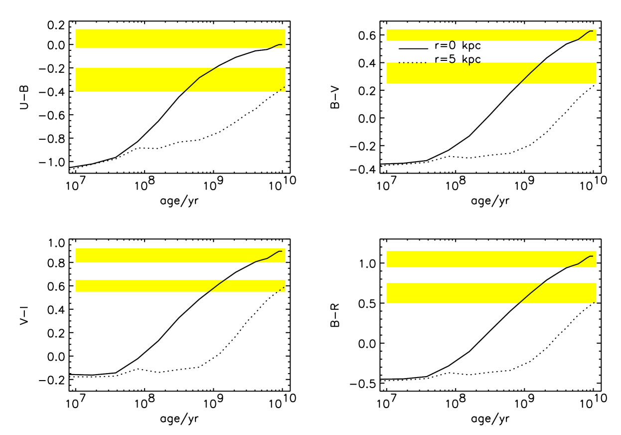
Figure 11: Time evolution for several colours predicted by our models. Two radii are shown: the nucleus (solid line) and the outermost radius of the disk (dotted line). The shaded regions are the observed values for the bluest galaxies in ? with 1$\sigma$ errors. In all cases the best fit is at late epochs ($>7$ Gyr), what shows that LSBs are not young galaxies.

4 Chemical Evolution Models

Most synthetic stellar population codes do not account for the chemical time-evolution of the stellar population, and use a simple analytical prescription for the star formation rate (e.g. the Hubble sequence is often explained like a convolution of SSPs with constant metallicity (solar) and an exponentially decaying star formation rate with different e-folding times). This approach is not self–consistent, but it has been historically used because of the lack of theoretical libraries of stellar photospheres of non–solar composition. Indeed, the way to proceed is to use chemical evolution models where $Z(t)$ and $SFR(t)$ are consistent with each other. The model of chemical evolution we use is similar to that described in ? developed to calculate the chemical evolution of the Milky Way. The main assumptions of the model are:

• The disk is represented by several circular concentric shells 2 kpc wide and no exchange of gas between them is allowed.

• The disk is formed by infall of primordial material and the infall rate is higher in the center than in the outermost regions of the disk. In particular, the infall law is expressed as:

  $$\dot{\Sigma}_{inf}(r,t)\,=\,A(r)X^{i}_{inf}e^{-t/\tau(r)}$$ (15)

  where $\tau(r)$ is the timescale for the formation of the disk at a radius $r$. The values of $\tau(r)$ are chosen in order to fit the present time radial distribution of the gas surface density in the disk. In analogy with what is required for the disk of the Milky Way, we assumed an “inside-out” mechanism of formation of such galaxies, implying that $\tau(r)$ is increasing towards larger radii (see Table 2). $X^{i}_{inf}$ is the abundance of element $i$ in the infalling gas and the chemical composition is assumed to be primordial. The parameter $A(r)$ is obtained by requiring the surface density now to be $\Sigma(r,t_{now})$, given by the disk model described in section 2:

  $$A(r)={\Sigma(r,t_{now})\over\tau(1-e^{-t_{now}/\tau(r)})}$$ (16)

• The IMF is taken from ? and is assumed to be constant in space and time.

• The star formation rate is assumed to depend on both the gas surface density, $\Sigma_{gas}(r,t)$ and the total mass surface density, $\Sigma(r,t)$. In particular, we adopted a law of the type:

  $$\psi(r,t)=\nu\Sigma_{gas}(r,t)^{k_{1}}\Sigma(r,t)^{k_{2}}$$ (17)

  with $k_{1}=1.5$ and $k_{2}=0.5$. This choice is the best for the disk of our galaxy (?; ?). The parameter $\nu$, which represents the efficiency of star formation (the inverse of the time scale for star formation) has been assumed to be $\nu_{lsb}=0.25Gyr^{-1}$.

The effect of stellar winds and outflows is properly accounted for using the energy output due to supernovae. Therefore, at each ring the model accounts for the possibility of outflow of gas due to the fact that the temperature of the interstellar gas is heated enough so the velocity of the gas becomes larger than the scape velocity.

The evolution of several chemical species (H, D, He, C, N, O, Ne, Mg, Si, S, Ca, Fe and Zn), as well as the global metallicity $Z$, is followed by taking into account detailed nucleosynthesis prescriptions by including the contributions to galactic chemical enrichment by stars of all masses. The instantaneous recycling approximation was relaxed and the stellar lifetimes were taken into account (for the basic equations see ?).

Figure 12: Area weighted colours for ? sample compared with our model predictions. Also plotted the region where colours correspond to ages larger than 7 Gyr. It transpires from the figure that LSBs have ages in excess of 7 Gyr. Of special interest is the $B-I$ $vs$ $B-R$ plot: it shows a good correlation because it samples the old stellar population and is not contaminated by recently formed stars like $U$.

In particular, we adopted the ? stellar yields for low and intermediate mass stars ($0.8\leq M/M_{\odot}\leq 8$) which produce mostly ${}^{4}He$, ${}^{12}C$, ${}^{13}C$ and ${}^{14}N$. Newer stellar yields for this range of masses are now available (?) but they do not differ significantly from the ? ones (Matteucci et al., in preparation). For the yields of $\alpha$-elements and Fe in massive stars ($M>10M_{\odot}$) we adopted the yields of ? and for type Ia supernovae (SNe) those of ?. Type Ia SNe are assumed to be the outcoming of exploding white dwarfs in binary systems and their contribution to galactic chemical evolution is computed in the way described in ?. They produce mostly Fe and some traces of $\alpha$-elements. For the yields of Zn we assumed the prescriptions given in ? where this element is assumed to originate partly from s-processing in massive stars (weak component), partly from r-processing in low mass stars (main component) and mostly from explosive nucleosynthesis in SNe of type Ia.

We computed the evolution of a disk with total final mass $M_{d}=10^{10}M_{\odot}$, $\Omega_{b}=0.05$, $\Omega_{o}=1$ and $\lambda=0.03$ and 0.06 (see Table 2).

$r/kpc$	$\frac{\Sigma}{M_{\odot}pc^{-2}}$	$\tau/Gyr$	$Z/Z_{\odot}$	$\frac{\Sigma_{\rm gas}}{M_{\odot}pc^{-2}}$
0.0	210	0.05	2.70	1.8
1.2	28	1.0	1.45	2.57
2.5	3.86	4.0	0.60	1.2
4.3	0.19	8.0	0.50	0.063
0.0	52.68	0.05	2.35	0.79
2.5	7.13	4.0	0.55	2.56
4.0	2.62	8.0	0.45	0.96
5.0	0.13	12.0	0.30	0.04

Table 2: Values for the initial surface density ($\Sigma$), $\tau$, final metallicity ($Z$) and final surface density of the gas $\Sigma_{\rm gas}$ for the two disc models considered in this work: $\lambda=0.03$ (top panel) and 0.06 (bottom panel).

5 The Model Galaxy

Using the method described in the three previous sections, we have computed colours and metallicities for the two models described in Table 2. We have assumed a halo formation redshift $z=0.7$, a baryon fraction $f_{b}=0.05$, a density parameter $\Omega_{0}=1.0$ and the Hubble constant $H_{0}=75$ kms^-1Mpc^-1. As we said before, we use the sample of ? to compare colors and surface brightness of our models with the observations. We also compare our predicted oxygen abundances to those measured in ?, and our predicted evolution of Zn $vs$ redshift with the data by ?.

5.1 Colour Evolution and Ages

Fig. 11 shows the time evolution of U-B, B-V, V-I and B-R colours for a model with halo mass $M=1.e10$ M_⊙, halo redshift formation $z=0.7$, and spin parameter $\lambda=0.06$. The central radii (solid line) and the outermost radii (dotted line) are plotted.

Also over-plotted as shaded regions are the mean values of U-B, B-V, V-I and B-R using F568-1, F571-5, UGC1230, F577-V1, UGC128 and UGC628 from ? for the central region and for the outermost radii (the extension of the shaded regions corresponds to the dispersion among the mean color of the galaxies). We choose this particular set of galaxies because they are the bluest in ? sample and therefore they set the most conservative constraint on the age (lowest age). Two important conclusions can be drawn from this plot: the best fit occurs in all cases for ages bigger than 7 Gyr, this happens in the nuclear region as well as in the outermost radii. Our model provides a good fit for both the nucleus and the outer radii simultaneously. It is worth mentioning that the observed colours of the nucleus are rather red, unequivocally indicating the presence of an old population in the LSBs. This has been recently confirmed by ? who have found a population of old, red stars ($B-H>3.5$), with colours similar to those of ellipticals, in a sample of LSBs.

A more interesting constraint on the age can be placed by using colour-colour plots. In this case we use the area weighted colours for the whole ? sample to compare our predictions. In Fig.12 we show the evolution of our model (area weighted) for two colour plots: $U-B$ $vs$ $B-V$ and $B-R$ $vs$ $B-I$. We have also drawn the lines where the colours correspond to ages bigger than 7 Gyr. It transpires from the plots that the observations are better fitted if LSBs are older than 7 Gyr. The observed points show a better correlation in $B-R$ $vs$ $B-I$ than in $U-B$ $vs$ $B-V$. This is because $I$ and $R$ sample much better the old stellar population than $U$. $U$ is affected by recent episodes of star formation, and this is the possible reason for the scatter in the $U-B$ $vs$ $B-V$ plot. However, there are LSBs with observed $U-B>-0.2$ and $B-V>0.5$, which give ages $>7$ Gyr, in agreement with the $B-R$ $vs$ $B-I$ age determination.

It is worth noticing that the $\lambda=0.03$ model has colours that are 0.2 redder than the $\lambda=0.06$ model with a similar time evolution.

These more sophisticated models confirm the results obtained in our previous paper (?), where we were using the most simplistic model to show that LSBs have an underlying population older than 7 Gyr.

5.2 Colour Profiles, Surface Brightness and Spectra

An interesting test for our model is to see if it can reproduce the colour profiles measured by ?. Fig.13 shows our model prediction compared with the mean colours for F568-1, F571-5, UGC1230, F577-V1, UGC128 and UGC628 from ? sample with error bars computed as the 1$\sigma$ value of the dispersion among the measured values. The agreement is in general rather good. The observed scatter in ? sample can be easily explained by small changes in the spin parameter or star formation rate.

Figure 13: Predicted colour profiles for the model considered in the text (lines) are compared with the bluest galaxies in ? sample (dots, see text). The agreement is excellent but our profiles are slightly steeper than the observed ones.

We have also computed the radial surface brightness for different times (Fig.14). We compare it with the averaged values for F571-5, UGC1230, F577-V1 and again the error bars correspond to the 1$\sigma$ value of the dispersion among the measured values. Our model is quite successful in fitting the observed surface brightness gradients. There is little evolution with time in the surface brightness after 7 Gyr, while the model is definitely brighter than the observed galaxies, for ages smaller than 5 Gyr.

Fig.15 and 16 show the predicted spectra for six different ages in the nuclear region (Fig.15) and in the outermost radius (Fig.16).

Figure 14: The surface brightness profiles for our model at different ages are compared to the corresponding averaged LSB from ? sample (see text). It is clear that our model gives a good fit both for the profile and the absolute value of the surface brightness in both bands. It also transpires from the figure that ages as low as 4 Gyr do not provide a good fit, reinforcing the old age argument presented in this work.

5.3 Chemical Abundances

Figure 15: Predicted spectra for the nucleus of a typical LSB.

Figure 16: Predicted spectra for the outermost radius of a typical LSB.

In the previous sections we have shown that the first stars in LSBs formed about 8-9 Gyr ago. One observable which can potentially cast doubt on the model is the metal abundance, for example the Zinc measurements of ?. In order to ensure that the metal abundance is not overpredicted, we present an illustrative computation which is designed to maximise the predicted abundance. We assume a halo collapse at $z=4$, corresponding to a look-back time of 8 Gyr if $H_{0}=75$ km s^-1 Mpc^-1. This extreme collapse redshift would correspond to rare high-peak fluctuations (e.g. ?), and leads to high surface densities, high infall rates and, of course, an early build-up of metals. It should therefore be regarded as providing a practical upper limit to the elemental abundances computed in this section.

Using our chemical evolution model it is possible to predict the evolution with radius and redshift for most chemical species. In this section we compare the prediction of our model with two samples. ? has observed HII regions in a sample of LSBs and derived their oxygen abundance. Most of the HII regions are located in the outermost part of the spiral arms. He finds quite a spread in oxygen abundance among LSBs, with a clear peak at about $[O/H]=-0.9$ and dispersion 0.15 (FWHM). His measures also show a tentative peak at about $[O/H]=-0.4$, but as is said in ?, it is partly an artifact of the method employed to determine the oxygen abundances and not a definitive feature of bimodality. In Fig.17 (upper-left panel) we show our model predictions for four radii and also show the range of oxygen abundances measured by ? as thick horizontal solid lines. It is clear that our model is consistent with the ? measures, but does not explain the lowest abundances measured by ?. This may be explained by the fact that the outermost radius is always close to (or below) the Toomre/Kennicutt threshold and it is therefore likely that some HII regions will be forming stars in areas of the galaxy with metallicity close to primordial values, while the average metallicity of the galaxy at that radius (that is what we compute) will be higher. In fact, this is well supported by the fact that the colour profiles from the sample by ? always show redder colours in the outermost radius than the ones corresponding to a galaxy with $[O/H]$ as low as $-1.2$. For the outermost radius our model predicts $[O/H]=-0.8$ in excellent agreement with the peak found by ?. It should be also noted that none of the innermost radii in our model reproduces ? measures, in good agreement with the well known fact that HII regions are usually in the outermost parts of the hosting galaxy.

Another important prediction of our model is the evolution of Zn. The right-upper panel of Fig.18 shows the predicted evolution of Zn for four different radii in our model. We also show as diamonds the data for Damped Lyman-$\alpha$ (DLA) systems observed by ?, including some upper limits. While it is difficult to establish a correlation of Zn $vs$ redshift, it transpires from the figure that the predicted Zn abundance for LSBs at different radii is consistent with the ? data. In fact the spread found at every redshift is consistent with the spread in Zn abundance predicted for LSBs. It should be noted though, that this does not mean that DLAs are LSBs, this only means that due to their old age and their presence at high-$z$, some DLAs could be caused by LSBs in the line of sight. Indeed, at least one DLA has been identified as a LSB galaxy (?).

Notice that the results derived in this section are robust for $z=0$ regardless of the formation redshift adopted for LSBs since the evolution of the chemical elements with time is very weak after the first 4 Gyr.

6 Discussion and Conclusions

6.1 The Nature of LSBs

Figure 17: The redshift evolution for some elements is plotted. The top-left panel shows the evolution of $[O/H]$ and is compared with ? measures. Our model reproduces perfectly the peak in $[O/H]$ among LSBs found by ? at $[O/H]=-0.9$. The top-right panel shows the analogous to the previous one but for $[Zn/H]$ compared with ? measures. It transpires from the figure that the predicted $[Zn/H]$ for LSBs is consistent with the spread found for DLAs.

In this work we have shown that the photometric properties of the bluest galaxies in the sample by ? can be reproduced assuming that they form and evolve as normal disk galaxies, with relatively high spin parameter. That the spin parameter alone could explain the low surface brightness was already shown by ?, but they assumed a given $M/L$ ratio. Here we have strengthened the point by also explaining the colours, the colour gradients, and the chemical abundances. We have also provided synthetic spectra that could be compared with the observations, in the effort to prove that LSB disk galaxies are indeed normal galaxies with high spin parameter. The stellar populations of LSBs are rather evolved, especially in the central part of their disks. Even the bluest galaxies in the LSB sample by ? are older than 7 Gyr, and typically star formation in these galaxies starts about 9 Gyr ago. This confirms the results of ?, where the galaxies in the same sample were found to be at least 7 Gyr old.

LSB and HSB disks are therefore hosted in similar dark matter halos that differ only for their spin parameter, and they evolve in a similar way, apart from the fact that LSB disks are less concentrated than HSB disks. This means that the present day (or low redshift) abundance of LSBs relative to HSBs should be about the same at any redshift. Moreover, the conclusions about the epoch of star formation and halo formation (see the next section), and about the colour evolution must be valid for disk galaxies in general. In particular, Fig. 11 shows that the colour evolution of LSBs is very strong. The U-B, B-V and V-I colours of the central part of the disk at high redshift are about 1 mag bluer than they are at low redshift, and the B-R colour even 1.5 mag bluer. This must be a property of disks in general, and not only of LSB disks.

6.2 Star Formation and Galaxy Formation

We have shown in section 2.1 that the size of LSB disk galaxies is such that their halos are formed in the redshift range $0.1<z<1.2$. We have also been able to estimate the formation redshift of the halo of each galaxy in the sample, and we have found a mean value $z=0.7$. In an Einstein–de–Sitter universe with $H_{0}=75$ kms^-1Mpc^-1, a redshift $z=0.7$ corresponds to a look–back time of $6.8$ Gyr. On the other hand, the photometric properties of LSB galaxies, in particular their colours, are such that star formation must have started approximately $9$ Gyr. Therefore, the star formation starts about 2 Gyr before the galactic halos are formed. These numbers are likely to be similar for HSB disk galaxies too, since they have colours and sizes very similar to LSBs, also suggesting a rather low formation redshift for their halos.

The discrepancy between the epoch when star formation starts in a galaxy and the epoch when the halo forms means that the process of star formation starts before the galactic halo has assembled, as predicted for example by bottom–up galaxy formation scenarios, characterized by power spectra with more power on sub–galactic scales than on galactic ones.

In Fig. 18 we show the evolution with redshift of the SFR. The upper panel shows the fraction of gas with time that is converted into stars at every redshift for the nucleus and the disk. The continuous thick line shows the average of the nucleus and the disk as a representative of the whole LSB. It is worth noticing that most of the gas in the nucleus is converted into stars between $2<z<4$, while most of the star formation in the disk takes place at $z<2$. The lower panel shows the global SFR in the Universe for LSBs assuming that they have the same comoving number density as HSBs and that the typical mass for a $L_{*}$ LSB is a factor 5 smaller than the typical mass of a normal $L_{*}$ galaxy. The data points are taken from ? and trace the global SFR in the Universe for HSBs. LSBs lie below the observed points because they have typical masses smaller than HSBs. The important point to notice here is that the global SFR for LSBs has a flatter evolution than the observed points.

Figure 18: Top panel shows the gas fraction with time in our LSB model that is converted into stars $vs$ redshift for the disk and the nucleus. The thick line corresponds to the average of the nucleus and the disk and should be a fair representative of the whole LSB. The bottom panel shows the predicted global SFR in the Universe due to LSBs assuming that the mass for a $L_{*}$ LSB is 5 smaller than the mass for a $L_{*}$ HSB and that the comoving number density for LSBs is the same as for HSBs (see text). The observed points are taken from ?. Notice that the evolution with redshift is flatter than the one measured by ?.

6.3 Discussion

In order to explain the rotational properties of LSBs, we require halos with velocity dispersions $\approx 100$ km s^-1, or masses $\approx 10^{11}$ M_⊙. This is also consistent with the required gas masses and a baryon fraction of a few percent. To obtain the right sizes of LSBs, we additionally require a relatively late halo collapse, $z\simeq 0.7$. Clearly this may present a problem for galaxy formation models which have a lot of power on the appropriate scale. An obvious example is COBE-normalised CDM, with shape parameter $\Gamma=0.5$ (?), for which the characteristic collapse redshift for $100$ km s^-1 halos is around $z=6$. Reducing the amplitude to that of standard CDM (bias parameter 2.5) alleviates the problem to a certain extent, but the collapse redshift is still $z=3$. It is more promising to consider mixed dark matter models, for which the power spectrum is in any case a better match to the observed galaxy spectrum. For a neutrino fraction of 30%, the comoving number density of halos with mass exceeding $1.5\times 10^{11}$ M_⊙ reaches 0.01 $h^{3}$ Mpc^-3, comparable to the density of large galaxies, at a redshift of about 1.7 ?. This is still a little high, but it should be remembered that the collapse of halos of given mass does take place over a reasonably wide range of redshifts, and some fraction of halos would form after $z=0.7$. In the model considered by ?, about a quarter of halos exceeding this mass form after $z=0.7$. Analytically, there is expected to be a weak correlation between high spin and late collapse ?, and numerical simulations by ? show an anticorrelation between spin and density.

We postulate therefore that the LSBs form in halos with high spin which form relatively late, in the context of a hierarchical model. The indications are that a model with relatively little small-scale power, such as mixed dark matter, would do best here, but there are enough uncertainties in the collapse redshift, both in the simplifications of the halo model, and in physical processes which might delay collapse (e.g. ?) that this conclusion is not strong.

In summary, the most important results of this work are:

1. Observed colour profiles, chemical abundances and surface brightness profiles for LSBs are well fitted if they are assumed to have a spin parameter for its halo higher than HSBs.

2. LSBs are not young objects, as often claimed in the literature, since their colours are well fitted by old ($>7$ Gyr) stellar populations.

3. There is discrepancy between the photometric age of the galaxies and the age of formation of their halo, which indicates that star formation can start about 2 Gyr before the halo is formed. This is perfectly acceptable in hierarchical models of galaxy formation, and, as discussed in the text, the discrepancy can be reduced or removed if the cosmological model we have assumed is incorrect. If an open ($\Lambda$) cosmology had been adopted, the above discrepancy would have been completely removed.

References

- [Babul & Rees¡1992¿] Babul A., Rees M. J., 1992. MNRAS, 255, 346.
- [Cole et al.¡1994¿] Cole S., Aragon-Salamanca A., Frenk C. S., Navarro J. F., Zepf S. E., 1994. MNRAS, 271, 781.
- [Dalcanton, Spergel & Summers¡1997¿] Dalcanton J. J., Spergel D. N., Summers F. J., 1997. ApJ, 482, 659.
- [De Blok & McGaugh¡1997¿] De Blok W. J. G., McGaugh S. S., 1997. MNRAS, 290, 533.
- [De Blok, McGaugh & Van Der Hulst¡1996¿] De Blok W. J. G., McGaugh S. S., Van Der Hulst J. M., 1996. MNRAS, 283, 18.
- [De Blok, Van Der Hulst & Bothun¡1995¿] De Blok W. J. G., Van Der Hulst J. M., Bothun G. D., 1995. MNRAS, 274, 235.
- [Dunlop et al.¡1996¿] Dunlop J., Peacock J., Spinrad H., Dey A., Jimenez R., Stern D., Windhorst R., 1996. Nature, 381, 581.
- [Fall & Efstathiou¡1980¿] Fall S. M., Efstathiou G., 1980. MNRAS, 193, 189.
- [Freeman¡1970¿] Freeman K. C., 1970. ApJ, 160, 811.
- [Frenk & White¡1991¿] Frenk C. S., White S. D. M., 1991. ApJ, 379, 52.
- [Frenk et al.¡1985¿] Frenk C. S., White S. D. M., Efstathiou G., Davis M., 1985. Nature, 317, 595.
- [Frenk et al.¡1988¿] Frenk C. S., White S. D. M., Davis M., Efstathiou G., 1988. ApJ, 327, 507.
- [Gunn & Gott¡1972¿] Gunn J., Gott R., 1972. ApJ, 176, 1.
- [Heavens & Peacock¡1988¿] Heavens A. F., Peacock J. A., 1988. MNRAS, 232, 339.
- [Impey, Bothun & Malin¡1988¿] Impey C., Bothun G., Malin D., 1988. ApJ, 330, 634.
- [Irwin et al.¡1990¿] Irwin M. J., Davies J. I., Disney M. J., Phillipps S., 1990. MNRAS, 245, 289.
- [Jimenez et al.¡1997¿] Jimenez R., Heavens A., Hawkins M., Padoan P., 1997. MNRAS, 292, L5.
- [Jimenez et al.¡1998¿] Jimenez R., Dunlop J., Peacock J., MacDonald J., Jorgensen U., 1998. MNRAS, submitted.
- [Kauffmann, White & Guiderdoni¡1993¿] Kauffmann G., White S. D. M., Guiderdoni B., 1993. MNRAS, 264, 201.
- [Kennicutt¡1989¿] Kennicutt R. C., 1989. ApJ, 344, 685.
- [Klypin et al.¡1995¿] Klypin A., Borgani S., Holtzman J., Primack J., 1995. ApJ, 444, 1.
- [Kurucz¡1992¿] Kurucz R., 1992. CDROM13, .
- [Madau¡1997¿] Madau P., 1997. astro-ph/9709147, .
- [Matteucci & Francois¡1989¿] Matteucci F., Francois P., 1989. MNRAS, 239, 885.
- [Matteucci & Greggio¡1986¿] Matteucci F., Greggio L., 1986. A&A, 154, 279.
- [Matteucci et al.¡1993¿] Matteucci F., Raiteri C. M., Busson M., Gallino R., Gratton R., 1993. A&A, 272, 421.
- [Matteucci¡1986¿] Matteucci F., 1986. PASP, 98, 973.
- [McGaugh & Bothun¡1994¿] McGaugh S. S., Bothun G. D., 1994. AJ, 107, 530.
- [McGaugh, Bothun & Schombert¡1995¿] McGaugh S. S., Bothun G. D., Schombert J. M., 1995. AJ, 110, 573.
- [McGaugh¡1994¿] McGaugh S. S., 1994. ApJ, 426, 135.
- [Mo, Mao & White¡1997¿] Mo H. J., Mao S., White S. D. M., 1997. astro-ph/9707093, .
- [Mo, McGaugh & Bothun¡1994¿] Mo H. J., McGaugh S. S., Bothun G. D., 1994. MNRAS, 267, 129.
- [Navarro, Frenk & White¡1997¿] Navarro J. F., Frenk C. S., White S. D. M., 1997. ApJ, 490, 493.
- [Padoan, Jimenez & Antonuccio-Delogu¡1997¿] Padoan P., Jimenez R., Antonuccio-Delogu V., 1997. ApJ, 481, 27L.
- [Peacock & Heavens¡1985¿] Peacock J. A., Heavens A. F., 1985. MNRAS, 217, 805.
- [Pettini et al.¡1997¿] Pettini M., Smith L. J., King D. L., Hunstead R. W., 1997. ApJ, 486, 665.
- [Quillen & Pickering¡1997¿] Quillen A. C., Pickering T. E., 1997. astro-ph/9705115, .
- [Quinn, Salmon & Zurek¡1986¿] Quinn P. J., Salmon J. K., Zurek W. H., 1986. Nature, 322, 329.
- [Renzini & Voli¡1981¿] Renzini A., Voli M., 1981. A&A, 94, 175.
- [Scalo¡1986¿] Scalo J. M., 1986. Fundamentals of Cosmic Physics, 11, 1.
- [Spinrad et al.¡1997¿] Spinrad H., Dey A., Stern D., Dunlop J., Peacock J., Jimenez R., Windhorst R., 1997. ApJ, 484, 581.
- [Sprayberry et al.¡1997¿] Sprayberry D., Impey C. D., Irwin M. J., Bothun G. D., 1997. ApJ, 482, 104.
- [Sprayberry, Impey & Irwin¡1996¿] Sprayberry D., Impey C. D., Irwin M. J., 1996. ApJ, 463, 535.
- [Steidel et al.¡1994¿] Steidel C. C., Pettini M., Dickinson M., Persson S. E., 1994. AJ, 108, 2046.
- [Thielemann, Nomoto & Hashimoto¡1996¿] Thielemann F.-K., Nomoto K., Hashimoto M.-A., 1996. ApJ, 460, 408.
- [Toomre¡1964¿] Toomre A., 1964. ApJ, 139, 1217.
- [Tosi¡1982¿] Tosi M., 1982. ApJ, 254, 699.
- [Ueda et al.¡1994¿] Ueda H., Shimasaku K., Suginohara T., Suto Y., 1994. PASJ, 46, 319.
- [Van Den Hoek & Groenewegen¡1997¿] Van Den Hoek L. B., Groenewegen M. A. T., 1997. Astronomy and Astrophysics Supplement Series, 123, 305.
- [Van Der Hulst et al.¡1993¿] Van Der Hulst J. M., Skillman E. D., Smith T. R., Bothun G. D., McGaugh S. S., De Blok W. J. G., 1993. AJ, 106, 548.
- [Woosley & Weaver¡1995¿] Woosley S. E., Weaver T. A., 1995. ApJs, 101, 181.
- [Zwaan et al.¡1995¿] Zwaan M. A., Van Der Hulst J. M., De Blok W. J. G., McGaugh S. S., 1995. MNRAS, 273, L35.