Computing CMB anisotropy in Compact Hyperbolic spaces

Abstract

The measurements of CMB anisotropy have opened up a window for probing the global topology of the universe on length scales comparable to and beyond the Hubble radius. For compact topologies, the two main effects on the CMB are: (1) the breaking of statistical isotropy in characteristic patterns determined by the photon geodesic structure of the manifold and (2) an infrared cutoff in the power spectrum of perturbations imposed by the finite spatial extent. We present a completely general scheme using the regularized method of images for calculating CMB anisotropy in models with nontrivial topology, and apply it to the computationally challenging compact hyperbolic topologies. This new technique eliminates the need for the difficult task of spatial eigenmode decomposition on these spaces. We estimate a Bayesian probability for a selection of models by confronting the theoretical pixel-pixel temperature correlation function with the cobe–dmr data. Our results demonstrate that strong constraints on compactness arise: if the universe is small compared to the ‘horizon’ size, correlations appear in the maps that are irreconcilable with the observations. If the universe is of comparable size, the likelihood function is very dependent upon orientation of the manifold wrt the sky. While most orientations may be strongly ruled out, it sometimes happens that for a specific orientation the predicted correlation patterns are preferred over the conventional infinite models.

1 Introduction

The remarkable degree of isotropy of the cosmic microwave background (CMB) points to homogeneous and isotropic Freidmann-Robertson-Walker (FRW) models for the universe. The underlying Einstein’s equations of gravitation are purely local, completely unaffected by the global topological structure of space-time. In fact, in the absence of spatially inhomogeneous perturbations, a FRW model predicts an isotropic CMB regardless of the global topology.

The observed large scale structure in the universe implies spatially inhomogeneous primordial perturbations exist which gave rise to the observed anisotropy of the CMB. The global topology of the universe does affect the local observable properties of the CMB anisotropy. In compact universe models, the finite spatial size usually precludes the existence of primordial fluctuations with wavelengths above a characteristic scale related to the size of the universe. As a result, the power in the CMB anisotropy is suppressed on large angular scales. Another consequence is the breaking of statistical isotropy in characteristic patterns determined by the photon geodesic structure of the manifold. One can search for such patterns statistically in the COBE maps, and to the extent that they are not there, one can constrain the size of the universe and its topology.

Much recent astrophysical data suggest the cosmological matter density parameter, $\Omega_{0}$, is subcritical [1]. If a (possibly varying) cosmological constant is absent or insufficient to bring the total density to the critical value, this would imply a hyperbolic spatial geometry for the universe (commonly referred to as the ‘open’ universe in the cosmological literature). The topologically trivial (simply connected) hyperbolic 3-space, ${\cal H}^{3}$, is non-compact and has infinite size. There are numerous theoretical motivations, however, to favor a spatially compact universe [2]. To reconcile a compact universe with a flat or hyperbolic geometry, consideration of spaces with non trivial topology (non simply connected spaces) is required. A compact cosmological model can be constructed by identifying points on the standard infinite flat or hyperbolic FRW spaces by the action of a suitable discrete subgroup, $\Gamma$, of the full isometry group, $G$, of the FRW space. The infinite FRW spatial hypersurface is the universal cover, tiled by copies of the compact space (most appropriately represented as the Dirichlet domain with the observer at its basepoint). Any point ${{\bf x}}$ of the compact space has an image ${{\bf x}}_{i}=\gamma_{i}{{\bf x}}$ in each copy of the Dirichlet domain on the universal cover, where $\gamma_{i}\in\Gamma$.

The hyperbolic manifold, ${\cal H}^{3}$, can be viewed as a hyperbolic section embedded in four dimensional flat Lorentzian space. The isometry group of ${\cal H}^{3}$ is the group of rotations in the four space – the proper Lorentz group, $SO(3,1)$. A compact hyperbolic (CH) manifold is then completely described by a discrete subgroup, $\Gamma$, of the proper Lorentz group, $SO(3,1)$. The Geometry Centre at the University of Minnesota has a large census of CH manifolds and public domain software SnapPea [3]. We have adapted this software to tile ${\cal H}^{3}$ under a given topology using a set of generators of $\Gamma$. The tiling routine uses the generator product method and ensures that all distinct tiles within a specified tiling radius are obtained.

A CH manifold, ${\cal M}$, is characterized by a dimensionless number, ${\cal V}_{\!\cal M}\equiv V_{\!\cal M}/d_{c}^{3}$, where $V_{\!\cal M}$ is the volume of the space and $d_{c}$ is the curvature radius [4]. There are a countably infinite number of CH manifolds with no upper bound on ${\cal V}_{\!\cal M}$. The smallest CH manifold discovered so far has ${\cal V}_{\!\cal M}=0.94$ [5].   The Minnesota census lists several thousands of these manifolds with ${\cal V}_{\!\cal M}$ up to $\sim 7$. In the cosmological context, the physical size of the curvature radius $d_{c}$ is determined by the density parameter and the Hubble constant $H_{0}$: $d_{c}=(c/H_{0})/\sqrt{1-\Omega_{0}}$. The physical volume of the CH manifold with a given topology, i.e., a fixed value of $V_{\!\cal M}/d_{c}^{3}$, is smaller for smaller values of $\Omega_{0}$. Two quantities which characterize linear dimensions of the Dirichlet domain are $R_{>}$ and $R_{<}$, the radii of circumscribing and inscribing spheres, respectively.

In the standard picture, the CMB that we observe is a Planckian distribution of relic photons which decoupled from matter at a redshift $\approx 1100$. These photons have freely propagated over a distance $R_{\sc ls}\approx 2d_{c}\,{\rm arctanh}\sqrt{1-\Omega_{0}}$, comparable to the “horizon” size. For the adiabatic fluctuations we consider here, the dominant contribution to the anisotropy in the CMB temperature measured with wide-angle beams ($\theta_{\sc fwhm}\mathrel{\hbox to0.0pt{\lower 3.0pt\hbox{$\mathchar 536\relax$}\hss}\raise 2.0pt\hbox{$\mathchar 318\relax$}}2^{\circ}\Omega_{0}^{1/2}$) comes from the cosmological metric perturbations through the Sachs-Wolfe effect.

The adiabatic cosmological metric perturbations can be expressed in terms of a scalar gravitational potential, $\Phi({\bf x},\tau)$. The dynamical equation for the gravitational potential allows for separation of the spatial and temporal dependence, $\Phi({\bf x},\tau)=F(\tau)\Phi({\bf x},\tau_{\sc ls})$, where $F(\tau)$ encodes the time dependence of the metric perturbations and $\Phi({\bf x},\tau_{\sc ls})$ is the field configuration on the three-hypersurface of constant time $\tau=\tau_{\sc ls}$ when the last scattering of CMB photons took place. We shall study open, $\Omega_{0}<1$, models with zero cosmological constant where in the matter dominated phase, [8]

$$F(\tau)=\frac{5(\sinh^{2}\tau-3\tau\sinh\tau+4\cosh\tau-4)}{(\cosh\tau-1)^{3}}\,.$$ (1)

Here and further on we use dimensionless conformal time $\tau$ expressed in units of the curvature radius. A non-zero cosmological constant can be trivially incorporated in our analysis by using the appropriate solution for $F(\tau)$.

We write the Sachs-Wolfe formula for the CMB temperature fluctuation, $\Delta T(\hat{q})$, in a direction $\hat{q}$, in the form

$$\frac{\Delta T}{T}(\hat{q})=\frac{1}{3}\Phi(\hat{q}{\chi_{\!{}_{\rm H}}},\tau_{\sc ls})+2\int_{0}^{\chi_{\!{}_{\rm H}}}d\chi f(\chi)\Phi(\hat{q}\chi,\tau_{\sc ls})\,,\quad f(\chi)=\frac{d}{d\tau}F(\tau)\bigg{|}_{\tau={\chi_{\!{}_{\rm H}}}-\chi}\,,$$ (2)

where $\chi$ is the affine parameter along the photon path from $\chi=0$ at the observer position to ${\chi_{\!{}_{\rm H}}}=R_{\sc ls}/d_{c}$. The first term is called the surface or “naive” Sachs-Wolfe effect (NSW). The second term, which is nonzero only if $\Phi$ varies with time between $\tau_{\sc ls}$ and now, is the integrated Sachs-Wolfe effect (ISW). The angular correlation between the CMB temperature fluctuations in two directions in the sky is then given by

$$C(\hat{q},\hat{q}^{\prime})\equiv\left\langle\frac{\Delta T}{T}(\hat{q})\frac{\Delta T}{T}(\hat{q}^{\prime})\right\rangle=\frac{1}{9}\langle\Phi(\hat{q}{\chi_{\!{}_{\rm H}}},\tau_{\sc ls})\Phi(\hat{q}^{\prime}{\chi_{\!{}_{\rm H}}},\tau_{\sc ls})\rangle$$

$$\hbox to0.0pt{\hss${}+{}$}\frac{2}{3}\int_{0}^{\chi_{\!{}_{\rm H}}}d\chi~{}f(\chi)~{}\left[\langle\Phi(\hat{q}\chi,\tau_{\sc ls})\Phi(\hat{q}^{\prime}{\chi_{\!{}_{\rm H}}},\tau_{\sc ls})\rangle+\langle\Phi(\hat{q}^{\prime}\chi,\tau_{\sc ls})\Phi(\hat{q}{\chi_{\!{}_{\rm H}}},\tau_{\sc ls})\rangle\right]$$

$$\hbox to0.0pt{\hss${}+{}$}4\int_{0}^{\chi_{\!{}_{\rm H}}}d{\chi_{\!{}_{\rm 1}}}~{}f({\chi_{\!{}_{\rm 1}}})~{}\int_{0}^{\chi_{\!{}_{\rm H}}}d{\chi_{\!{}_{\rm 2}}}~{}f({\chi_{\!{}_{\rm 2}}})~{}\langle\Phi(\hat{q}{\chi_{\!{}_{\rm 1}}},\tau_{\sc ls})\Phi(\hat{q}^{\prime}{\chi_{\!{}_{\rm 2}}},\tau_{\sc ls})\rangle\,.$$ (3)

The main point to be noted is that $C(\hat{q},\hat{q}^{\prime})$ depends on the spatial two point correlation function, $\xi_{\Phi}\equiv\langle\Phi({\bf x},\tau_{\sc ls})\Phi({\bf x^{\prime}},\tau_{\sc ls})\rangle$ of $\Phi$ on the three-hypersurface of last scattering. This is due to the fact that the equation of motion for $\Phi$ allows a separation of spatial and temporal dependence.

Although in this work we restrict our attention to the Sachs-Wolfe effect which dominates when the beam size is large, we should point out that other effects which contribute to the CMB anisotropy at finer resolution can also be approximated in terms of spatial correlation of quantities defined on the hypersurface of last scattering [9].

2 Method of Images

As described in the previous section, the angular correlation function for the CMB temperature anisotropy can be expressed in terms of the two point spatial correlation function $\xi_{\Phi}({\bf x},{\bf x}^{\prime})$ for the gravitational potential field, $\Phi({\bf x},\tau_{\sc ls})$ defined on the three-hypersurface of last scattering. The correlation function $\xi_{\Phi}$ can be expressed formally in terms of the eigenfunctions, $\Psi_{i}$ of the Laplace operator, $\nabla^{2}$, on the hypersurface (with positive eigenvalues $k_{i}^{2}\geq 0$), as [8, 10]

$$\xi_{\Phi}({\bf x},{\bf x}^{\prime})=\sum_{i}\Psi_{i}({\bf x})\Psi_{i}^{*}({\bf x}^{\prime})P_{\Phi}(k_{i})\,,\ {\rm where}\ (\nabla^{2}+k_{i}^{2})\Psi_{i}=0\,.$$ (4)

The function $P_{\Phi}(k_{i})$ is the initial power spectrum of the gravitational potential.

In order to calculate the $\xi_{\Phi}$ on CH manifolds we have developed the method of images [11] which evades the difficult problem of solving for eigenfunctions of the Laplacian on these manifolds and, in general, on any nonsimply connected manifold, ${\cal M}$. The manifold ${\cal M}$ can be regarded as a quotient of a simply connected manifold ${\cal M}^{u}$ by a fixed point free discontinuous subgroup $\Gamma$ of the isometry group of ${\cal M}^{u}$, i.e., ${\cal M}={\cal M}^{u}/\Gamma$. The manifold ${\cal M}^{u}$ is referred to as the universal cover of ${\cal M}$. The elements $\gamma\in\Gamma$ produce images of the manifold ${\cal M}$ which tessellate ${\cal M}^{u}$.

The spectrum of the Laplacian on a compact space (thus with closed boundary conditions) is a discrete ordered set of eigenvalues $\{k^{2}_{i}\}$ ($k_{0}^{2}=0$ and $k_{i}^{2}\leq k^{2}_{i+1}$, with multiply repeated eigenvalues counted separately). The set $\{\Psi_{i}\}$ is the corresponding complete orthonormal set of eigenfunctions on ${\cal M}$. The eigenfunctions $\Psi_{i}$ on ${\cal M}$ are also eigenfunctions on the universal cover, ${\cal M}^{u}$. As a result these eigenfunctions simultaneously satisfy the integral equations for the correlation functions in both ${\cal M}^{u}$ and ${\cal M}$,

$$\int_{{\cal M}^{u}}d{\bf x^{\prime}}~{}\xi^{u}_{\Phi}({\bf x},{\bf x}^{\prime})~{}\Psi_{i}({\bf x}^{\prime})=P_{\Phi}(k_{i})\Psi_{i}({\bf x})\,,$$ (5)

$$\int_{\cal M}d{\bf x^{\prime}}~{}\xi^{c}_{\Phi}({\bf x},{\bf x}^{\prime})~{}\Psi_{i}({\bf x^{\prime}})=P_{\Phi}(k_{i})\Psi_{i}({\bf x})\,.$$ (6)

Using the fact that the $\Psi_{i}$ are automorphic with respect to $\Gamma$ ($\Psi(\gamma{\bf x})=\Psi({\bf x}),\forall\gamma\in\Gamma$), and that ${\cal M}$ tessellates ${\cal M}^{u}$,

$$\int_{{\cal M}^{u}}d{\bf x^{\prime}}~{}\xi^{u}_{\Phi}({\bf x},{\bf x}^{\prime})\Psi_{i}({\bf x^{\prime}}) =\sum_{\gamma\in\Gamma}\int_{\cal M}d{\bf x^{\prime}}~{}\xi^{u}_{\Phi}({\bf x},\gamma{\bf x}^{\prime})~{}\Psi_{i}({\bf x^{\prime}})$$ (7)

$$=\int_{\cal M}d{\bf x^{\prime}}~{}\left[~{}\sum_{\gamma\in\Gamma}^{\prime}\xi^{u}_{\Phi}({\bf x},\gamma{\bf x}^{\prime})~{}\right]\Psi_{i}({\bf x^{\prime}}),$$

where $\sum^{\prime}$ denotes a possible need for regularization at the last step when the order of integration and summation is reversed. The regularization is achieved through a counterterm which removes the contribution of the homogeneous $k^{2}=0$ mode. Using eqs. (6) and (7) leads to the main equation of our method of images [9] expressing the correlation function on a compact space (and more generally, any non-simply connected space) as a sum over the correlation function on its universal cover calculated between ${\bf x}$ and the images $\gamma{\bf x^{\prime}}$ ($\gamma\in\Gamma$) of ${\bf x^{\prime}}$:

$$\xi^{c}_{\Phi}({\bf x},{\bf x}^{\prime}) =\sum_{\gamma\in\Gamma}^{\prime}\xi^{u}_{\Phi}({\bf x},\gamma{\bf x}^{\prime})$$ (8)

$$=\sum_{\gamma\in\Gamma}\xi^{u}_{\Phi}({\bf x},\gamma{\bf x}^{\prime})-\frac{1}{V_{\!\cal M}}\int_{{\cal M}^{u}}d{\bf x^{\prime}}~{}\xi^{u}_{\Phi}({\bf x},{\bf x}^{\prime})\,.$$

3 Compact Hyperbolic Models

For cosmological CH models, ${\cal M}^{u}\equiv{\cal H}^{3}$, the three dimensional hyperbolic (uniform negative curvature) manifold. The local isotropy and homogeneity of ${\cal H}^{3}$ implies $\xi^{u}_{\Phi}({\bf x},{\bf x}^{\prime})$ depends only on the proper distance, $r\equiv d({\bf x},{\bf x^{\prime}})$, between the points ${\bf x}$ and ${\bf x^{\prime}}$. The eigenfunctions on the universal cover are of course well known for all homogeneous and isotropic models [17]. Consequently $\xi^{u}_{\Phi}({\bf x},{\bf x}^{\prime})$ can be obtained through equation (4). The initial power spectrum $P_{\Phi}(k)$ is believed to be dictated by an early universe scenario for the generation of primordial perturbations. We assume that the initial perturbations are generated by quantum vacuum fluctuations during inflation. This leads to

$$\xi^{u}_{\Phi}({\bf x},{\bf x}^{\prime})\equiv\xi^{u}_{\Phi}(r)=\int_{0}^{\infty}\frac{d\beta~{}\beta}{(\beta^{2}+1)}~{}\frac{\sin(\beta r)}{\beta\sinh r}~{}~{}{\cal P}_{\Phi}(\beta)\,,$$ (9)

where $\beta\equiv\sqrt{(kd_{c})^{2}-1}$ and ${\cal P}_{\Phi}(\beta)\equiv\beta(\beta^{2}+1)P_{\Phi}(k)/(2\pi^{2})$ is the mean square fluctuation in $\Phi$ per logarithmic interval of $k$. We consider the simplest inflationary models, where ${\cal P}_{\Phi}(k)$ is approximately constant in the subcurvature sector ( $kd_{c}>1$). This is the generalization of the Harrison-Zeldovich spectrum in spatially flat models to hyperbolic spaces [18, 19]. Sub-horizon vacuum fluctuations during inflation are not expected to generate supercurvature modes, those with $kd_{c}<1$, which is why they are not included in eq.(9). Indeed, since $H^{2}>1/(ad_{c})^{2}$, for modes with $kd_{c}<1$ we always have $k/(aH)<1$ so inflation by itself does not provide a causal mechanism for their excitation. Moreover, the lowest non-zero eigenvalue, $k_{1}>0$ in compact spaces provides an infra-red cutoff in the spectrum which can be large enough in many CH spaces to exclude the supercurvature sector entirely ($k_{1}d_{c}>1$). (See $\S$ 4.1 and [9].) Even if the space does support supercurvature modes, some physical mechanism needs to be invoked to excite them, e.g., as a byproduct of the creation of the compact space itself, but which could be accompanied by complex nonperturbative structure as well. To have quantitative predictions for $P_{\Phi}(k)$ would require addressing this possibility in a full quantum cosmological context. We note that our main conclusions regarding peculiar correlation features in the CMB anisotropy (see $\S$ 4.2) would qualitatively hold even in the presence of supercurvature modes.

3.1 Numerical implementation of method of images

Although equation (8) encodes the basic formula for calculating the correlation function, it is not numerically implementable as is. Both the sum and the integral in equation (8) are divergent and the difference needs to be taken as a limiting process of summation of images and integration up to a finite distance $r_{*}$:

$$\xi^{c}_{\Phi}({\bf x},{\bf x}^{\prime})=\lim_{r_{*}\to\infty}\left[\sum_{r_{j}<r_{*}}\xi^{u}_{\Phi}(r_{j})-\frac{4\pi}{V_{\!\cal M}}\int_{0}^{r_{*}}dr~{}\sinh^{2}r~{}\xi^{u}_{\Phi}(r)\right],~{}~{}~{}~{}r_{j}=d({\bf x},\gamma_{j}{\bf x}^{\prime})\,.$$ (10)

The volume element in the integral corresponds to ${\cal H}^{3}$. In [9] we conduct an instructive analytical study of the regularization procedure by varying an artificial infrared cutoff.

In hyperbolic spaces, the number of images within a radius $r_{*}$ grows exponentially with $r_{*}$ and it is not numerically feasible to extend direct summation to large values of $r_{*}$. The presence of the counterterm, however, besides regularizing, significantly improves convergence. This can be intuitively understood as follows : $\xi^{u}_{\Phi}(r_{j})$ represents a sampling of a smooth function at discrete points $r_{j}$. In a distant radial interval $[r,r+dr],~{}r\gg R_{>},~{}dr\sim R_{>}$ there are approximately $(4\pi/V_{\!\cal M})~{}\sinh^{2}r~{}dr$ images. The sum, $\sum_{r_{j}}\xi^{u}_{\Phi}(r_{j})$, within this interval is similar to the (Monte-Carlo type) estimation of the integral, therefore one may approximate the sum over all distant images beyond a radius $r_{*}$ by an integral to obtain

$$\tilde{\xi}^{c}_{\Phi}({\bf x},{\bf x}^{\prime})=\sum_{r_{j}<r_{*}}\xi^{u}_{\Phi}(r_{j})+\frac{4\pi}{V_{\!\cal M}}\int_{r_{*}}^{\infty}dr~{}\sinh^{2}r~{}\xi^{u}_{\Phi}(r)\,.$$ (11)

The tilde on $\xi^{c}_{\Phi}({\bf x},{\bf x}^{\prime})$ denotes the fact that it is approximate and unregularized. Subtracting the integral $(4\pi/V_{\!\cal M})\int_{0}^{\infty}dr~{}\sinh^{2}r~{}\xi^{u}_{\Phi}(r)$ as dictated by the regularization eq.(8), we recover the finite $r_{*}$ term of the limiting sequence in eq.(10). This demonstrates that even at a finite $r_{*}$, in addition to the explicit sum over images with $r_{j}<r_{*}$, the expression for $\xi^{c}_{\Phi}$ in eq.(10) contains the gross contribution from all distant images, $r_{j}>r_{*}$. Numerically we have found it suffices to evaluate the right hand side in eq.(10) up to $r_{*}$ about $4$ to $5$ times the domain size $R_{>}$ to obtain a convergent result for $\xi^{c}_{\Phi}({\bf x},{\bf x}^{\prime})$.

After this project was completed, we learned that estimation (11) is similar to the remainder term obtained in  [20] to incorporate the gross contributions of long periodic orbits in evaluating the “Selberg trace formula”(e.g., [21]) in the quantum particle problem on 2D CH surfaces. Whereas the focus in [20] was an accurate computation of eigenvalues for determining the quantum energy levels of the classically chaotic system, our focus is on correlation function evaluation in 3D. We emphasize that it is the regularized procedure (10) following directly from eq.(8) which is central to the success of our method. The form of the unregularized correlation function, $\tilde{\xi}^{c}_{\Phi}({\bf x},{\bf x}^{\prime})$, in eq.(11) suggested by the approximate treatment of distant images discussed above, in fact, also follows from the form of the regularizing counterterm in eq.(8).

Figure 1 illustrates the steps involved in implementing the regularized method of images. The value of $\xi^{c}_{\Phi}$ as a function of $r_{*}$ has some residual jitter, which arises because of the boundary effects due to the sharp “top-hat” averaging over a spherical ball chosen for the counterterm in eq.(10). This can be smoothed out by resummation techniques [22]. We use Cesaro resummation for this purpose.

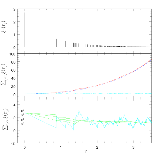
Figure 1: This illustrates the regularization of the correlation function $\xi^{c}_{\Phi}({\bf x},{\bf x}^{\prime})$. The example shown is the correlation function at zero-point separation at some point on the CH manifold m004(-5,1). The topmost panel shows the contributions to $\xi^{c}_{\Phi}({\bf x},{\bf x}^{\prime})$ from close images and the distances to the images. The upper solid curve in the middle panel shows the cumulative build up of $\sum_{r_{j}<r_{*}}\xi^{u}_{\Phi}(r_{j})$ with successive addition of distant images. The dashed curve is the regularizing counterterm required to remove the zero-mode contribution and the lower solid curve shows the cumulative value of regularized $\xi^{c}_{\Phi}({\bf x},{\bf x}^{\prime})$ which fluctuates around the true value after sufficient number of images have been added. The bottom panel demonstrates that this residual jitter ($s^{0}$) in the estimate of $\xi^{c}_{\Phi}({\bf x},{\bf x}^{\prime})$ can be removed by Cesaro resummation. The sequence of lines, $s^{1},s^{2}$& $s^{3}$ shows the result of applying first, second and third order Cesaro resummation. The accuracy at the second order is usually sufficient.

3.2 Computing the CMB anisotropy

For Gaussian perturbations, the angular correlation function, $C(\hat{q},\hat{q}^{\prime})$, completely encodes the CMB anisotropy predictions of a model. To confront observations, the celestial sphere is discretized into $N_{p}$ pixels labeled by $p$, with $N_{p}$ determined by the angular resolution of the measurements. We test the models against the four-year cobe–dmr data. The six cobe–dmr maps [23] are first compressed into a (A+B)(31+53+90 GHz) weighted-sum map, with the customized Galactic cut advocated by the DMR team, basically at $\pm 20^{\circ}$ but with extra pixels removed in which contaminating Galactic emission is known to be high, and with the dipole and monopole removed. Although one can do analysis with the map’s $(2.6^{\circ})^{2}$ pixels, this “resolution 6” pixelization of the quadrilateralized sphere is oversampled relative to the COBE beam size, and there is no effective loss of information if we do further data compression by using “resolution 5” pixels, $(5.2^{\circ})^{2}$ [24]. The celestial sphere is then represented by $N_{p}=1536$ pixels before the Galactic cut, with $N_{p}=999$ pixels remaining after the cut is made.

Full Bayesian linear comparison of the model with the data requires computation of the $N_{p}\times N_{p}$ pixel-pixel correlation matrix, $C_{Tpp^{\prime}}\equiv C(\hat{q}_{p},\hat{q}_{p^{\prime}})$. The expression for $C(\hat{q},\hat{q}^{\prime})$ in eq. (3) involves an integral along the line of sight from the observer to the surface of last scattering – the integrated Sachs–Wolfe term (ISW). We find that a simple integration rule using $N_{L}$ points along each line of sight gives accurate results when the points are spaced at equal increments of $F(\tau)$, which is determined by $\Omega_{0}$. Consequently, to get the full $C_{Tpp^{\prime}}$ matrix we need to evaluate the correlation function, $\xi^{c}_{\Phi}({\bf x},{\bf x}^{\prime})$, between $N_{p}(N_{p}+1)N_{L}^{2}/2$ pairs of points on the constant-time hypersurface of last scattering.

To calculate $C_{Tpp^{\prime}}$ in the standard infinite open cosmological models with this real-space integration to an accuracy comparable to that of the traditional evaluation in ${\bf k}$–space, $N_{L}\sim 10$ is sufficient. Moreover, the real space integration is much faster in terms of CPU time. For the method to remain accurate in compact models, $N_{L}$ should, of course, exceed the number of the times a typical photon path crosses the compact Universe. We found $N_{L}\sim 10$ is still enough for the models we have analyzed so far.

4 Results

In $\S$ 4.1, we discuss the power spectrum of fluctuations in CH spaces. In $\S$ 4.2, we discuss how the tessellation of ${\cal H}^{3}$ by the finite domains is reflected in the CMB anisotropy correlation function. In $\S$ 4.3, we present the results of full Bayesian probability analyses of large angle CMB anisotropy predictions for a selected set of CH models.

4.1 Power spectrum

When going to a compact space from its universal cover, the power which is spread out in a continuum in $k$-space gets redistributed and accumulates in peaks at the discrete eigenvalues allowed in the compact space. For example, in the well known case of $T^{3}$ (flat 3-torus), the power spectrum is a series of delta functions at $k=2\pi\sqrt{(n_{x}/L_{x})^{2}+(n_{y}/L_{y})^{2}+(n_{z}/L_{z})^{2}}$, where $n_{x}$, $n_{y}$ and $n_{z}$ are integers.

By contrast, for CH manifolds precise spectra of eigenvalues of the Laplacian are not known. We can obtain some information about the spectrum by applying the method of images to each $\beta$ mode in the integrand (9) for the correlation function at zero-lag $\xi^{c}_{\Phi}({\bf x},{\bf x})$. The quantity ${\cal P}_{\Phi}^{c}(k,{\bf x})$ estimated in this way is defined by $\xi^{c}_{\Phi}({\bf x},{\bf x})=\int_{0}^{\infty}d\ln(k){\cal P}_{\Phi}^{c}(k,{\bf x})$ and describes the contribution to $\xi^{c}_{\Phi}({\bf x},{\bf x})$ from a unit logarithmic band $d\ln(k)=1$. For a discrete spectrum, ${\cal P}_{\Phi}^{c}(k,{\bf x})=\sum_{i}\delta(k-k_{i}){\cal P}_{\Phi}(k)\sum_{j}{\left|\Psi_{j}({k,\bf x})\right|}^{2}$ (here, differently from eq.(4), $i$ enumerates only the distinct eigenvalues and $j$ labels the degenerate eigenfunctions belonging to the same eigenvalue; $\delta$ is the radial delta-function). Indeed, in the formalism of images the singular delta-functions in the spectrum are recovered, in principle, by the precise cancellation of the contributions from all images. Determination of the spectrum ${\cal P}_{\Phi}^{c}(k)$, in this sense, is a far more difficult task than that of the correlation function $\xi^{c}_{\Phi}$, which is non-singular. Our approximation technique includes gross integral estimation of the impact of distant images and results in a spread-out convolved spectral power distribution. Increasing $r_{*}$ progressively sharpens spectral profiles near true positions of discrete eigenvalues [25].

In general, CH spaces are not only globally anisotropic but also globally inhomogeneous, even though the universal covering space (here, ${\cal H}^{3}$) is homogeneous and isotropic. For ${\cal P}_{\Phi}^{c}(k,{\bf x})$ in compact space the inhomogeneity manifests itself in the dependence on ${\bf x}$. Figure 2 shows a sample of power spectra for some of the CH manifolds at two random positions ${\bf x}$. There is a definite signature of a strong suppression of power at small $\beta$ in all the cases that we have explored. Since this suppression is observed at all ${\bf x}$, we conclude that the small $\beta$ part of the spectrum is absent in the models considered. This is qualitatively similar to the infrared cutoff known for the compact manifolds with flat and spherical topology. Quantitatively too, the break appears around $k\sim{\cal O}(R_{>}^{-1})$, consistent with intuitive expectations.

An infra-red cutoff at the lowest non-zero eigenvalue, $k_{1}>0$, exists for all compact spaces. The Cheeger’s inequality [26] provides a lower bound on $k_{1}^{2}$ for a compact Riemannian manifold, $M$:

$$k_{1}^{2}\geq\frac{h_{C}^{2}}{4},~{}~{}~{}~{}h_{C}=\inf_{S}~{}\frac{A(S)}{min\{V(M_{1}),V(M_{2})\}}\,,$$ (12)

where the infimum is taken over all possible surfaces, $S$, that partition the space, $M$, into two subspaces, $M_{1}$ and $M_{2}$, i.e., $M=M_{1}\cup M_{2}$ and $S=\partial M_{1}=\partial M_{2}$ ($S$ is the boundary of $M_{1}$ and $M_{2}$). The isoperimetric constant $h_{C}$ depends more on the geometry than the topology of the space, with small values of $h_{C}$ achieved for spaces having a “dumbbell-like” feature – a thin bottleneck which allows a partition of the space into two large volumes by a small-area surface [26, 27]. More regular compact spaces do not allow eigenvalues which are too small. For example, the Cheeger limit for all flat $T^{3}$ manifolds is $k_{1}\geq 2/L$, where $L$ is the longest side of the torus. Although estimation of $h_{C}$ is not simple, for any compact space, ${\cal M}$, with curvature bounded from below there exists a lower bound on $h_{C}$ in terms of the diameter of ${\cal M}$, $d_{\!\cal M}\equiv\sup_{x,y\in{\cal M}}d(x,y)$ [28, 21]; for a 3-dimensional CH space,

$$k_{1}\geq h_{C}/2\geq\frac{1}{d_{\!\cal M}}~{}{\left[2\int_{0}^{1/2}\!\!dt\cosh^{2}(t)\right]}^{-1}=0.92/d_{\!\cal M}.$$ (13)

This result prohibits supercurvature modes for all CH spaces with $d_{\!\cal M}<0.92\,d_{c}$.

There are also upper bounds on $k_{1}$. The bound, $k_{1}^{2}\leq 4h_{C}/d_{c}+10h_{C}^{2}$, [29] does not allow for a firm conclusion that the space supports supercurvature modes, $k_{1}d_{c}<1$, unless (using eq. (13)) $d_{\!\cal M}\geq 10.6\,d_{c}$ ($R_{>}\geq 5.3\,d_{c}$). Upper bounds based on comparison with the first Dirichlet eigenvalue on a subdomain of ${\cal M}$ cannot impose $k_{1}d_{c}<1$, since Dirichlet eigenvalues cannot be less than $d_{c}^{-1}$.

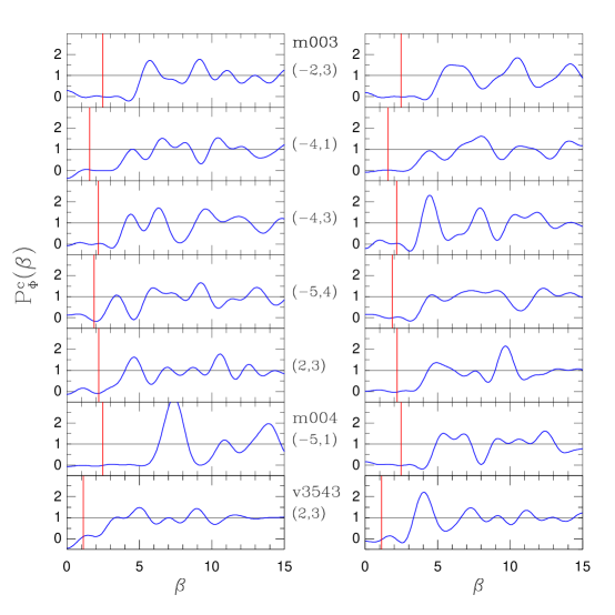
Figure 2: The primordial power spectrum ${P}^{c}_{\Phi}(\beta)$ exhibits suppression of long-wave power if the Universe has compact topology. ${P}^{c}_{\Phi}(\beta)=1$ corresponds to an infinite open Universe. Examples of the spectrum cutoff in several CH Universes are shown. The first 6 have about the same value of $R_{>}/d_{c}$, where $R_{>}$ is the minimal radius of the sphere which completely encompasses the Dirichlet domain. These spaces have volumes $V/d_{c}^{3}$ around unity. The sixth space is m004(-5,1), and the seventh one is the v3543(2,3) space with volume $V_{\!\cal M}/d_{c}^{3}=6.45$, which are used as examples of “small” and “large” spaces in this paper. The plots show the integrand for the correlation function $\xi^{c}_{\Phi}({\bf x},{\bf x}^{\prime})$ at zero separation, ${\bf x}={\bf x^{\prime}}$, at two different locations (left and right panels). This contrasts with isotropic spaces for which the integrands will be the same. The vertical line at $k=2/R_{>}$ marks the value below which there is strong suppression of large-scale power .

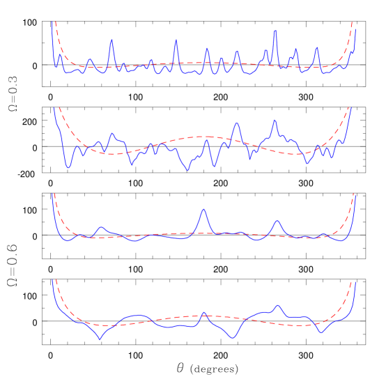
Figure 3: This shows the behavior of the correlation function of the CMB temperature on a great circle in the sky in a CH model (m004(-5,1)). The solid curves in the first and third panels show $C(\theta)$ for the surface term in the Sachs-Wolfe (NSW) effect for $\Omega_{0}=0.3$ & $0.6$, respectively. They reflect the spatial correlation along a circle on the sphere of last scattering (SLS). The number of peaks in $C(\theta)$ matches the number of Dirichlet domains that the circle intersects. The dashed curves show corresponding results for the simply connected infinite ${\cal H}^{3}$ models with $\Omega_{0}=0.3$ & $0.6$. The second and fourth panels are analogous to the first and third panels, where the integrated Sachs-Wolfe (ISW) effect is included. In this more physically correct case the sharp NSW peaks have been diluted by the ISW contributions. However, ISW induces new features, in particular, note the appearance of strong negative correlations in panels two and four.

Figure 4: This shows two full-sky CMB anisotropy maps, plotted as pairs of $180^{\circ}$ diameter hemispherical caps, one centered on the South Galactic Pole (SGP) and one on the North (NGP). They are one of an infinite number of possible random realizations based on computed pixel-pixel correlation matrix for the model in question. Both surface and integrated Sachs-Wolfe effects have been included. The power was normalized to best match the cobe data. In contrast to Figs. 5 and 6 the maps are not optimally filtered. The model labels $L(arge)CH$ and $S(mall)CH$ refer to the CH models v3543(2,3) and m004(-5,1), respectively. (The model number associated with the topology corresponds to that of the census of CH spaces from the Geometry center, Univ. of Minnesota; $SCH$ is one of the smallest and $LCH$ is one of the largest spaces in the census). The value of $\Omega_{0}$ in each was chosen so that $V_{\!\cal M}\sim V_{\sc sls}$. The matched pairs of circles expected if the CMB anisotropy is dominated by the surface terms [30] are superimposed on the map for each model. Each pair is labeled by the same number centered on the circles (and the same colour). The relative phase is shown by identified points marked by a diamond and a triangle on each circle in a pair. For clarity, we show only the eight largest pairs out of $35$ for the $LCH_{\Omega_{0}=0.6}$ case. Even at cobe–dmr resolution, we find the cross-correlation between the temperature along matched circles is very good in the $SCH_{\Omega_{0}=0.9}$ model. The ISW contribution is larger at $\Omega_{0}=0.6$, and the cross-correlation coefficients are systematically smaller for $LCH_{\Omega_{0}=0.6}$ circle pairs. The contours are linearly spaced at $30~{}\mu{\rm K}$ steps.

4.2 CMB anisotropy correlation function

In standard cosmological models based on a topologically trivial space, such as ${\cal H}^{3}$, the observed CMB photons have propagated along radial geodesics from a $2$-sphere of radius $R_{\sc ls}$ (that we refer to as the sphere of last scattering, SLS) centered on the observer. The same picture also applies to CH models when the space is viewed as a tessellation of the universal cover. If the compact space fits well within the SLS, the photons propagate through a lattice of identical domains. As a consequence, strong correlations build up between CMB temperature fluctuations observed in widely separated directions. The correlation function $C(\hat{q},\hat{q}^{\prime})$ is anisotropic and contains characteristic patterns determined by the photon geodesic structure of the compact manifold. These correlations persist even in CH models whose Dirchlet domains are comparable to or slightly bigger than the SLS. This is the key difference from the standard models where $C(\hat{q},\hat{q}^{\prime})$ depends only on the angle between $\hat{q}$ and $\hat{q}^{\prime}$ and generally falls off with angular separation.

In Figure 3, the complex behavior of the correlation function is illustrated with the example of the small CH model (m004(-5,1)). The SLS encompasses $\approx 150$ domains for $\Omega_{0}=0.3$ and $\approx 20$ domains for $\Omega_{0}=0.6$ and is comparable to the size of one domain for $\Omega_{0}=0.9$. The angular correlation along any arbitrary great circle in the sky in lower $\Omega_{0}$ models shows distinct peaks as one encounters repeated copies of the Dirichlet domain. The peaks are more pronounced when one considers only the surface terms of eq.(2) in the CMB anisotropy. Including the line of sight ISW contribution tends to smear the peaks but adds its own characteristic features [9].

Consider compact universe models which are small enough such that the SLS does not completely fit inside one domain, $R_{\sc ls}>R_{<}$. The CMB temperature is expected to be identical along pairs of circles if temperature fluctuations are dominated by the surface terms at the SLS [30]. We identify these matched circles on the sky in our models and check the extent of cross correlation seen at the angular resolution of cobe–dmr. Figure 4 show the matched pairs of circles in two (“small” and “large”) CH models superimposed on random realizations of the theoretical sky generated from the computed pixel-pixel correlation matrix for these models. The models were chosen to have a volume comparable to the volume $V_{\sc sls}$ within the SLS. Even with the coarse pixelization of cobe–dmr, we do see fairly good cross-correlation in the CMB temperature along matched circles in our realizations. Again, the pattern of correlated circles is more pronounced when the surface terms are dominant, as happens in the small model ($SCH$) with $\Omega_{0}=0.9$. The cross-correlation coefficient $\rho$ between the circles is in the range $\rho\approx 0.6-0.95$ in this case, whereas it is in the range $\rho\approx 0.2-0.6$ for the large model ($LCH$) with $\Omega_{0}=0.6$.

The circles of identified pixels on the SLS are not the whole story [9]. Enhanced NSW cross-correlations, but at a lower level, also exist between all pairs of points on the SLS which are projected close to each other on the CH manifold. This can be seen as secondary maxima in the examples in Figure 3; these are absent in standard cosmological models. Some features persist at a detectable level even when the compact universe encompasses the SLS, i.e., $R_{\sc ls}\mathrel{\hbox to0.0pt{\lower 3.0pt\hbox{$\mathchar 536\relax$}\hss}\raise 2.0pt\hbox{$\mathchar 316\relax$}}R_{<}$ , although circles are absent in this case (the effect dies out for $R_{\sc ls}\ll R_{<}$). When the relative ISW component is significant, the geometrical patterns based on pointwise identifications on the SLS are supplanted by more complex features arising from identifications between photon geodesics, e.g., the strong negative correlations evident in Figure 3. Correlation features also arise from the global inhomogeneity of CH spaces since it implies that the rms temperature fluctuations varies with location in the sky in a pattern set by the topology of the space.

The reader’s intuition can be sharpened with examples from simpler topologies. Flat torus models exhibit forward-backward correlation symmetry along their axes [12, 14]. Patterns in CMB temperature maps have also been discussed for other flat models in  [15]. An example of a hyperbolic model is the non-compact horn-like space [16] for which  [15] argue the CMB sky will exhibit a flat spot.

4.3 Bayesian analysis constraints from cobe–dmr

As discussed above, compact models which are not much larger than the sphere of last scattering tend to show significant correlated patterns in the CMB sky. To the extent that these correlations are absent in the cobe–dmr data, the models tend to be at odds with observations. Figures 5 and 6 compare theoretical realizations of the CMB anisotropy in the $LCH$ and $SCH$ models with the cobe–dmr data. They should be compared with the ‘DATA’ map in Fig. 5, a Wiener filtered picture of the CMB data, using a theoretical model which best-fits the data. What one should be noting is the shapes of the patterns and not the specific locations of the patterns, since these can change from realization to realization. The full Bayesian analysis takes into account all possible realizations. The incompatibility of models with small $V_{\cal M}/V_{\sc sls}$ (SCH-$\Omega_{0}=0.3,0.6$) is visually obvious: the best fit amplitudes are high which is reflected in the steeper hot and cold features. Although, SCH-$\Omega_{0}=0.9$ and LCH-$\Omega_{0}=0.6$ do not appear grossly inconsistent, the intrinsic anisotropic correlation pattern is at odds with the data statistically.

Figure 5: The figure consists of a column of three CMB sky-maps showing a pair of $140^{\circ}$ diameter hemispherical caps each, centered on the South (SGP) and North (NGP) Galactic Poles, respectively. The top map labeled DATA, shows the cobe–dmr 53+90+31 GHz A+B data after Wiener filtering assuming a standard CDM model, normalized to cobe. The next two maps are one random realization of the CMB anisotropy in v3543(2,3) – our choice of a $L(arge)CH$ model example, for $\Omega_{0}=0.6~{}\&~{}0.8$ based on our theoretical calculations of $C(\hat{q},\hat{q}^{\prime})$ convolved with the cobe–dmr beam. Both surface and integrated (ISW) Sachs-Wolfe effects have been included in $C(\hat{q},\hat{q}^{\prime})$. No noise was added. The power was normalized to best match the cobe data. The theoretical sky was optimally filtered using the cobe experimental noise to facilitate comparison with data. LCH with $\Omega_{0}=0.8$ is compatible with the data with a suitable choice of orientation while $\Omega_{0}=0.6$ is ruled out (See Table LABEL:tab:logprob). For all the maps in Figs. 5 and 6, the average, dipole and quadrupole of the $|b|>20^{\circ}$ sky were removed and a $20^{\circ}$ Galactic latitude cut was used, with extra cuts to remove known regions of Galactic emission proposed by the cobe team accounting for the ragged edges. The contours are linearly spaced at $15~{}\mu{\rm K}$ ($\Delta T/T=0.55\cdot 10^{-5}$) steps. The maps have been smoothed by a $1.66^{\circ}$ Gaussian filter.

Figure 6: The three CMB sky-maps showing a pair of $140^{\circ}$ diameter hemispherical caps each, centered on the South (SGP) and North (NGP) Galactic Poles, are analogous to the lower two plots in Fig. 5 but for the $S(mall)CH$ model m004(-5,1). The fact that $\Omega_{0}=0.3~{}\&~{}0.6$ models above are strongly ruled out by the cobe data is obvious visually, while the $\Omega_{0}=0.9$ can be excluded on the basis of our Bayesian analysis. (See Table LABEL:tab:logprob.)

On each of our selection of models, we have carried out a fully Bayesian analysis of the probability of the model given the cobe–dmr 4yr data. In Table LABEL:tab:logprob, we present the relative likelihood of the selected models to that of the infinite ${\cal H}^{3}$ model with the same $\Omega_{0}$.

Table 1: The Log-likelihoods of the compact hyperbolic models relative to the infinite models with same $\Omega_{0}$ are listed. The probabilities are calculated by confronting the models with cobe–dmr data. The values quoted are likelihoods marginalized over the amplitude of the initial power spectrum. The volume within the sphere of last scattering (SLS) relative to the volume of the compact models of the universe ($V_{\rm SLS}/V_{\!\cal M}$) is listed. The three columns of logarithm of likelihood ratios ${\cal L}/{\cal L}_{0}$ correspond to the best, next best and the worst values that we have obtained amongst $24$ different rotations of the compact space relative to the sky. The number $\nu$ in brackets gives the conventional, albeit crude, translation of the probabilities to a Gaussian likelihood ${\cal L}/{\cal L}_{0}\sim\exp[-\nu^{2}/2]$. Only the last model in a specific orientation appears to be consistent with the cobe–dmr data.

• CH Topology	$\Omega_{0}$	$V_{\rm SLS}/V_{\!\cal M}$	Log of Likelihood Ratio (Gaussian approx.)
  $[{\cal V}_{\!\cal M},R_{>}/d_{c}]$			Orientation
  			‘best’	‘second best’	‘worst’
  	0.3	153.4	-35.5 (8.4$\sigma$)	-35.7 (8.4$\sigma$)	-57.9 (10.8$\sigma$)
  m004(-5,1)	0.6	19.3	-22.9 (6.8$\sigma$)	-23.3 (6.8$\sigma$)	-49.4 ( 9.9$\sigma$)
  $[0.98,0.75]$	0.9	1.2	-4.4 (3.0$\sigma$)	-8.5 (4.1$\sigma$)	-37.4 ( 8.6$\sigma$)
  v3543(2,3)	0.6	2.9	-3.6 (2.7$\sigma$)	-5.6 (3.3$\sigma$)	-31.0 (7.9$\sigma$)
  $[6.45,1.33]$	0.8	0.6	2.5 (2.2$\sigma$)	-0.8 (1.3$\sigma$)	-12.6 (5.0$\sigma$)

(The cobe data alone does not strongly differentiate between the infinite hyperbolic models with different $\Omega_{0}$.) The anisotropy of the theoretical $C(\hat{q},\hat{q}^{\prime})$ causes the likelihood of compact models to vary significantly with the orientation of the space with respect to the sky, depending on how closely the features in the single data map available to humans match (or mismatch) the pattern predicted in $C(\hat{q},\hat{q}^{\prime})$. Some optimal orientations may also have the “ugly” correlation features hidden in the Galactic cut. We analyzed $24$ different orientations for each of our models and found that only the model with $V_{\cal M}>V_{\sc sls}$ (LCH-$\Omega_{0}=0.8$) cannot be excluded. (At one orientation this model is even preferable to standard CDM; this raises a question of the statistical significance of any detection of intrinsic anisotropy of a space when only a single realization of data is available.)

Similar conclusions were reached by some of the authors (JRB, DP and I. Sokolov [14]) for flat toroidal models. Comparison of the full angular correlation (computed using the eigenfunction expansion, eq.(4)) with the cobe–dmr data led to a much stronger limit on the compactness of the universe than limits from other methods [12, 13]. The main result of the analysis was that $V_{\sc sls}/V_{\!\cal M}<0.4$ at $95\%~{}CL$ for the equal-sided $3$-torus. For $3$-tori with only one short dimension (or for the non-compact $1$-torus), the constraint on the most compact dimension is not quite as strong because the features can be hidden in the “zone of avoidance” associated with the Galactic cut.

Although our results strongly indicate that manifolds with small $V_{\!\cal M}/V_{\sc sls}$ are unlikely to survive confrontation with the cobe–dmr data, we emphasize that when this ratio becomes of order unity very interesting correlation patterns appear which, for certain orientations, may even be preferred by the cobe–dmr data. Since manifolds with large $V_{\!\cal M}/d_{c}^{3}$ allow low values of $\Omega_{0}$ while still avoiding small $V_{\!\cal M}/V_{\sc sls}$, even large mean curvatures may be compatible, and certainly the $\Omega_{0}\sim 0.3-0.6$ values that some of the astrophysical data currently prefers can still be nicely accommodated within the CH framework. Of course, there are many more manifolds for which $R_{<}$ may be small but $R_{>}$ large, for whom the constraints will be even more dependent upon how specific orientations may deliver unwanted correlation features into the zone of avoidance, as the asymmetric 3-torus results reveal, or line up predicted correlation patterns with chance upward or downward fluctuations in the data. When $R_{<}$ is large compared to $R_{\sc ls}$, we expect the results will quickly converge towards the usual infinite hyperbolic manifold results. The intermediate terrain still encompasses ample scope for interesting topological signatures to be discovered within the CMB. Although our methods are quite general, testing all manifolds in the SnapPea census this way is rather daunting, and there are countably infinite manifolds not yet prescribed. What may be more promising for discovery are specialized statistical indicators, which are less sensitive than the full Bayesian approach we have used here, but not as manifold sensitive; e.g., the statistical techniques which exploit the high degree of correlations along circle pairs that [30] have emphasized, and Fig. 4 reveals. Maps like we have constructed will be necessary to test the statistical significance of such methods. We also note that dramatically increasing the resolution beyond that of cobe–dmr is quite feasible with current computing power using our techniques.

5 Acknowledgements

We thank Jeff Cheeger for illuminating discussions. We also thank the Geometry center of the University of Minnesota for making a lot of useful material available on their website, in particular, the SnapPea package. We thank the anonymous referee for pointing out related literature [7, 20].

References

References

- [1] Dekel A, Burstein D and White S D M 1996 in Critical Dialogues in Cosmology, ed. Turok N (Singapore: World Scientific); Spergel D N, in this volume.
- [2] Ellis G F R 1971 Gen. Rel. Grav. 2 7 ; Lachieze-Rey M and Luminet J-P 1995, Phys. Rep. 25 136; Cornish N J, Spergel D N and Starkman G D 1996, Phys. Rev. Lett. 77, 215.
- [3] Weeks J R SnapPea: A computer program for creating and studying hyperbolic 3-manifolds University of Minnesota Geometry Center.
- [4] Thurston W P 1979 The Geometry of 3-Manifolds, lecture notes, Princeton University; Thurston W P & Weeks J R 1984 Sci. Am. (July) 108.
- [5] Weeks J R 1985 Ph.D. Thesis, (Princeton); Matveev S V and Fomenko A T 1988 Usp. Mat. Nauk. 43 5 [Russ. Math. Surv. 43 3 (1988)].
- [6] Gabai D, Meyerhoff R G and Thurston N preprint MSRI 1996-058
- [7] Culler M and Shalen P B 1992 J. Amer. Math. Soc. 5 231; ibid 1997 Proc. Amer. Math. Soc. 125 3059; ibid 1994 Proc. Amer. Math. Soc. 120 1281; ibid 1994 Invent. Math. 118 285; Culler M Hersonsky S and Shalen P B 1998 Topology 37 805; Anderson J W, Canary R D, Culler M and Shalen P B 1996 J. Diff. Geom. 43 738.
- [8] Mukhanov V F, Feldman H A and Brandenberger R H 1992 Phys. Rep. 215 203.
- [9] Bond J R, Pogosyan D and Souradeep T preprint.
- [10] Bond J R 1996 Theory and Observations of the Cosmic Background Radiation, in “Cosmology and Large Scale Structure”, Les Houches Session LX, August 1993, ed. R. Schaeffer, Elsevier Science Press.
- [11] Bond J R, Pogosyan D and Souradeep T 1997 in: Proceedings of the XVIIIth Texas Symposium on Relativistic Astrophysics,ed. Olinto A, Frieman J and Schramm D N, (World Scientific).
- [12] Starobinsky A A 1993 JETP Lett. 57 622; de Oliveira Costa A, Smoot G F and Starobinsky A A 1996 Ap. J. 468 457.
- [13] Sokolov I Y 1993 JETP Lett. 57 617; Stevens D, Scott D and Silk J 1993 Phys. Rev. Lett. 71 20; de Oliveira Costa A & Smoot G F 1995 Ap. J. 448 477.
- [14] Bond J R 1997 Proc. of the XVIth Moriond Astrophysics Meeting, ed. Bouchet F R et al. ., (Paris: Editions Frontieres); Bond J R 1998 Proc. Natl. Acad. Sci. USA 95 35.
- [15] Levin J J, Barrow J D, Bunn E F and Silk J 1997 Phys. Rev. Lett. 79 974; Levin J J, Scannapieco E and Silk J, in this volume.
- [16] Sokoloff D D and Starobinski A A 1975 Sov. Astron. 19 629.
- [17] Harrison E 1967 Rev. Mod. Phys. 39 862.
- [18] Lyth D H and Stewart E D 1990 Phys. Lett. B252 336.
- [19] Ratra B and Peebles P J E 1994 Ap. J. Lett.432 L5.
- [20] Aurich R and Steiner F 1992 Proc. R. Soc. Lond. A437 693.
- [21] Chavel I 1984 Eigenvalues in Riemannian geometry (New-York: Academic Press).
- [22] Hardy G H 1956 Divergent Series (London: Oxford University Press).
- [23] Bennett C et al. 1996 Ap. J. Lett.464 L1; and 4-year DMR references therein.
- [24] Bond J R 1994 Phys. Rev. Lett. 74 4369.
- [25] Balazs N L and Voros A 1986 Phys. Rep. 143 109.
- [26] Cheeger J 1970 Problems in Analysis (A Symposium in honor of S. Bochner) (Princeton: Princeton University Press).
- [27] Buser P 1980 Proc. Symp. Pure Math. 36 29.
- [28] Berard P H 1980 Spectral Geometry: Direct and Inverse Problems, Lec. Notes in mathematics, 1207 (Berlin: Springer-Verlag).
- [29] Buser P 1982 Ann. scient. Ec. Norm. Sup. 15 213.
- [30] Cornish N J, Spergel D N and Starkman G D 1996 preprint gr-qc/9602039; ibid., in this volume.