(a)                                                            (b)

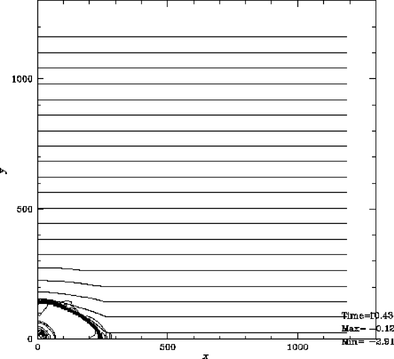
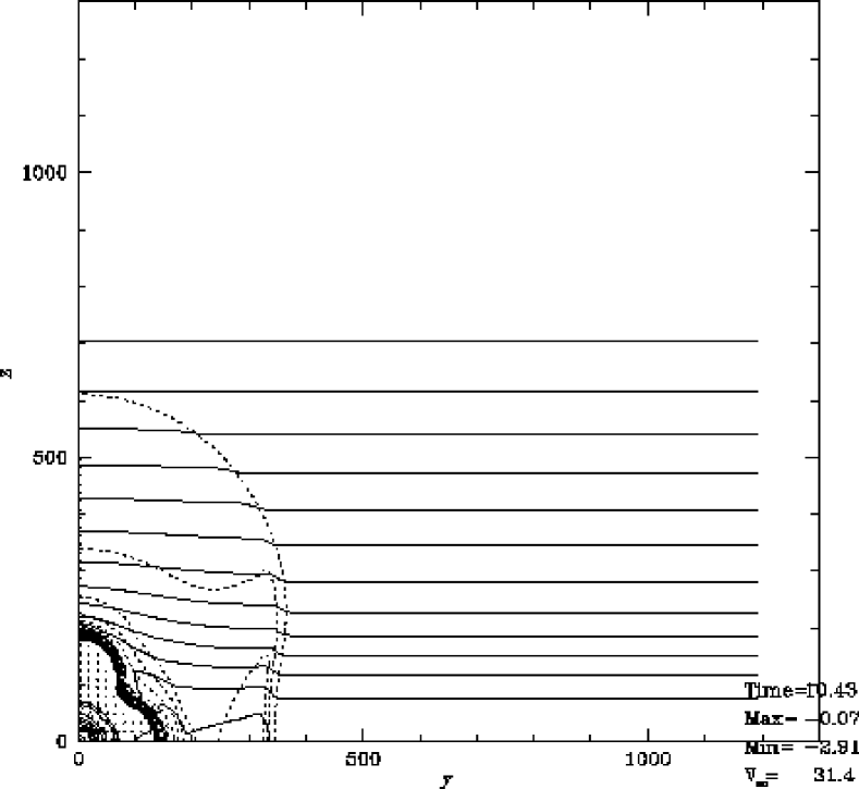
(c)

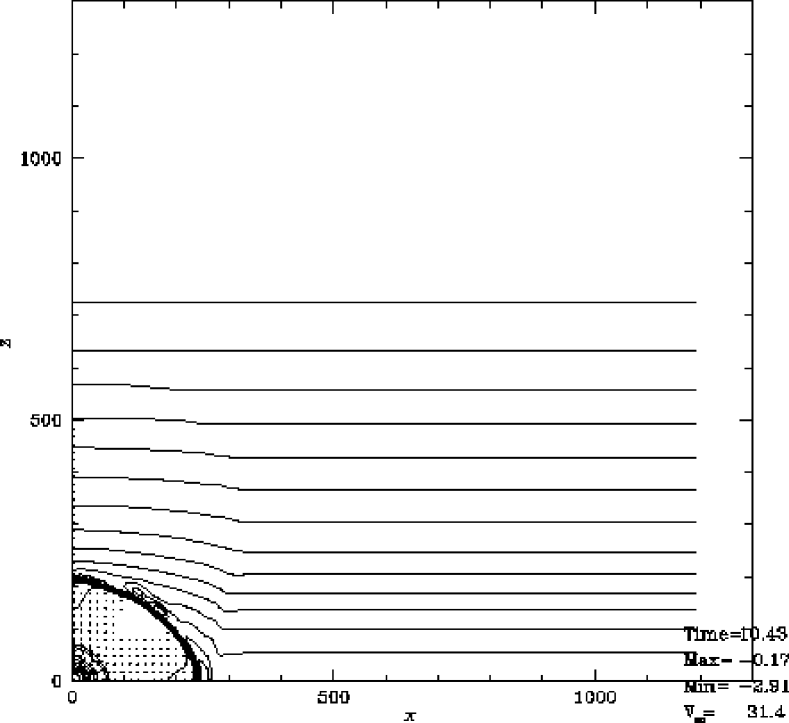
Figure 1: (a): A cross-cut along the mid-plane of the disk, $z=0$, at $t=10.4$ Myr. Density contour lines and magnetic field lines (running horizontally) are plotted. The numbers near the bottom-right corner represent, respectively, the time of the snapshot, the maximum and minimum levels of the contours, e.g., 21 contour lines are plotted for the values from $10^{-3.10}\rm cm^{-3}$ to $10^{-0.38}\rm cm^{-3}$. (b): The same as (a) but for the $x=0$ plane. Density contour lines and velocity fields are plotted. The magnetic field is running perpendicular to this plane and its distribution is represented by dotted contour lines. The maximum speed plotted in the panel is also shown near the bottom-right corner. (c): The same as (b) but for the $y=0$ plane.

(a)                                                            (b)

(c)

Figure 2: Physical quantities are plotted along the $x-$ (a), $y-$ (b), and $z-$axis (c). The density $n{\rm(cm^{-3})}$ (solid lines), the temperature $T{\rm(10^{4}K)}$ (dotted lines), the magnetic flux density $B_{x}{\rm(\mu G)}$ (dashed lines), and the velocities along the respective axes $|v|{\rm(km~{}s^{-1}})$ (long-dashed lines) are plotted. This is a snapshot at the age of $t=10.4$ Myr.

(a)                                                            (b)

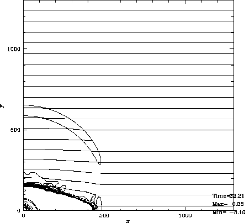
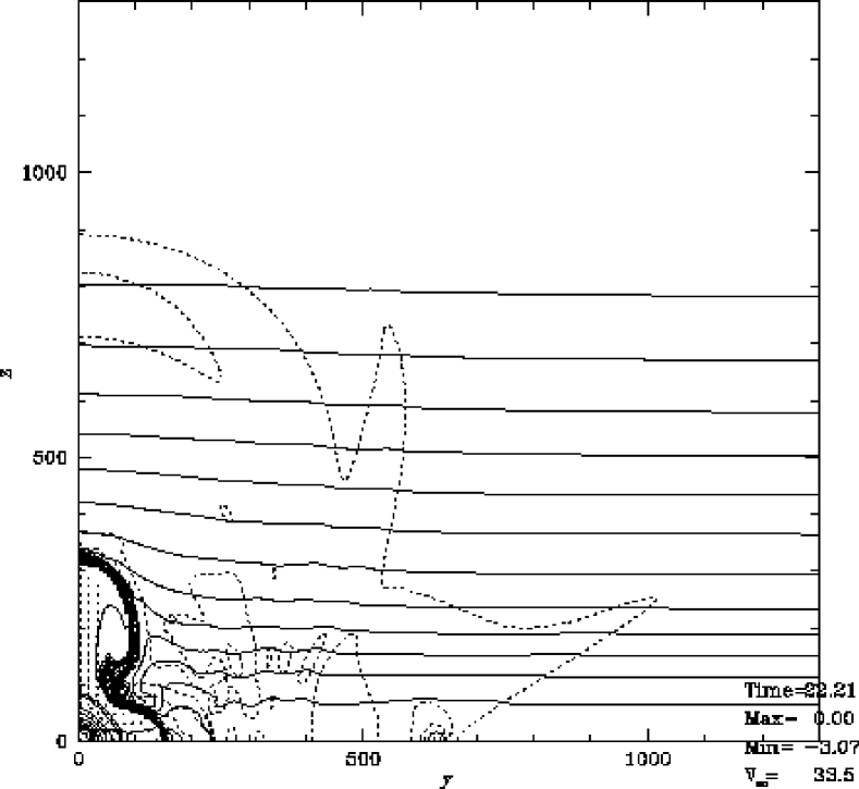
(c)

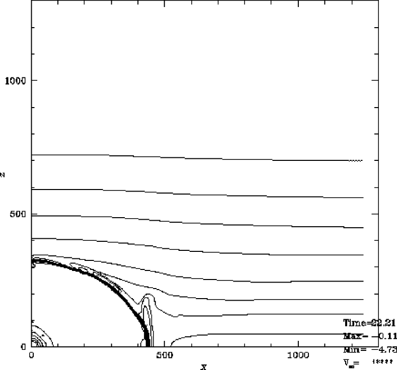
Figure 3: The same as Fig.1, but for the age of $t=22$ Myr.

(a)                                                            (b)

(c)

Figure 4: The same as Fig.2, but for the age of $t=22$ Myr.

(a)                                                            (b)

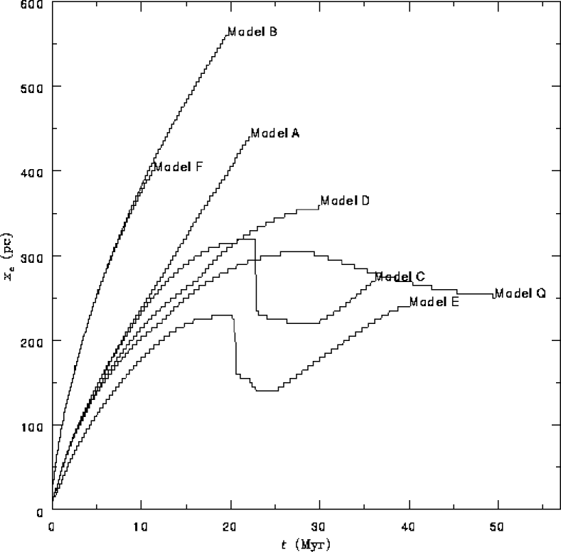
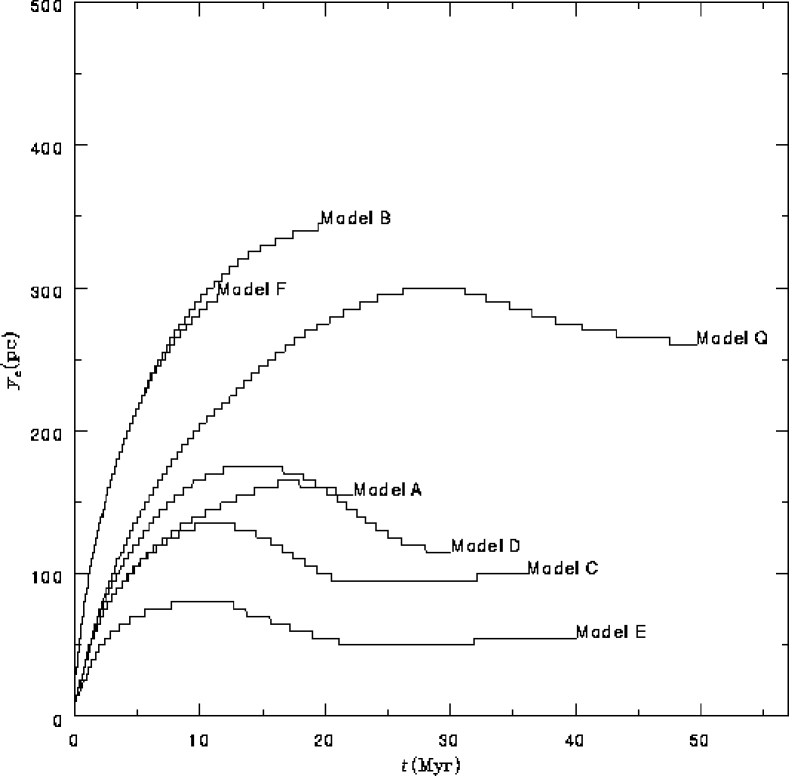
(c)

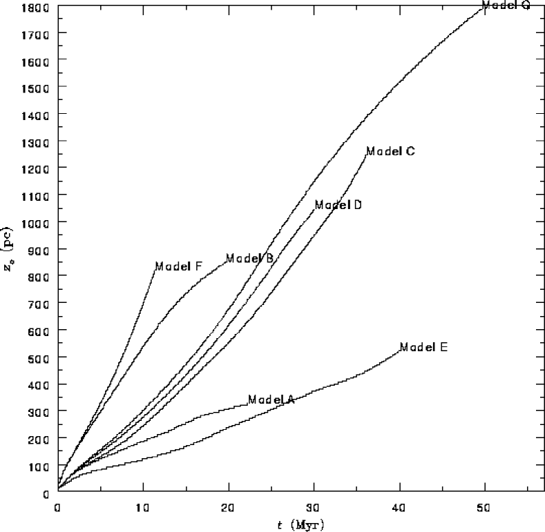
Figure 5: Expansion law of a hot cavity formed in a superbubble. The size of the hot cavity is measured with ($x_{c},y_{c},z_{c}$). Models A and B correspond to the cases that a superbubble is formed in ISM with a uniform magnetic field distribution. In Models C, D, E, and F, the magnetic field strength was assumed to decrease upwardly, while the Alfven speed $B/(4\pi\rho)^{1/2}$ is constant. Model Q, non-magnetic superbubble, is also plotted.

(a)                                                            (b)

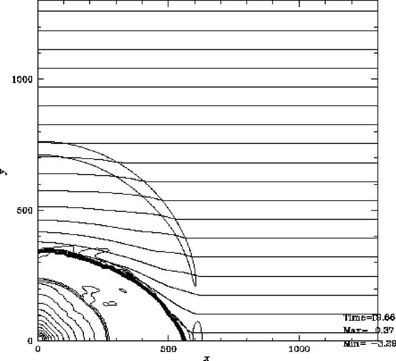
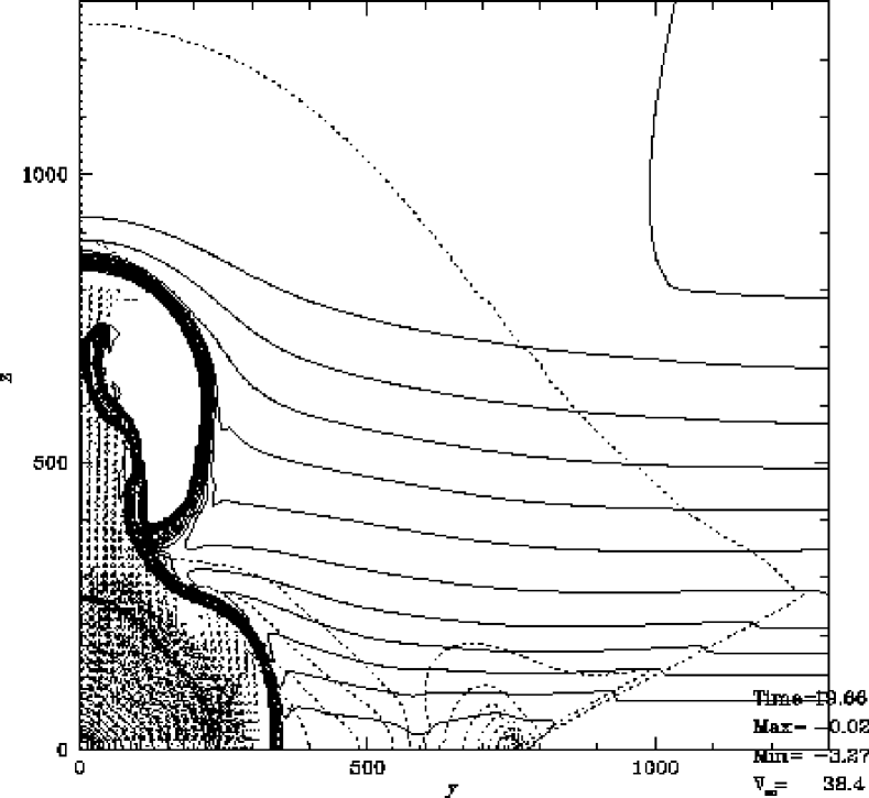
(c)

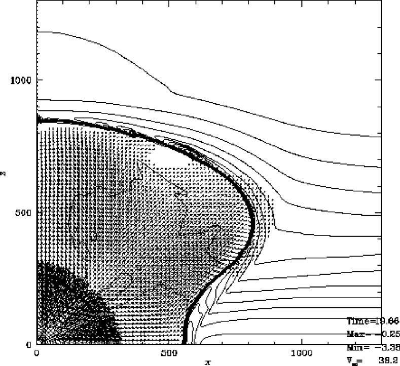
Figure 6: A superbubble driven by an active OB association with a luminosity 10 times larger than the previous model. This is a snapshot at the age of $t=20$ Myr.

(a)                                                            (b)

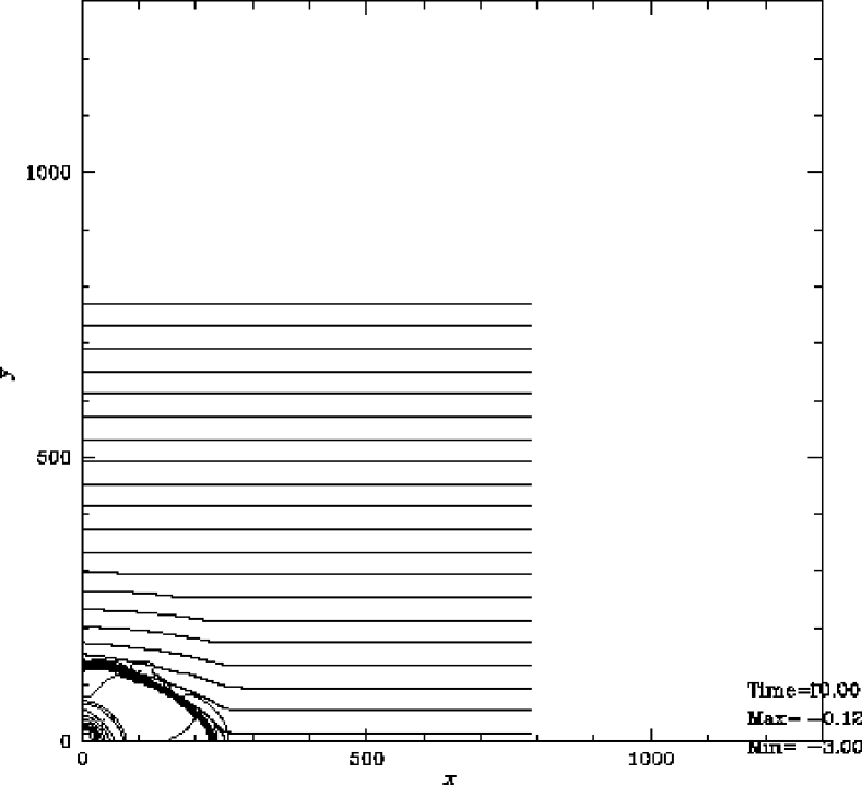
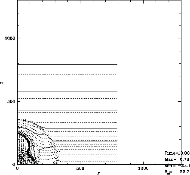
(c)

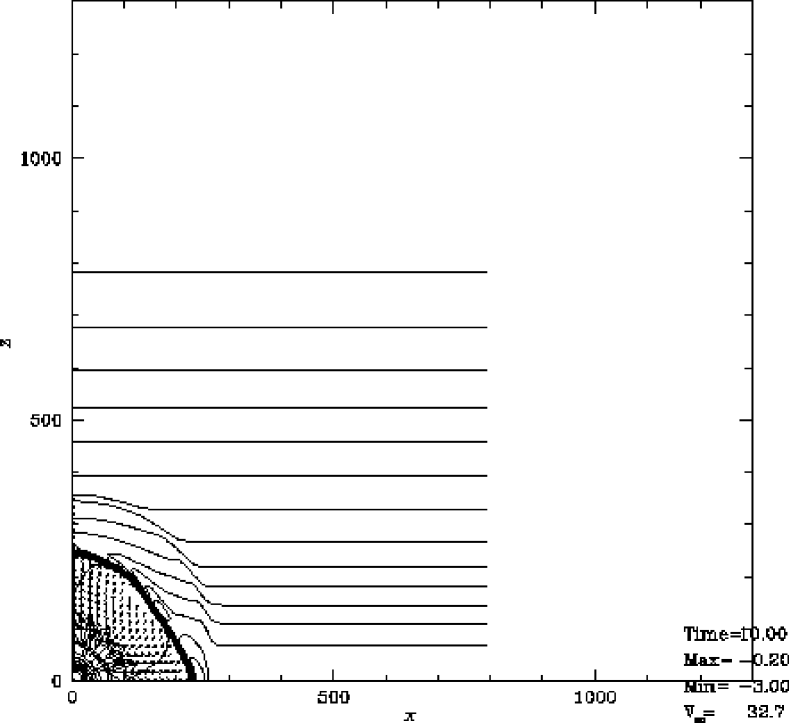
Figure 7: The same as Fig.1 but for the model of $B_{0}\propto\rho^{1/2}$. Panels (a), (b) and (c) are the snapshots of $t=10$ Myr. Panels (d), (e) and (f) are those of $t=22.8$ Myr and (g), (h) and (i) are for $t=30$ Myr.

(a)                                                            (b)

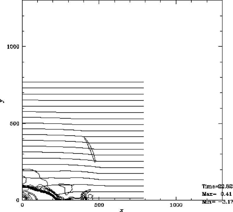
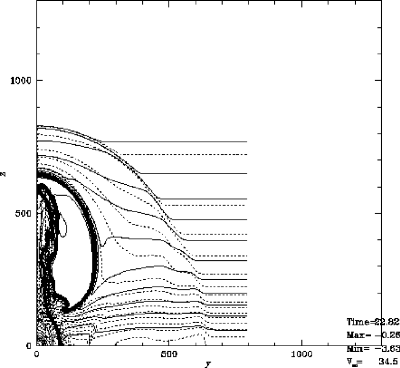
(c)

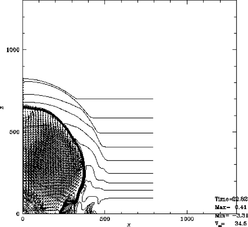
Figure 7: continued.

(a)                                                            (b)

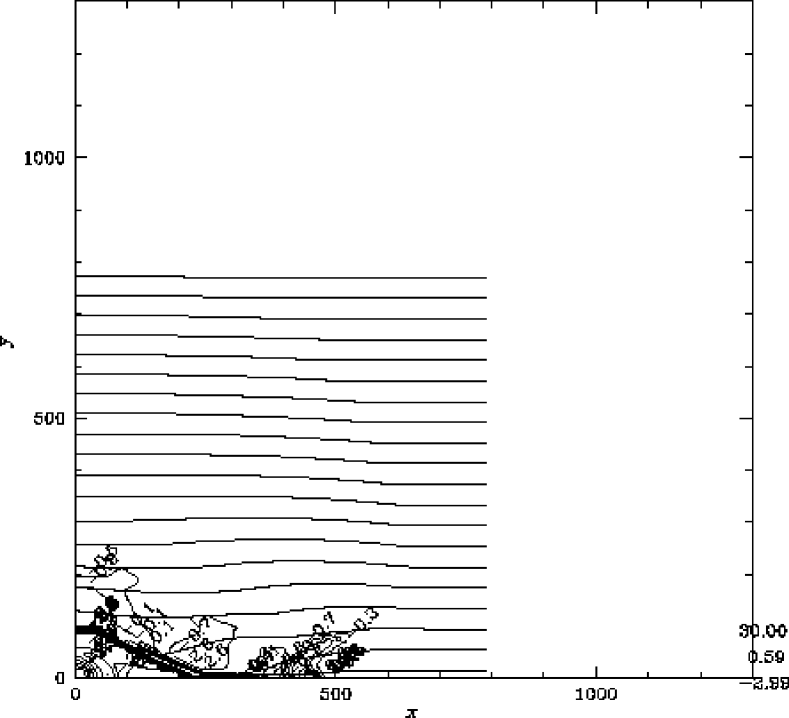
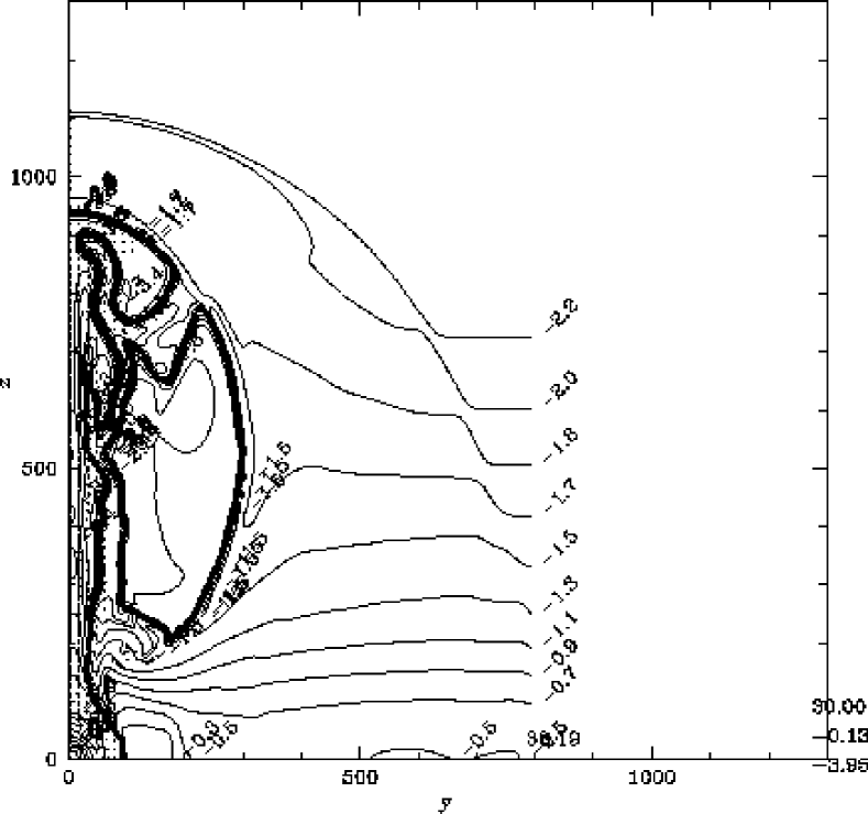
(c)

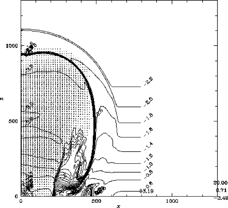
Figure 7: continued.

(a)                                                            (b)

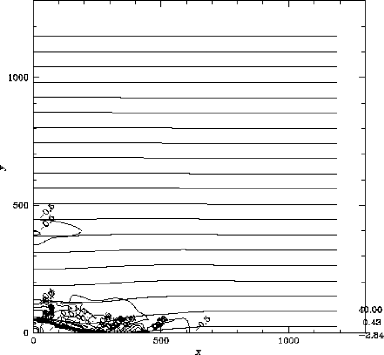
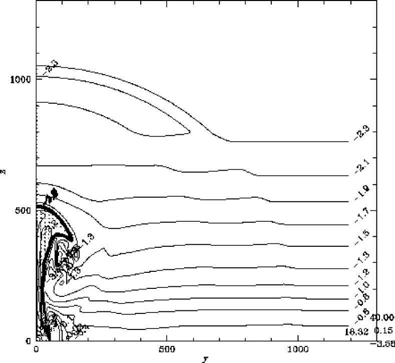
(c)

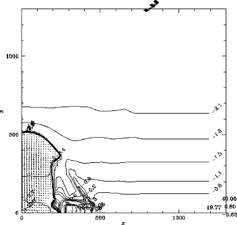
Figure 8: The same as Fig.7 but for a model with a less mechanical luminosity of $L_{\rm SN}=10^{37}{\rm erg/s}$. The snapshot corresponds to $t=40$ Myr.

Figure 9: Expansion law for a thin-shell model. External interstellar pressures are chosen equal to $p_{\rm out}=1.7\times 10^{-12}{\rm erg~{}cm^{-3}}$ (solid line), $p_{\rm out}=1\times 10^{-12}{\rm erg~{}cm^{-3}}$ (dotted line), and $p_{\rm out}=0$ (dashed line). The Weaver et al.’s (1977) solution is similar to a dashed curve and the point when the ram pressure is equal to the interstellar pressure with $p_{\rm out}=1.7\times 10^{-12}{\rm erg~{}cm^{-3}}$ is also plotted by a asterisk. The equivalent radii which are defined as $r_{\rm equiv}=(3V_{\rm hot}/4\pi)^{1/3}$ for Models A and C are also illustrated with dash-dotted lines (lower:A; upper:C).