ESO Imaging Survey

Abstract

Preliminary results of a search for distant clusters of galaxies using the recently released I-band data obtained by the ESO Imaging Survey are presented. In this first installment of the survey, data covering about 3 square degrees in I-band are being used. The matched filter algorithm is applied to two sets of frames that cover the whole patch contiguously and these independent realizations are used to assess the performance of the algorithm and to establish, from the data itself, a robust detection threshold. A preliminary catalog of distant clusters is presented, containing 39 cluster candidates with estimated redshifts $0.3\leq z\leq 1.3$ over an area of 2.5 square degrees.

1 Introduction

One of the primary goals for undertaking the ESO Imaging Survey (EIS; Renzini & da Costa 1997) has been the preparation of a sample of optically-selected clusters of galaxies over an extended redshift baseline for follow-up observations with the VLT. High-redshift clusters are, of course, a primary target for 8-m class telescopes. A large and well defined sample of clusters can be used for many different studies, ranging from the evolution of the galaxy population, to the search for arcs and lensed high redshift galaxies, to the evolution of the abundance of galaxy clusters, a powerful discriminant of cosmological models. In addition, individual clusters may be used for weak lensing studies and as natural candidates for follow-up observations at X-ray and mm wavelengths, which would provide complementary information about the mass of the systems. For some of these applications it suffices to find a large number of clusters, while for others it is vital to obtain a full understanding of the selection effects, to generate suitable statistical samples.

Until recently, only a handful of clusters were known at redshifts $z\leavevmode\nobreak\ \hbox to0.0pt{$>$\hss}{\lower 4.30554pt\hbox{$\sim$}}0.5$; visual searches for high redshift clusters were conducted by Gunn et al. (1986) and Couch et al. (1991), but their samples are severely incomplete beyond $z\sim 0.5$; at higher redshifts targeted observations in fields containing known radio-galaxies and QSOs have produced a handful of cluster identifications (e.g., Dickinson 1995; Francis et al. 1996; Pascarelle et al. 1996; Deltorn et al. 1997). The first objective search for distant clusters was conducted by Postman et al. (1996; hereafter P96) using the 4-Shooter camera at the 5-m telescope of the Palomar Observatory. In their survey 10 out of the 79 cluster candidates have estimated redshift $\leavevmode\nobreak\ \hbox to0.0pt{$>$\hss}{\lower 4.30554pt\hbox{$\sim$}}0.7$. Further evidence for the existence of clusters at high redshift has been obtained from X-ray (e.g., Gioia & Luppino 1994; Henry et al. 1997; Rosati et al. 1998), optical (e.g., Connolly et al. 1996; Zaritsky et al. 1997) and infrared (Stanford et al. 1997) searches. However, the existing samples are small, and their selection effects largely unknown.

Recently, observations of the first patch of the EIS, covering about 3 square degrees, have been completed, and the data made available to the community (Nonino et al. 1998; hereafter Paper I). Although the data are still in a preliminary form, much can already be learned regarding the characteristics of the sample of candidate clusters that can be detected using the EIS data. In this paper preliminary catalogs of objects detected on single 150 sec. I band frames are used (see Sects. 2 and 3) mainly to assess the capability of the EIS to detect clusters of galaxies at $z\leavevmode\nobreak\ \hbox to0.0pt{$>$\hss}{\lower 4.30554pt\hbox{$\sim$}}0.5$. A discussion of a full cluster sample based on the galaxy catalog extracted from the coadded EIS images, is postponed to a future paper (Scodeggio et al. 1998). The reason for using here the single-frame catalogs is that they provide two independent datasets for the same area of the sky. The comparison between the cluster detections obtained using the two catalogs separately, can be used to quantify the reliability of the cluster detection procedure. When the handling of catalogs extracted from the coadded images is fully implemented in the EIS data reduction pipeline, the cluster search will be carried out using those catalogs, instead of the single-frame ones, to benefit from the deeper limiting magnitude of the coadded images.

In the meanwhile a better quantification of the detection limits for distant clusters of galaxies within the EIS data could be obtained by comparing the results presented here with those obtained using independent cluster search methods.

In Sects.  2 and  3 the observations, data reduction and the object catalogs, that are used for the cluster search, are briefly discussed. The cluster finding procedure, based on the matched-filter algorithm proposed by P96, is described in Sect. 4. In Sect.  5 the preliminary cluster catalog is presented, and the properties of the detected candidates are discussed. In Sect.  6 conclusions of this work are summarized, and its possible extensions to the search for clusters using the coadded EIS images discussed.

2 Observations and Data Reduction

The observations for the EIS are being conducted using the EMMI camera (D’Odorico 1990) on the ESO 3.5m New Technology Telescope. The effective field-of-view of the camera is about $9^{\prime}\times 8.5^{\prime}$, with a pixel size of 0.266”. Observations are being carried out over four pre-selected patches of the sky, spanning a wide range in right ascension. In this paper only the data obtained in the first of these patches, at $\alpha\sim 22^{h}45^{m}$ and $\delta$ = -40^∘ (hereafter Patch A) are used. Observations in this patch were obtained during six different runs, from July to November 1997, and cover a total area of 3.2 square degrees in I band. The I filter that is being used has a wide wavelength coverage, and the response function can be found in Paper I. The EIS magnitude system is defined to correspond to the Johnson-Cousins system, for zero-color stars.

The EIS observations consist of a sequence of 150 sec exposures. Each point of a patch is imaged twice (except at the edges of the patch), for a total integration time of 300 sec, using two frames shifted by half an EMMI-frame both in right ascension and declination. The easiest way of visualizing the global geometry of this mosaic of frames is to consider two independent sets of them, forming contiguous grids (in the following referred to as odd and even frames), superposed and shifted by half a frame both in right ascension and declination.

Observations were carried out in regular visitor mode, and observing conditions varied quite significantly from run to run, and also from night to night within a single run. This fact translates into a considerable spread in the data-quality of different EIS frames. The seeing and limiting 1$\sigma$ isophote in one arcsec² distributions for Patch A observations are shown in Fig. 1 for the odd and even frames. The median values for the combined sample are 1.10” and 23.94 mag/arcsec², respectively.

Figure 1: The data-quality as measured from the seeing and limiting isophote distributions. The top panel shows the seeing distribution for the odd (dashed line) and even (dotted line) tiles in Patch A. The median for the combined sample is 1.10”. The bottom panel shows the distribution of limiting isophotes in mag/arcsec². The median limiting isophote for the combined sample is 23.94 mag/arcsec².

The data reduction is carried out automatically through the EIS pipeline, described in Paper I. Even though the pipeline was designed to produce coadded images, it also produces fully corrected single frames, using the astrometric and photometric solution derived from the global data reduction process. The astrometric solution is found relative to the USNO-A1 catalog. The internal accuracy of the astrometric solution is better than 0.03 arcsec, although the absolute calibration suffers from the random and systematic errors of the reference catalog. It is important to emphasize, however, that the internal accuracy is more than adequate for the relative positioning of the slits in the first generation of VLT instruments such as FORS. It is also worth reminding that the pointing accuracy of the VLT is foreseen to be no better than 1 arcsec at first light. The photometric calibration is done in a two step procedure first bringing all the frames to a common photometric zero-point, taking advantage of the overlap between the frames, then an absolute calibration is made based on external data. The internal accuracy of the photometric calibration is $\leavevmode\nobreak\ \hbox to0.0pt{$<$\hss}{\lower 4.30554pt\hbox{$\sim$}}0.005$  mag. The current absolute calibration uncertainty is $\leavevmode\nobreak\ \hbox to0.0pt{$<$\hss}{\lower 4.30554pt\hbox{$\sim$}}0.2$  mag. Further details can be found in Paper I.

3 Galaxy Catalog

Even though the ultimate objective of the pipeline is to produce an object catalog extracted from the coadded image, one of its intermediate products is a multiple entry object catalog that includes all detected objects in all individual frames. This object catalog is a multi-purpose element of the pipeline, and from it several catalogs are derived. Among them are the odd and even catalogs, which are single entry catalogs listing all objects detected in the even or odd frames. To build these catalogs, multiple detections in the small overlap regions are appropriately associated to a single object, as described in Paper I.

Fig. 2 shows the projected distribution of galaxies with $I\leq 23$ from the even catalog of Patch A, for a total of 113,298 objects. The figure only shows the area with full coverage from both even and odd tiles, totaling 2.91 square degrees.

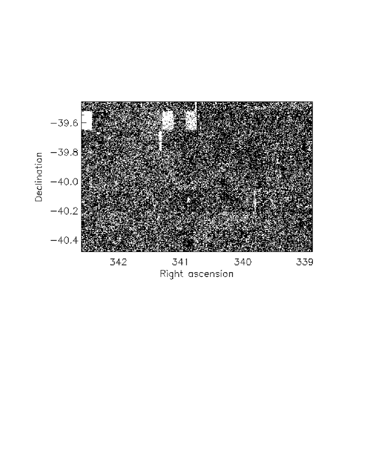
Figure 2: The projected distribution of galaxies with $I\leq 23$ included in the even I-band catalog for Patch A, limited to the region fully covered by both even and odd tiles. The marked region is the region which was excluded from the analysis because of its obvious incompleteness.

In Paper I the reliability and completeness of the single-frame catalogs were explored by comparing the deep reference field (see Paper I) with the individual frames obtained for that field. Based on that analysis, it was estimated that the single-frame odd and even catalogs are 94% complete to $I=23.0$; with a differential completeness at this magnitude of 80% (for a frame with a seeing of $1.07^{\prime\prime}$, close to the median seeing of Patch A observations). At that same limiting magnitude the contamination from spurious objects is estimated to be approximately 20%, with total contamination of the catalog of 6%. As shown in Fig. 23 of Paper I, varying observing conditions had a small impact on the object number counts for magnitude $I\leavevmode\nobreak\ \hbox to0.0pt{$<$\hss}{\lower 4.30554pt\hbox{$\sim$}}23$.

The object classification was shown to be reliable to $I\approx 21$. Brighter than this magnitude all objects with a SExtractor stellarity index $<0.75$ are taken to be galaxies. Below that limit the object classification is not reliable any more. Therefore all detected objects fainter than $I=21$ are taken to be galaxies. Already at this magnitude the fraction of stars is found to be $\sim$25% of the total number of objects, and taking into account the steep rise of the galaxy number counts faintward than $I=21$, the contamination of the galaxy catalog by stars can be considered negligible. Taking into account all objects brighter than the limit for the star/galaxy separation, it is found that the number of objects having different classification in the even and odd catalogs is $\sim$5%.

4 Cluster Catalog Construction

4.1 Algorithm

Several algorithms are available for an objective search of distant clusters of galaxies, ranging from counts-in-cells (e.g., Lidman & Peterson 1996), to matched filters (e.g. P96; Kawasaki et al. 1997), and surface brightness fluctuations (e.g., Dalcanton 1996). However, the main concern in this preliminary investigation is not to discuss the relative merits of different algorithms or to investigate the optimal way of detecting clusters, but to describe the nature of the EIS data and its suitability for detecting distant clusters. From the galaxy number counts presented in Paper I, it was established that the EIS data are of comparable depth to those of the Palomar Distant Cluster Survey (PDCS; P96). Therefore, the first EIS cluster catalogs were constructed using the matched filter algorithm as presented in P96 to facilitate comparisons between the two cluster samples and thereby evaluate the suitability of the EIS data for detecting distant clusters.

Because an extensive description of the algorithm is given by P96, only a brief summary of that discussion is presented here. The matched filter algorithm is designed to filter a galaxy catalog and suppress preferentially those fluctuations in the galaxy distribution that are not due to real clusters. Its most attractive features are: 1) it is optimal for identifying weak signals in a noise-dominated background; 2) photometric information is incorporated along with positional information; 3) the contrast of overdensities that approximate the filter shape is greatly enhanced; 4) redshift and richness estimates for the cluster candidates are produced as a byproduct. The main negative feature of such an algorithm is that one must assume a form for the cluster luminosity function and radial profile. Therefore, clusters with the same richness, but different intrinsic shape, or different luminosity function, do not have the same likelihood of being detected. The filter is derived from an approximate maximum likelihood estimator, obtained from a model of the spatial and luminosity distribution of galaxies within a cluster. The distribution is represented as

$$D(r,m)=b(m)+\Lambda_{cl}P(r/r_{c})\phi(m-m^{*})$$ (1)

where $D(r,m)$ is the total number of galaxies per magnitude and per arcsec² at a given magnitude $m$ and at a given distance $r$ from the cluster center, $b(m)$ is the background (field galaxy) number counts at magnitude $m$, $P(r/r_{c})$ is the cluster projected radial profile, $\phi(m-m*)$ is the cluster luminosity function, and $\Lambda_{cl}$ measures the cluster richness. The parameters $m^{*}$ and $r_{c}$ are the apparent magnitude corresponding to the characteristic luminosity of the cluster galaxies, and the projected value of the cluster characteristic scale length. From this model one can write an approximate likelihood ${\cal L}$ of having a cluster at a given position as

$$\ln{\cal L}\sim\int P(r/r_{c}){{\phi(m-m^{*})}\over{b(m)}}D(r,m)\leavevmode\nobreak\ d^{2}r\leavevmode\nobreak\ dm$$ (2)

The matched filter algorithm is obtained using a series of $\delta$ functions to represent the discrete distribution of galaxies in a given catalog, instead of the continuous function $D(r,m)$. The application of the filter to an input galaxy catalog is therefore accomplished by evaluating the sum

$$S(i,j)=\sum_{k=1}^{N_{g}}P(r_{k})L(m_{k})$$ (3)

where $P(r_{k})$ is the angular weighting function (radial filter), and $L(m_{k})$ is the luminosity weighting function (flux filter), at every point $(i,j)$ in the survey, and over a range of redshifts (which corresponds to a range of $r_{c}$ and $m^{*}$ values).

In practice, since the optimal flux filter $L(m_{k})=\phi(m_{k}-m^{*})/b(m_{k})$ has a divergent integral at the faint magnitude limit when $\phi$ is a Schechter function (Schechter 1976), it is necessary to modify this filter. The solution proposed by P96 is to introduce a power-law cutoff of the form $10^{-\beta(m-m^{*})}$ that, with $\beta=0.4$, would correspond to an extra weighting by the flux of the galaxy. The optimal radial filter is given by the assumed cluster projected radial profile. Here a modified Hubble profile is used, truncated at an arbitrary radius which is large compared to the cluster core radius. Therefore the flux and radial filter have the form

$$L(m)={{\phi(m-m^{*})10^{-\beta(m-m^{*})}}\over{b(m)}}$$ (4)

and

$$P(r/r_{c})={{1}\over{\sqrt{1+(r/r_{c})^{2}}}}-{{1}\over{\sqrt{1+(r_{co}/r_{c})^{2}}}}$$ (5)

where $\phi(m-m*)$ is taken to be a Schechter function, $r_{c}$ is the value of the projected cluster core radius, and $r_{co}$ is the arbitrary cutoff radius. One further correction to the algorithm is required. The normalization adopted for the flux filter (equation 21 in P96) is in fact only strictly correct for a pure background distribution, but introduces an error in the redshift estimate of cluster candidates when an overdensity of galaxies is present. To compensate for this effect, and obtain a corrected filter $S_{corr}(i,j)$, the same procedure proposed by P96 (their equations 22 - 26) was adopted here.

4.2 Cluster-finding Pipeline

The matched filter algorithm described above is at the core of the EIS cluster searching pipeline that was implemented to process the galaxy catalogs produced by the EIS data reduction pipeline. In this section the details about its implementation, and the methods adopted to identify significant cluster candidates are described.

By evaluating the sum $S_{corr}(i,j)$ for each element of a two-dimensional array $(i,j)$ a filtered image (hereafter the “Likelihood map”, see Fig. 3 for an example) of the galaxy catalog is created. The elements $(i,j)$ correspond to a series of equally spaced points that cover the entire survey area. At each point $(i,j)$ the sum is evaluated a number of times, with the radial and flux filters tuned to different cluster redshift values (this will hereafter be called the “filter redshift”). The minimum adopted filter redshift is $z_{min}=0.2$, while the maximum redshift $z_{max}$ is determined by finding the redshift value at which the apparent characteristic magnitude $m^{*}(z)$ becomes comparable to the limiting magnitude of the catalog. This approach gives a $z_{max}=1.3$ for the typical limiting magnitude of $I=23$. The characteristic luminosity $M^{*}$ and the cluster core radius are assumed to remain fixed in physical units, and also the luminosity function faint-end slope, $\alpha$, is fixed. The observable quantities $m^{*}$ and $r_{c}$ are assumed to vary with redshift as in an H₀=75 km s${}^{-1}/$Mpc, $\Omega_{0}$=1 standard cosmology. The adopted cluster parameters, taken from P96, are $r_{c}=1h^{-1}$kpc, $r_{co}=1h^{-1}$Mpc and $M^{*}_{I}=-22.33$. The value of $M^{*}_{I}$ was corrected to the Cousins system adopting the transformation given in P96.

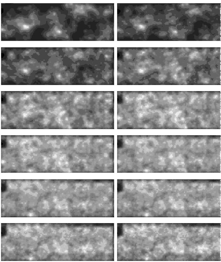
Figure 3: Greyscale Likelihood maps computed for the subregion of $338.88\leq\alpha\leq 340.84$, $-40.05\leq\delta\leq-39.46$. East is to the left and north is up. The upper left panel is the Likelihood map created for a filter redshift of $z=0.2$ and the lower right is for $z=1.3$. Each map is scaled separately, therefore the signal cannot be directly compared between the maps.

The conversion from the characteristic luminosity to the observable apparent magnitude $m^{*}$ requires an assumption to be made on the K-correction of the galaxies. Both a non-evolving galaxy model, and a model with passive evolution of the stellar population have been considered. The former is based on a template spectrum of an elliptical galaxy, taken from Coleman et al. (1980), while for the latter synthetic spectra, obtained with Bruzual and Charlot stellar population synthesis code (Bruzual & Charlot 1993), for a galaxy with solar metallicity, a star formation history with a single instantaneous burst of star formation, and a present age of 12 Gyr, were used. It is important to emphasize that the choice of a K-correction model does not significantly impact the cluster detections.

The pixel size of the Likelihood maps (i.e. the spacing between adjacent $(i,j)$ array elements) is taken to be 26.3 arcsec, corresponding to the value of the projected cluster core radius, for a cluster at a redshift of 0.6. Ideally, one would like to have a varying pixel size, corresponding to a fixed fraction of a cluster projected core radius at all filter redshifts. However this would complicate the comparison between Likelihood maps obtained with different filter redshift, and since this comparison is extremely useful for distinguishing real peaks from noise fluctuations (see Sect. 4.3), it was decided to use a fixed pixel size for the creation of the maps.

Given the typical redshift limits discussed above, 12 Likelihood maps are created from each input galaxy catalog, and these are stored as FITS-images, for ease of manipulation. Significant peaks in the likelihood distribution are identified independently in each map, using SExtractor. The mean and variance of the background are determined using a global value in each Likelihood map and peaks with more than $N_{min}$ pixels with values above the detection threshold $\sigma_{det}$ are considered as potential detections. At each filter redshift, the value of $N_{min}$ is set to correspond to the area of a circle with radius $1r_{c}$, while the value of $\sigma_{det}$ is kept constant at 2. These parameters were optimized using the simulations described in Sect. 4.3. The significance of a detection is obtained comparing the maximum value of the signal among the pixels where the likelihood is above the SExtractor detection threshold with the background noise.

The lists of peaks identified in the various Likelihood maps are then compared, and peaks detected at more than one filter redshift are associated on the basis of positional coincidence. From this association, likelihood versus $z$ curves are created, and those peaks that persist for at least three filter redshifts (Sect. 4.3) are considered as bona fide cluster candidates. The redshift and richness estimates for each candidate are derived locating the peak of the corresponding likelihood versus $z$ curve. The significance of a candidate detection is measured as the maximum of the significance versus $z$ curves regardless of the estimated redshift of the candidate cluster.

Two richness parameters are derived, following P96. The first is obtained from the matched filter procedure itself, using the parameter $\Lambda_{cl}$ introduced in equation (1). This parameter is computed using equation (29) in P96, and the Likelihood map corresponding to the cluster estimated redshift. A second independent richness estimate, $N_{R}$, is obtained to reproduce more closely the conventional Abell richness parameter: it is obtained computing the number of member galaxies (i.e. the number of galaxies above the estimated background) within a two-magnitudes interval delimited on the bright side by the magnitude of the third brightest cluster member. This galaxy is identified within a circle of radius $0.25h^{-1}$ Mpc, centered on the nominal position of the cluster detection. The magnitude distribution for all galaxies within this circle is derived using 0.20 mag bins, and the expected background contribution is subtracted from it. The background magnitude distribution is determined using the entire galaxy catalog and the same magnitude bins. Within this background-subtracted magnitude distribution the bin that contains the third brightest galaxy is identified. The entire procedure is then repeated for a circle of radius $1.0h^{-1}$ Mpc, keeping $m_{3}$, the magnitude of the third brightest galaxy, fixed to the value determined within the smaller $0.25h^{-1}$ Mpc radius circle. To reduce the probability that a foreground field galaxy on the line of sight to the cluster could bias the richness estimate, the third brightest galaxy is constrained to be fainter than $m^{*}-3$, where $m^{*}$ is computed for the cluster estimated redshift.

4.3 Tests of the Algorithm

Simulated galaxy catalogs were used to test the performance of the cluster-finding procedure and establish the best choice of extraction parameters used in the pipeline. The even and odd galaxy catalogs restricted to two smaller areas within Patch A, chosen to represent one region as uniform as possible in terms of seeing and limiting isophote, and a rather non-uniform one, were used as starting point for all simulations. From these catalogs background-only simulated galaxy catalogs were created by randomly repositioning the galaxies (within the same area), while keeping their magnitudes fixed. This procedure neglects the small correlation that is present between galaxy projected positions on the sky, but the amplitude of the galaxy-galaxy angular two-point correlation function is small enough at the magnitudes of interest here, that this approximation should have negligible impact on the simulation results.

Using these simulated catalogs it was possible to quantify the noise-rejection capabilities of the cluster finding procedure. The results obtained with the four sets of simulations (odd and even catalogs, uniform and non-uniform region) are all equivalent, and are not distinguished in the following discussion. The simulated catalogs were processed through the cluster-finding pipeline, and the peaks identification process was run a number of times, using a range of different settings for the two SExtractor detection parameters: the minimum number of pixels above the detection threshold, $N_{min}$, and the detection threshold itself, $\sigma_{det}$, expressed in units of the Likelihood map variance. It was found that noise peaks are best rejected when $N_{min}$, at all redshifts, is chosen to be roughly comparable to the area of a circle with radius the assumed cluster core radius. This is not surprising, because likelihood peaks associated with real clusters have a typical spatial scale, the one of a cluster core radius, while noise peaks do not have one. The adaptive $N_{min}$ compensates for the fixed Likelihood maps pixel scale mentioned in the previous section.

The effect of the SExtractor detection threshold on the noise detection rate is quite obvious: the higher the threshold, the fewer the noise peaks that are not rejected. However the use of a high detection threshold like $\sigma_{det}=3.0$ was found to be too restrictive, as no peaks with significance lower than 3$\sigma$ will be included in the catalog, and peaks with higher significance might also be rejected (if they fail to have $N_{min}$ pixels all above the 3$\sigma$ threshold).

Therefore other properties of the noise generated peaks were used to limit the detection when a lower threshold is used. Fig. 4 shows the distribution of the most relevant of these properties as derived using the SExtractor parameters $N_{min}=1r_{c}$ and $\sigma_{det}=2.0$. The frequency of detected peaks (scaled to a one square degree projected area) is plotted as a function of the detection significance, of the number of filter redshifts where the detection took place, and of the inferred cluster richness $\Lambda_{cl}$. From the figure it is seen that in addition to the detection significance, the number of filter redshifts at which the peak appears is a valuable tool for discriminating the noise peaks. Typically noise peaks appear at only a few filter redshifts, while clusters are detected at 5 to 10 redshifts. Therefore one further noise-rejection criterion that was enforced is the requirement that a peak should be detected over at least 3 different filter redshifts, to be included in a cluster candidates catalog. The lower panel of Fig. 4 shows another useful noise discriminant, namely the inferred richness, which for the noise peaks is rarely above 50. Therefore the requirement that the inferred richness should be $\geq 50$ has been used as a third criterion for the cluster candidate selection.

In Table 1 the results obtained applying different detection strategies to the background-only simulations are summarized. The number of detections that were found in the simulations, scaled to a common reference area of one square degree, are reported as a function of different SExtractor detection thresholds, of the adopted persistency criterion, and of the lack or presence of further restrictive criteria on the richness or the significance associated with the detection. As discussed above, while a good noise rejection can be obtained with $N_{min}\sim 1r_{c}$, $\sigma_{det}>3$ and $n_{z}>2$, this is too restrictive a setting to be used in the cluster detection procedure. At the same time a too low detection threshold ($\sigma_{det}=1.5$) results in too many blended detections. Because the automatic SExtractor de-blending procedure can override the specified $N_{min}$ criterion, it was decided not to use it, and use instead a detection threshold which does not produce a significant number of blends. Therefore the detection threshold of $\sigma_{det}=2$ was chosen. The adopted selection criteria are therefore $N_{min}\sim 1r_{c}$, $\sigma_{det}>2.0$, $n_{z}>2$, $\Lambda_{cl}>50$. This produces an expected frequency of spurious detections in the cluster candidate catalogs described in Sect. 5 of $0.2\pm 0.1$ deg^-2, if a restrictive criterion in the detection significance ($\geq 4\sigma$) is imposed, and of $1.9\pm 0.2$ deg^-2 for a detection significance $\geq 3\sigma$. For comparison, the expected frequency of spurious detections in the PDCS is 0.8 deg^-2 when peaks with significance $\geq 4\sigma$ are considered, and 4.2 deg^-2 when peaks with significance $\geq 3\sigma$ are taken into consideration.

Figure 4: The properties of noise-generated peaks in the background-only simulations. The three panels show the frequency distribution (scaled to a one square degree projected area) of noise peaks as a function of the detection significance, of the number of filter redshifts where the detection took place, and of the inferred richness. The SExtractor detection parameters used here is $N_{min}=1r_{c}$ and $\sigma_{det}=2$.

Table 1: Frequency of expected spurious detections per square degree

	$\sigma_{det}=1.5$	$\sigma_{det}=2.0$	$\sigma_{det}=3.0$
All	46.3	56.4	13.3
$n_{z}>2$	34.3	25.3	1.4
$n_{z}>2$, $\sigma\geq 3$	16.8	13.3	1.4
$n_{z}>2$, $\sigma\geq 4$	3.3	2.3	0.7
$n_{z}>2$, $\sigma\geq 3$, $\Lambda_{cl}\geq 50$	1.8	1.9	0.5
$n_{z}>2$, $\sigma\geq 4$, $\Lambda_{cl}\geq 50$	0.2	0.2	0.2

5 Results

The cluster-finding procedure described in the previous section was applied to Patch A even and odd single-frame catalogs. To facilitate a comparison between the derived cluster candidates, the search was restricted to the region of overlap between the odd/even galaxy catalogs. Furthermore, a region at the north-east corner of the patch was discarded, because of severe incompleteness (e.g., Paper I). The effective area searched is delineated in Fig. 2, covering 2.5 deg².

Using the cluster model described in Sect. 4.2 and the selection criteria described in the previous section, two cluster catalogs were constructed. One consisting of detected candidates with significance $\geq 4\sigma$, in at least one catalog (Table 2), and the other of detections having significances between $3\sigma$ and $4\sigma$ (Table 3). In both cases the additional criteria of detection requiring $n_{z}>2$ and $\Lambda_{cl}\geq 50$ are imposed. The results show that there are 15 $4\sigma$ detections in the even and 18 in the odd catalog. As shown below, most of these represent paired detections. For lower significances, one finds 13 detections in the even and 9 in the odd catalog, respectively.

For each cluster, Tables  2 and  3 give: in column (1) the cluster ID; in columns (2) and (3) the J2000 equatorial coordinates; in column (4) the estimated redshift using a K-correction obtained assuming no evolution of the stellar population; in columns (5) and (6) the richness estimates $\Lambda_{cl}$ and $N_{R}$; in columns (7) and (8) the significance for the detection in the even and odd catalog, if available; and in column (9) notes based on the visual inspection of the images of each candidate. These notes are intended to serve as an additional guide of the most likely candidates. For instance, a bright star can lead to the inclusion of spurious objects in the galaxy catalogs, which might lead to a spurious detection. When a candidate cluster is detected in both the even and odd catalogs, the redshift and richness estimates presented in the tables are the ones derived from the catalog where the highest likelihood value was measured. In total 21 $4\sigma$ candidates are reported, giving a density of 8.4 per square degree. For comparison, the density of $4\sigma$ I-band candidates in the PDCS is 6.3 per square degree. This slightly higher detection rate is probably due to a fainter limiting magnitude of the EIS catalogs (Paper I).

In Fig. 5 the projected distribution of the detected cluster candidates is shown. There is a clear paucity of clusters in the region $\alpha\leavevmode\nobreak\ \hbox to0.0pt{$>$\hss}{\lower 4.30554pt\hbox{$\sim$}}341^{\circ}$ and $\delta\leavevmode\nobreak\ \hbox to0.0pt{$>$\hss}{\lower 4.30554pt\hbox{$\sim$}}-40.2^{\circ}$. This is probably due to variations in the completeness of the single-frame catalogs at the adopted limiting magnitude of this analysis. In fact, besides the region of clear incompleteness, already removed, there is a significant area of patch A ($\sim 25\%$) which is incomplete at the magnitude adopted here (Paper I). Therefore, the definition of a more homogeneous region for the cluster analysis would require a further trimming of the effective area of the analysis. A more detailed discussion of this point will be carried out by Scodeggio et al. (1998).

Figure 5: The projected distribution of the cluster candidates. The filled circles are the $4\sigma$ candidates. Filled squares mark the paired $3\sigma$ candidates, while the open circles are the $3\sigma$ candidates detected in only one catalog.

For each cluster, cutouts from the coadded image are created centered at the nominal position of the identified cluster covering a region of $7^{\prime}\times 7^{\prime}$ area, which roughly corresponds to the FORS field of view. These cutouts are available at “http://www.eso.org/eis/datarel.html”.

Table 2: Preliminary EIS cluster catalog

Cluster name	$\alpha$ (J2000)			$\delta$ (J2000)			$z_{noevol}$	$\Lambda_{cl}$	$N_{R}$	$\sigma_{even}$	$\sigma_{odd}$	Notes
EIS 2236-3935	22	36	2.9	-39	35	33.7	0.4	64.8	9.0	5.0	5.2
EIS 2236-4017	22	36	18.0	-40	17	54.8	0.7	126.2	54.0	6.1	6.7	1
EIS 2236-4001	22	36	34.8	-40	1	57.2	0.4	56.7	21.0	5.2	5.0
EIS 2236-4026	22	36	48.6	-40	26	17.0	0.5	59.6	16.0	3.5	4.2	2, 4
EIS 2237-4000	22	37	9.1	-40	0	28.0	0.5	65.4	32.0	3.9	4.6
EIS 2238-4001	22	38	33.8	-40	1	50.6	0.7	76.3	27.0	4.0	-
EIS 2239-3957	22	39	17.3	-39	57	2.8	0.6	73.8	46.0	3.5	4.1	3
EIS 2239-3954	22	39	18.4	-39	54	34.9	0.3	65.4	37.0	6.3	7.1
EIS 2240-4020	22	40	7.8	-40	20	53.8	0.4	59.2	48.0	4.7	5.3	2
EIS 2240-4006	22	40	58.0	-40	6	27.6	0.7	74.7	45.0	4.5	3.3
EIS 2241-4001	22	41	19.0	-40	1	15.8	0.9	137.4	40.0	3.7	5.3
EIS 2241-3932	22	41	31.4	-39	32	10.4	0.5	55.9	21.0	4.0	4.3
EIS 2241-3949	22	41	42.1	-39	49	14.6	0.3	74.3	31.0	7.4	8.4
EIS 2242-4013	22	43	0.0	-40	13	55.7	0.3	55.4	17.0	6.2	5.9	4
EIS 2243-4010	22	43	1.9	-40	10	24.5	0.4	59.6	23.0	5.7	-	4
EIS 2243-3952	22	43	15.9	-39	52	12.7	0.3	79.6	19.0	6.6	7.6	3
EIS 2243-4025	22	43	21.3	-40	25	47.6	0.3	42.9	14.0	6.0	5.3
EIS 2243-3959	22	43	28.1	-39	59	31.6	0.4	63.5	26.0	-	5.5	1
EIS 2243-4014	22	43	59.6	-40	14	27.9	0.7	86.9	35.0	-	4.1	4
EIS 2244-4019	22	44	27.0	-40	19	45.2	0.4	53.8	28.0	4.8	4.5
EIS 2248-4015	22	48	53.4	-40	15	20.7	0.4	51.3	25.0	4.6	4.5

Notes to table 2 1. Detection might be affected by the presence of a bright star in the vicinity 2. Detection appears in a region of high background noise 3. Detection dominated by one bright galaxy 4. No obvious galaxy overdensity visible

Fig. 6 shows the fraction of cluster candidates found in one catalog having a counterpart in the other as function of significance. As expected, highly significant detections are found in both catalogs, within a search radius of 1 arcmin. Of the 15 $4\sigma$ detections found in the even catalog 13 (87%) have a counterpart in the odd, while for the 18 detections in the odd catalog 16 (89%) have a counterpart in the even. Note that in this comparison the counterparts may have a significance lower than $4\sigma$, but still higher than $2\sigma$ (because of the choice of the extraction threshold). It can also be seen that for $3\sigma$ detections the probability of having a counterpart in the other catalog is still reasonably high – 63% for detections in the even catalog and 74% for the odd.

Figure 6: Upper panel shows the fraction of clusters found in both catalogs as function of the significance in either the even (dotted line) or the odd (dashed line) catalog. In the lower panel the total number of detected candidates is shown for comparison.

Table 3: Additional EIS cluster candidates

Cluster name	$\alpha$ (J2000)			$\delta$ (J2000)			$z_{noevol}$	$\Lambda_{cl}$	$N_{R}$	$\sigma_{even}$	$\sigma_{odd}$	Notes
EIS 2236-3931	22	36	25.8	-39	31	13.2	0.5	55.7	11.0	3.6	-	1
EIS 2236-4008	22	36	46.0	-40	8	45.0	1.1	100.2	45.0	3.2	-	4
EIS 2236-3956	22	36	55.6	-39	56	31.0	1.3	123.6	86.0	-	3.0	4
EIS 2237-3951	22	37	38.0	-39	51	27.7	1.0	76.2	67.0	3.1	-	1
EIS 2238-4010	22	38	35.9	-40	10	36.3	0.9	81.8	36.0	3.0	-
EIS 2238-3953	22	38	46.4	-39	53	54.5	0.6	51.2	34.0	3.5	3.3
EIS 2239-3947	22	39	0.2	-39	47	7.9	0.6	63.1	48.0	3.4	-
EIS 2239-3946	22	39	34.4	-39	46	41.8	0.8	68.4	87.0	3.1	-	2, 4
EIS 2242-4018	22	42	34.8	-40	18	21.6	0.6	54.5	45.0	-	3.1
EIS 2242-3934	22	42	36.2	-39	34	16.3	0.6	74.5	25.0	3.9	-
EIS 2244-4013	22	44	57.0	-40	13	39.1	0.9	77.2	102.0	-	3.0	1, 4
EIS 2246-4011	22	46	1.3	-40	11	3.2	1.3	106.6	73.0	3.9	-	4
EIS 2246-4012	22	46	47.2	-40	12	48.5	0.5	52.2	27.0	3.4	3.6
EIS 2247-4025	22	47	40.2	-40	25	55.8	1.3	96.1	39.0	-	3.1	2, 4
EIS 2248-3951	22	48	29.8	-39	51	26.2	0.6	62.7	27.0	3.5	3.6
EIS 2249-3958	22	49	31.7	-39	58	12.5	0.9	76.4	29.0	-	3.0
EIS 2249-4016	22	49	32.5	-40	16	36.1	0.7	76.8	41.0	3.6	3.8
EIS 2249-4021	22	49	46.6	-40	21	49.9	1.3	87.5	82.0	3.2	-	4

Notes to table 3 1. Detection might be affected by the presence of a bright star in the vicinity 2. Detection appears in a region of high background noise 3. Detection dominated by one bright galaxy 4. No obvious galaxy overdensity visible

The estimated redshifts for the detected clusters range between $z=0.3$ and $z=1.3$. In Fig. 7 the redshift distribution of the total candidate sample is shown and compared to the distribution for the candidates reported in the PDCS. The shaded area represents the redshift distribution of the $4\sigma$ candidates.

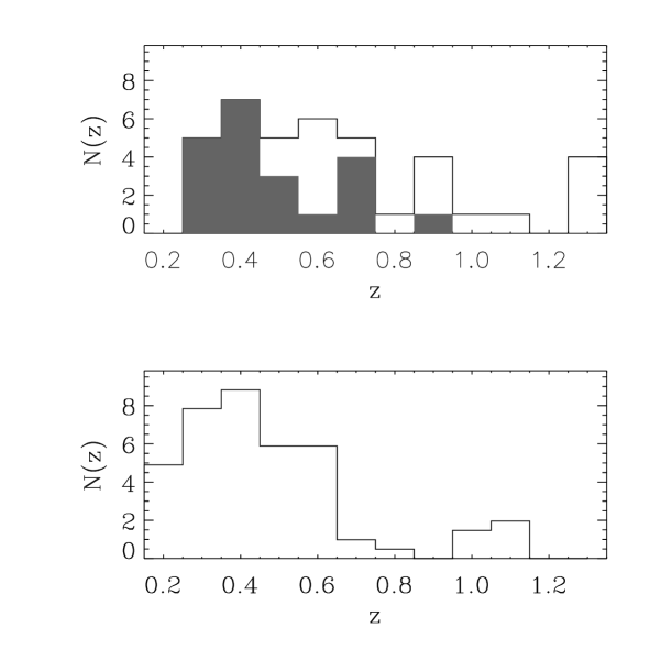
Figure 7: The upper panel shows the redshift distribution of the cluster candidates in Tables 2 and 3. The shaded area is the distribution of the good clusters while the white area shows the additional contribution from the less robust candidates. The lower panel shows the redshift distribution for the cluster candidates from the PDCS scaled to an area of 2.5deg^-2 for comparison.

The distribution of the $4\sigma$ candidates is seen to cover the redshift range from 0.3 to 0.9 with a median redshift of $z=0.4$, while the total sample extends to $z=1.3$ with a median of $z=0.6$. For comparison, the median redshift of the PDCS is $z=0.4$. The EIS and PDCS redshift distributions are quite similar, but a small relative shift in redshift may be present. This effect might be either due to a small bias of the current implementation of the matched filter algorithm or to the fact that the EIS data are somewhat deeper than those of the PDCS.

Applying the passive evolution K-corrections in the creation of the Likelihood maps, in most cases, does not affect the detection of a candidate. However, there are a few cases where the candidates detected with the no-evolution K-corrections fail to be detected with the passive evolution K-corrections.

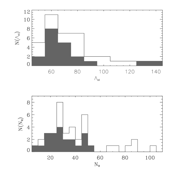
Figure 8: The upper panel shows the distribution of the richness measure $\Lambda_{cl}$, the shaded area is the distribution of the good candidates and the white shows the additional contributions from the less robust candidates. The lower panel shows the distribution of Abell-richness.

The distributions of estimated cluster richness are shown in Fig. 8. Again the distributions for the total cluster sample is shown, and the shaded area indicates the distribution for the $4\sigma$ candidates. It is seen that the $\Lambda_{cl}$ richness spans a wide range extending up to $\sim 140$ with a median of $\sim 70$. The Abell richness estimate, $N_{R}$, is found to vary between 9 and 102 with a median of 34. Note that in the case of richness an appropriate comparison with the results of P96 cannot be made because of our imposed richness criterion in the detection and differences between the estimates of the mean background counts in the calculation of the Abell richness in this paper and PDCS.

A comparison between the estimates of the candidates properties, discussed in the previous section, is used to obtain a rough estimate of their accuracy. Fig.  9 shows a comparison of the estimated redshifts for all paired detections, as determined in the odd/even catalogs. Some of the points represent more than one cluster candidate due to the discreteness of the redshift bins. The scatter around the diagonal is found to be $\sim$ 0.06, consistent with the possible accuracy given by the adopted redshift grid. In Fig. 10 the richness estimates are compared in the same way and it is found that for $\Lambda_{cl}$ the scatter is 21% and for $N_{R}$ the scatter is 39%.

Figure 9: The redshifts derived from the even and odd catalogs are compared. Some points represents more than one detection. The scatter around the diagonal is 0.06.

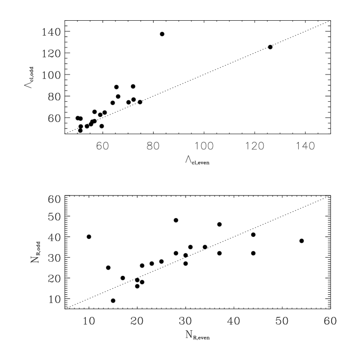
Figure 10: The upper panel shows a comparison between the richness, $\Lambda_{cl}$ as derived from the even and odd catalogs. It is seen that there is good agreement between the two catalogs with a scatter of about 21%. The lower panel shows a comparison of the Abell richness, which also shows good agreement though with a larger scatter of 39%.

6 Summary and Future developments

The recently released EIS I-band data for Patch A ($\alpha\sim 22^{h}45^{m}$ and $\delta\sim-40^{\circ}$; see Paper I) have been used to search for clusters of galaxies over an area of 2.5 square degrees, in the redshift range $0.2\leq z\leq 1.3$. The matched filter algorithm has been applied to the even and odd single-frame catalogs to assess the performance of the detection technique, to establish the detection threshold for robust detections and to evaluate the quality of the EIS data for this kind of analysis, one of the main goals of the survey.

The candidate cluster sample based on of $4\sigma$ detections consists of 21 objects, yielding a surface density of 8.4 candidates per square degree, with a median redshift of $z=0.4$. When all $3\sigma$ detections are considered 39 candidates are found, leading to a surface density of 16 per square degree and a median redshift of $z=0.6$. Cutouts for the cluster candidates are available at “http://www.eso.org/eis/datarel.html”. These results should be considered preliminary as significantly better data are available for the other EIS patches. More importantly, the use of catalogs extracted from the coadded images will allow a deeper cluster search to be carried out, thereby extending the redshift range for the cluster sample. Clearly, the EIS data more than fulfills the science requirements of the survey, as originally stated.

In this first release of the EIS cluster catalog the effort has been concentrated on the I-band data. However, a limited number of frames in V-band have been obtained and will be used to further investigate the candidate clusters over the surveyed region (Olsen et al. 1998). The present study will be extended to include detailed simulations to establish the intrinsic accuracy of the method used here and to eventually derive the selection function for the cluster catalog.

- (1) Bruzual, A.G., Charlot, S. 1993, ApJ, 405, 538
- (2) Coleman, G.D., Wu,C.-C., Weedman, D.W. 1980 ApJS, 43, 393
- (3) Connolly, A.J., Szalay, A.S., Koo, D., Romer, A.K., Holden,B., Nichol, R.C., Miyaji, T. 1996, ApJ, 473, L67
- (4) Couch, W.J., Ellis, R.S., MacLaren, I., Malin, D.F. 1991, MNRAS, 249, 606
- (5) Dalcanton, J.J. 1996, ApJ, 466, 92
- (6) Deltorn, J.-M., Le Fevre, O., Crampton, D., Dickinson, M. 1997, ApJ, 483, L21
- (7) Dickinson, M. 1995, in “Fresh Views of Elliptical Galaxies”, A. Buzzoni, A. Renzini, A. Serrano eds., (ASP: San Francisco) p. 283
- (8) D’Odorico, S. 1990, Messenger, 61, 51
- (9) Francis, P.J., et al. 1996, ApJ, 457, 490
- (10) Gioia, I.M., Luppino, G.A. 1994, ApJS, 94, 583
- (11) Gunn, J.E., Hoessel, J.G., Oke, J.B. 1986, ApJ, 306, 30
- (12) Henry, J.P., Gioia, I.M., Mullis, C.R., Clowe, D.I., Luppino, G.A., Boehringer, H., Briel, U.G., Voges, W., Huchra, J.P. 1997, AJ, 114, 1293
- (13) Kawasaki, W., Shimasaku, K., Doi, M., Okamura, S. 1997, astro-ph/9705112
- (14) Lidman, C.E., Peterson, B.A. 1996, AJ, 112, 2454
- (15) Nonino, M., et al. 1998, submitted to A&A; astro-ph/9803336 (Paper I)
- (16) Olsen, L.F., et al. 1998, in preparation
- (17) Pascarelle, S.M., Windhorst, R.A., Driver, S.P., Ostrander, E.J., Keel, W.C. 1996, ApJ, 456, L21
- (18) Postman, M., Lubin, L.M., Gunn, J.E., Oke, J.B., Hoessel, J.G., Schneider, D.P., Christensen, J.A. 1996, AJ, 111, 615 (P96)
- (19) Renzini, A., da Costa, L. N. 1997, Messenger 87, 23
- (20) Rosati, P., Della Ceca, R., Norman, C., Giacconi, R. 1998, ApJ, 492, L21
- (21) Schechter, P. 1976, ApJ, 203, 557
- (22) Scodeggio, M., et al. 1998, in preparation
- (23) Stanford, S.A., Elston, R., Eisenhardt, P.R., Spinrad, H., Stern, D., Dey, A. 1997, AJ, 114, 2232
- (24) Zaritsky, D., Nelson, A.E., Dalcanton, J.J., Gonzalez, A.H. 1997, ApJ, 480, L91