ON THE EVOLUTION OF THE COSMIC SUPERNOVA RATES
Abstract
Ongoing searches for supernovae (SNe) at cosmological distances have recently started to provide a link between SN Ia statistics and galaxy evolution. We use recent estimates of the global history of star formation to compute the theoretical Type Ia and Type II SN rates as a function of cosmic time from the present epoch to high redshifts. We show that accurate measurements of the frequency of SN events in the range will be valuable probes of the nature of Type Ia progenitors and the evolution of the stellar birthrate in the universe. The Next Generation Space Telescope should detect of order 20 Type II SNe per field per year in the interval .
keywords:
galaxies: evolution – supernovae: general1 Introduction
The remarkable progress in our understanding of faint galaxy data made possible by the combination of HST deep imaging (Williams et al. 1996) and ground-based spectroscopy (Lilly et al. 1995; Ellis et al. 1996; Cowie et al. 1996; Steidel et al. 1996), has recently permitted to shed some light on the evolution of the stellar birthrate in the universe, to identify the epoch where most of the optical extragalactic background light was produced, and to set important contraints on galaxy formation scenarios (Madau et al. 1998; Steidel et al. 1998). While one of the biggest uncertainties in our knowledge of the emission history of the universe is probably represented by the poorly constrained amount of starlight that was absorbed by dust and reradiated in the IR at early and late epochs, one could also imagine the existence of a large population of relatively old or faint galaxies still undetected at high-, as the color-selected ground-based and Hubble Deep Field samples include only the most actively star-forming young objects. It is then important at this stage to devise different observational strategies, free of some of the biases that plague current galaxy surveys, and to make testable predictions for future astronomical capabilities, such as SIRTF, FIRST and NGST.
Here, we shall focus our attention on the rate of supernova (SN) explosions in the universe. An obvious reason to consider SNe is purely observational, i.e. the fact that they are very bright objects, with luminosities as high as , and are point-like sources, making their detection possible even at very large distances/redshifts. More in general, the evolution of the SN rate with redshift contains unique information on the star formation history of the universe, the initial mass function (IMF) of stars, and the nature of the binary companion in Type Ia events. All are essential ingredients for understanding galaxy formation, cosmic chemical evolution, and the mechanisms which determined the efficiency of the conversion of gas into stars in galaxies at various epochs (e.g. Madau et al. 1996; Madau, Pozzetti, & Dickinson 1997; Renzini 1997). While the frequency of “core-collapse supernovae”, SN II and possibly SN Ib/c, which have short-lived progenitors (e.g. Wheeler & Swartz 1993) is essentially related, for a given IMF, to the instantaneous stellar birthrate of massive stars, Type Ia SNe – which are believed to result from the thermonuclear disruption of C-O white dwarfs in binary systems – follow a slower evolutionary clock, and can then be used as a probe of the past history of star formation in galaxies (e.g. Branch et al. 1995; Ruiz-Lapuente, Canal, & Burkert 1997; Yungelson & Livio 1998). The recent detection of Type Ia SNe at cosmological distances (Kim et al. 1997; Garnavich et al. 1998; Perlmutter et al. 1998) allow for the first time a detailed comparison between the SN rates self-consistently predicted by stellar evolution models that reproduce the optical spectrophotometric properties of field galaxies, and the observed values.
In this Letter we show how accurate measurements at low and intermediate redshifts of the frequencies of Type II(+Ib/c) and Ia SNe could be used as an independent test for the star formation and heavy element enrichment history of the universe, and significantly improve our understanding of the intrinsic nature and age of the populations involved in the SN explosions. A determination of the amount of star formation at early epochs is of crucial importance, as the two competing scenarios for galaxy formation, monolithic collapse – where spheroidal systems formed early and rapidly, experiencing a bright starburst phase at high- (Eggen, Lynden-Bell, & Sandage 1962; Tinsley & Gunn 1976) – and hierarchical clustering – where ellipticals form continuosly by the merger of disk/bulge systems (White & Frenk 1991; Kauffmann et al. 1993) and most galaxies never experience star formation rates in excess of a few solar masses per year (Baugh et al. 1998) – appear to make rather different predictions in this regard. We show how, by detecting Type II SNe at high-, the Next Generation Space Telescope should provide an important test for distinguishing between different scenarios of galaxy formation.
2 Basic Theory
2.1 Cosmic Star Formation History
In this section we shall follow Madau et al. (1998), and model the emission history of field galaxies at ultraviolet, optical, and near-infrared wavelengths by tracing the evolution with cosmic time of their luminosity density,
| (1) |
where is the best-fit Schechter luminosity function in each redshift bin. The integrated light radiated per unit volume from the entire galaxy population is an average over cosmic time of the stochastic, possibly short-lived star formation episodes of individual galaxies, and follows a relatively simple dependence on redshift. Madau et al. (1998) have shown how a stellar evolution model, defined by a time-dependent star formation rate per unit volume, , a universal IMF, , and some amount of reddening, can actually reproduce the optical data reasonably well. In such a system, the luminosity density at time is given by the convolution integral
| (2) |
where is the specific luminosity radiated per unit initial mass by a generation of stars with age , and is a time-independent term equal to the fraction of emitted photons which are not absorbed by dust, in a foreground screen model. The function is derived from the observed UV luminosity density, and is then used as input to the population synthesis code of Bruzual & Charlot (1998).
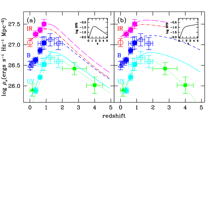
Figure 1a shows the model predictions for the evolution of for a Salpeter (1955) function (), with SMC-type dust (in this case, the observed UV luminosities must be corrected upwards by a factor of 1.4 at 2800 Å and 2.1 at 1500 Å), and a star formation history which traces the rise, peak, and sharp drop of the UV emissivity. 111A convenient fit to 5% accuracy to the star formation history used for Figure 1a is , where is the Hubble time in Gyr, . Note that, although in our calculations the IMF extends down to , stars below 0.8 make only a small contribution to the emitted near-IR light. This introduces a non-negligible uncertainty in our estimates of the total stellar birthrate. For example, in the case of a Salpeter IMF with , the inferred star formation rate, , would decrease by a factor of 1.88. For simplicity, the metallicity was fixed to solar values and the IMF truncated at 0.1 and 125 : none of these assumptions is crucial for our results. The data points show the observed luminosity density in six broad passbands centered around 0.15, 0.20, 0.28, 0.44, 1.0, and 2.2 µm. The model is able to account for the entire background light recorded in the galaxy counts down to the very faint magnitude levels probed by the Hubble Deep Field (HDF), and produces visible mass-to-light ratios at the present epoch which are consistent with the values observed in nearby galaxies of various morphological types. The bulk ( by mass) of the stars present today formed relatively recently (), consistently with the expectations from a broad class of hierarchical clustering cosmologies (Baugh et al. 1998), and in good agreement with the low level of metal enrichment observed at high redshifts in the damped Lyman- systems (Pettini et al. 1997).
One of the biggest uncertainties in our understanding of the evolution of luminous matter in the universe is represented by the poorly constrained amount of starlight that was absorbed by dust and reradiated in the far-IR at early epochs. While the Salpeter IMF, SMC-dust model reproduces quite well the rest-frame UV colors of high- objects in the HDF, the prescription for a “correct” de-reddening of Lyman-break galaxies is the subject of an ongoing debate (see Pettini et al. 1998 and references therein). Figure 1b shows the model predictions for a monolithic collapse scenario, where half of the present-day stars – the fraction contained in spheroidal systems (Schechter & Dressler 1987) – were formed at and were enshrouded by dust.222A fitting formula to the stellar birthrate used for Figure 1b is to 1% accuracy. Consistency with the HDF “dropout” analysis has been obtained assuming a dust extinction which increases rapidly with redshift, . This results in a correction to the rate of star formation by a factor of and 15 at and 4, respectively. The model is still consistent with the global history of light, but overpredicts the metal mass density at high redshifts as sampled by QSO absorbers. In order for such a model to be acceptable, the gas traced by the damped Lyman- systems would have to be physically distinct from the luminous star forming regions observed in high- galaxies, and to be substantially under-enriched in metals compared to the cosmic mean.
In the next section we shall compute the expected evolution with cosmic time of the Type Ia and II/Ib,c supernova frequencies for the two star formation histories – for brevity, we shall refer to them as the “merging” versus “monolithic collapse” scenarios – discussed above. By focusing on the integrated light radiated by the galaxy population as a whole, our approach will not specifically address the evolution and the SN rates of particular subclasses of objects, like the oldest ellipticals or low-surface brightness galaxies, whose star formation history may have differed significantly from the global average.
2.2 Type Ia and II(+Ib/c) Supernova Rates
Single stars with mass evolve rapidly ( Myr) through all phases of central nuclear burning, ending their life as Type II SNe with different characteristics depending on the progenitor mass (e.g. Iben & Renzini 1983). For a Salpeter IMF (with lower and upper mass cutoffs of 0.1 and 125 ), the core-collapse supernova rate can be related to the stellar birthrate according to
| (3) |
It is worth noting at this stage that our model predictions for the frequency of Type II events are largely independent of the assumed IMF. This follows from the fact that the rest-frame UV continuum emission – which is used as an indicator of the instantaneous star formation rate – from all but the oldest galaxies is entirely dominated by massive stars on the main sequence, the same stars which later give origin to a core collapse SN.
The specific evolutionary history leading to a Type Ia event remains instead an unsettled question. SN Ia are believed to result from the explosion of C-O white dwarfs (WDs) possibly triggered by the accretion of material from a companion, the nature of which is still unknown (see Ruiz-Lapuente et al. 1997 for a recent review). In a double degenerate (DD) system, for example, such elusive companion is another WD: the exploding WD reaches the Chandrasekhar limit and carbon ignition occurs at its center (Iben & Tutukov 1984). In the single degenerate (SD) model instead, the companion is a nondegenerate, evolved star that fills its Roche lobe and pours hydrogen or helium onto the WD (Whelan & Iben 1973; Iben & Tutukov 1984). While in the latter the clock for the explosion is set by the lifetime of the primary star and, e.g., by how long it takes to the companion to evolve and fill its Roche lobe, in the former it is controlled by the lifetime of the primary star and by the time it takes to shorten the separation of the two WDs as a result of gravitational wave radiation. The evolution of the rate depends then, among other things, on the unknown mass distribution of the secondary binary components in the SD model, or on the distribution of the initial separations of the two WDs in the DD model.
To shed light into the identification issue and, in particular, on the clock-mechanism for the explosion of Type Ia’s, we shall adopt here a more empirical approach. We choose to parametrize the rate of Type Ia’s in terms of a characteristic explosion timescale, – which defines an explosion probability per WD assumed to be independent of time – and an explosion efficiency, . The former accounts for the time it takes in the various models to go from a newly born (primary) WD to the SN explosion itself: a spread of “delay” times results from the combination of a variety of initial conditions, such as the mass ratio of the binary system, the distribution of initial separations, the influence of metallicity on the mass transfer rate and accretion efficiency, etc., folded with the various possible mechanisms that lead to a Type Ia event. The latter simply accounts for the fraction of stars in binary systems that, because of unfavorable initial conditions, will never undergo a SN Ia explosion. We consider as possible progenitors all systems in which the primary star has an initial mass higher than (final mass , Weidemann 1987) and lower than (cf Greggio & Renzini 1983): stars less massive than will not produce a catastrophic event even if the companion has comparable mass, while stars more massive than will undergo core collapse, generating a Type II explosion.
With these assumptions the rate of Type Ia events at any one time will be given by the sum of the explosions of all the binary WDs produced in the past that have not had the time to explode yet, i.e.
| (4) |
where , is the minimum mass of a star that reaches the WD phase at time , and is the standard lifetime of a star of mass (all stellar masses are expressed in solar units). For a fixed initial mass , the frequency of Type Ia events peaks at an epoch that reflect an “effective” delay from stellar birth. A prompter (smaller ) explosion results in a higher SN Ia rate at early epochs.
3 Comparison with the Data
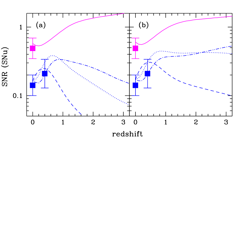
Observed rates of SNe are normally given in units of SNu, one SNu corresponding to 1 SN per 100 years per . Since a galaxy luminosity depends on , there is a factor involved in the inferred SN frequencies. The typical uncertainties on the present-day rates are summarized in Table 1, where we have reported the determinations of Cappellaro et al. (1997), Tammann, Löffler, & Schröder (1994), and Evans, van den Bergh, & McClure (1989). These agree to within a factor of 3 for Type Ia in early type galaxies and Type Ib/c in spirals, and to within a factor of 2 for Type II in late spirals. The “internal” error in each entry is of order . When weighted according to the local blue luminosity function by spectral type of Heyl et al. (1997) (which assigns about 28% of the total local blue luminosity density to elliptical galaxies, 32% to early spirals, and 40% to late spirals), the tabulated frequencies yield a mean – averaged over the entire galaxy population – SN Ia rate of (0.12,0.19,0.12) SNu, and a SN II(+Ib/c) rate of (0.32,0.62,0.60) SNu (the three values corresponding to the measurements of Cappellaro et al. 1997, Tammann et al. 1994, and Evans et al. 1989, respectively). A simple geometric mean of these determinations gives the values, SNu and SNu, we shall adopt for comparison with the theoretical rates. At higher redshifts, searches for SNe have been pioneered by Hansen et al. (1989) and Norgaard-Nielson et al. (1989). Recently, systematic searches of distant SNe (Kim et al. 1997; Garnavich et al. 1998; Perlmutter et al. 1998) have provided the first measurement of the rate of Type Ia at , SNu (Pain et al. 1997).
In Figure 2 we show the predicted Type Ia and II(+Ib/c) rest-frame frequencies as a function of redshift. Expressed in SNu, the Type II rate is basically proportional to the ratio between the UV and blue galaxy luminosity densities, and is therefore independent of cosmology. Unlike the SN frequency per unit volume, which will trace the evolution of the stellar birthrate, the frequency of Type II events per unit blue luminosity is a monotonic increasing function of redshift, and depends only weakly on the assumed star formation history. The Type Ia rates plotted in the figure assume characteristic “delay” timescales after the collapse of the primary star to a WD equal to and 3 Gyr, which virtually encompass all relevant possibilities. The SN Ia explosion efficiency was left as an adjustable parameter to reproduce the observed ratio of SN II to SN Ia explosion rates in the local universe, , for the adopted models.
It appears that observational determinations of the SN Ia rate at can unambiguously identify the appropriate delay time. In particular, we estimate that measuring the frequency of Type Ia events at both and with an error of 20% or lower would allow one to determine this timescale to within about 30%. This kind of observations are by no means prohibitive, and these goals could be achieved within a couple of years. In fact, ongoing searches for high- SNe (Perlmutter et al. 1998; Garnavich et al. 1998) are currently able to discover and study about a dozen new events per observing session in the redshift range 0.4-1.0, and the observations are carried out at a rate of about four sessions a year. Since determining the frequency of SN Ia with a 20% uncertainty requires statistics on more than 25 objects per redshft bin, it is clear that, barring systematic biases, those rates will soon be know with high accuracy. Also note how, relative to the merging scenario, the monolithic collapse model predicts Type Ia rates (in SNU) that are, in the Gyr case, a factor of 1.6 and 4.9 higher at and 4, respectively, with even larger factors found in the case of longer delays. Therefore, once such timescale is calibrated through the observed ratio SNRSNR, one should be able to constrain the star formation history of the early universe by comparing the predicted SN Ia rate at with the observations.
4 Conclusions
We have investigated the link between SN statistics and galaxy evolution. Using recent determinations of the star formation history of field galaxies from the present epoch to high-, and a simple model for the evolutionary history of the binary system leading to a Type Ia event, we have computed the theoretical Type Ia and Type II SN rates as a function of cosmic time. While significant uncertainties still remain in these estimates, we believe the calculations presented in this Letter offer a first, realistic glimpse to the evolution of the cosmic supernova rates with cosmic time. Our main results can be summarized as follows.
-
•
At the present epoch, the predicted Type II(+Ib/c) frequency appears to match remarkably well the observed local value. The obvious caveat is the well known fact that the SN II rate is a sensitive function of the lower mass cutoff of the progenitors, . Values as low as (Chiosi, Bertelli, & Bressan 1992) or as high as (Nomoto 1984) have been proposed in the literature: adopting a lower mass limit of 6 or 11 would increase or reduce our Type II rates by a factor 1.5, respectively. Note also that rates obtained from traditional distant (beyond 4 Mpc) sample might need to be increased by a factor of 1.5–2 because of severe selection effects against Type II’s fainter than (Woltjer 1997).
-
•
In the interval , the predicted rate of SN Ia is a sensitive function of the characteristic delay timescale between the collapse of the primary star to a WD and the SN event. Accurate measurements of SN rates in this redshift range will improve our understanding of the nature of SN Ia progenitors and the physics of the explosions. Ongoing searches and studies of distant SNe should soon provide these rates, allowing a universal calibration of the Type Ia phenomenon.
-
•
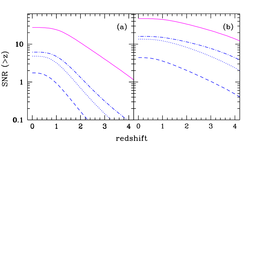
While Type Ia rates at will offer valuable information on the star formation history of the universe at earlier epoch, the full picture will only be obtained with statistics on Type Ia and II SNe at redshifts or higher. At these epochs, the detection of Type II events must await the Next Generation Space Telescope (NGST). A SN II has a typical peak magnitude (e.g. Patat et al. 1994): placed at , such an explosion would give rise to an observed flux of 15 nJy (assuming a flat cosmology with and ) at 1.8 µm. At this wavelength, the imaging sensitivity of an 8m NGST is 1 nJy ( s exposure and detection threshold), while the moderate resolution () spectroscopic limit is about 50 times higher ( s exposure per resolution element and detection threshold) (Stockman et al. 1998). The several weeks period of peak rest-frame blue luminosity would be stretched by a factor of to few months. Figure 3 shows the cumulative number of Type II events expected per year per field. Depending on the history of star formation at high redshifts, the NGST should detect between 7 (in the merging model) and 15 (in the monolithic collapse scenario) Type II SNe per field per year in the interval . The possibility of detecting Type II SNe at from an early population of galaxies has been investigated by Miralda-Escudé & Rees (1997). By assuming these are responsible for the generation of all the metals observed in the Lyman- forest at high redshifts, a high baryon density (), and an average metallicity of , Miralda-Escudé & Rees estimate the NGST should observe about 16 SN II per field per year with . Note, however, that a metallicity smaller by a factor compared to the value adopted by these authors has been recently derived by Songaila (1997). For comparison, the models discussed in this Letter predict between 1 and 10 Type II SNe per field per year with .
Acknowledgements.
PM acknowledges support from NASA through ATP grant NAG5-4236. MDV thanks the ospitality of the STScI, where part of this work was done.References
- (1) Baugh, C. M., Cole, S., Frenk, C. S., & Lacey, C. G. 1998, ApJ, in press (astro-ph/9703111)
- (2) Branch, D., Livio, M., Yungelson, L. R., Boffi, F., & Baron, E. 1995, PASP, 107, 1
- (3) Bruzual, A. G., & Charlot, S. 1998, in preparation
- (4) Cappellaro, E., Turatto, M., Tsvetkov, D. Yu., Bartunov, O. S., Pollas, C., Evans, R., & Hamuy, M. 1997, A&A, 322, 431
- (5) Chiosi, C., Bertelli, G., & Bressan, A. 1992, ARA&A, 30, 235
- (6) Connolly, A. J., Szalay, A. S., Dickinson, M. E., SubbaRao, M. U., & Brunner, R. J. 1997, ApJ, 486, L11
- (7) Cowie, L. L., Songaila, A., Hu, E. M., & Cohen, J. G. 1996, AJ, 112, 839
- (8) Eggen, O. J., Lynden-Bell, D., & Sandage, A. R. 1962, ApJ, 136, 748
- (9) Ellis, R. S., Colless, M., Broadhurst, T., Heyl, J., & Glazebrook, K. 1996, MNRAS, 280, 235
- (10) Evans, R., van den Bergh, S., & McClure, R.D. 1989, ApJ, 345, 752
- (11) Gardner, J. P., Sharples, R. M., Frenk, C. S., & Carrasco, B. E. 1997, ApJ, 480, L99
- (12) Garnavich, P. M., et al. 1998, ApJ, 493, L53
- (13) Greggio, L., & Renzini, A. 1983, A&A, 118, 217
- (14) Hansen, L., Jorgensen, H. E., Norgaard-Nielsen, H. U., Ellis, R. S., & Couch, W. J. 1989, A&A, 211, L9
- (15) Heyl, J., Colless, M., Ellis, R. S., & Broadhurst, T. 1997, MNRAS, 285, 613
- (16) Iben, I. Jr., & Renzini, A. 1983, ARA&A, 21, 271
- (17) Iben, I. Jr., & Tutukov, A. 1984, ApJS, 54, 535
- (18) Kauffmann, G., White, S. D. M., & Guiderdoni, B. 1993, MNRAS, 264, 201
- (19) Kim, A. G., et al. 1997, ApJ, 476, L63
- (20) Lilly, S. J., Le Févre, O., Hammer, F., & Crampton, D. 1996, ApJ, 460, L1
- (21) Lilly, S. J., Tresse, L., Hammer, F., Crampton, D., & Le Févre, O. 1995, ApJ, 455, 108
- (22) Madau, P. 1997, in Star Formation Near and Far, ed. S. S. Holt & G. L. Mundy, (AIP: New York), p. 481
- (23) Madau, P., Ferguson, H. C., Dickinson, M. E., Giavalisco, M., Steidel, C. C., & Fruchter, A. 1996, MNRAS, 283, 1388
- (24) Madau, P., Pozzetti, L., & Dickinson, M. E. 1998, ApJ, in press (astro-ph/9708220)
- (25) Miralda-Escudé, J., & Rees, M. J. 1997, ApJ, 478, L57
- (26) Nomoto, K. 1984, ApJ, 277, 791
- (27) Norgaard-Nielsen, H. U., Hansen, L., Jorgensen, H. E., Aragón-Salamanca, A., & Ellis, R. S. 1989, Nature, 339, 523
- (28) Pain, R., et al. 1997, ApJ, 473, 356
- (29) Patat, R., Barbon, R., Cappellaro, E. Turatto, M. 1994, A&A, 282, 731
- (30) Perlmutter, S., et al. 1998, Nature, 391, 51
- (31) Pettini, M., Smith, L. J., King, D. L., & Hunstead, R. W. 1997, ApJ, 486, 665
- (32) Pettini, M., Steidel, C. C., Dickinson, M., Kellogg, M., Giavalisco, M., & Adelberger, K. L. 1998, in The Ultraviolet Universe at Low and High Redshift, ed. W. Waller, (Woodbury: AIP Press), in press (astro-ph/9707200)
- (33) Renzini, A. 1997, ApJ, 488, 35
- (34) Ruiz-Lapuente, P., Canal, R., & Burkert, A. 1997, in Thermonuclear Supernovae, ed. P. Ruiz-Lapuente, R. Canal, & J. Isern (Dordrecht: Kluwer), p. 205
- (35) Salpeter, E. E. 1955, ApJ, 121, 161
- (36) Schechter, P. L., & Dressler, A. 1987, AJ, 94, 56
- (37) Songaila, A. 1997, ApJ, 490, L1
- (38) Steidel, C. C., Adelberger, K. L., Dickinson, M. E., Giavalisco, M., Pettini, M., & Kellogg, M. 1998, ApJ, 492, 428
- (39) Steidel, C. C., Giavalisco, M., Pettini, M., Dickinson, M. E., & Adelberger, K. L. 1996, ApJ, 462, L17
- (40) Stockman, H. S., Stiavelli, M., Im, M., & Mather, J. C. 1998, in Science with the Next Generation Space Telescope, ed. E. Smith & A. Koratkar (ASP Conf. Ser.), in press
- (41) Tammann, G. A., Löffler, W., & Schröder, A. 1994, ApJS, 92, 487
- (42) Tinsley, B. M., & Gunn, J. E. 1976, ApJ, 203, 52
- (43) Treyer, M. A., Ellis, R. S., Milliard, B., & Donas, J. 1998, in The Ultraviolet Universe at Low and High Redshift, ed. W. Waller, (Woodbury: AIP Press), in press (astro-ph/9706223)
- (44) van den Bergh, S., & Tammann, G. A. 1991, ARA&A, 29, 363
- (45) Weidemann, V. 1987, A&A, 188, 74
- (46) Wheeler, J. C., & Swartz, D. A. 1993, Space Sci. Rev., 66, 425
- (47) Whelan, J., & Iben, I. Jr. 1973, ApJ, 186, 1007
- (48) White, S. D. M., & Frenk, C. S. 1991, ApJ, 379, 25
- (49) Williams, R. E., et al. 1996, AJ, 112, 1335
- (50) Woltjer, L. 1997, A&A, 328, L29
- (51) Yungelson, L., & Livio, M. 1998, ApJ, in press (astro-ph/9711201)
- (52)
| Hubble Type | Ia | Ib/c | II |
|---|---|---|---|
| E–S0 | 0.07, 0.25, 0.08 | ||
| S0a–Sa | 0.11, 0.12, 0.15 | 0.07, 0.01, | 0.07, 0.04, |
| Sab–Sb | 0.08, 0.12, 0.08 | 0.04, 0.07, 0.15 | 0.24, 0.34, 0.45 |
| Sbc–Sd | 0.11, 0.12, 0.05 | 0.07, 0.19, 0.18 | 0.39, 0.98, 0.58 |