Microlensing by Multiple Planets in High Magnification Events

Abstract

Microlensing is increasingly gaining recognition as a powerful method for the detection and characterization of extra-solar planetary systems. Naively, one might expect that the probability of detecting the influence of more than one planet on any single microlensing light curve would be small. Recently, however, Griest & Safizadeh (1998) have shown that, for a subset of events, those with minimum impact parameter $u_{min}{{}_{<}\atop{}^{{}^{\sim}}}0.1$ (high magnification events), the detection probability is nearly 100% for Jovian mass planets with projected separations in the range 0.6–1.6 of the primary Einstein ring radius $R_{E}$, and remains substantial outside this zone. In this Letter, we point out that this result implies that, regardless of orientation, all Jovian mass planets with separations near 0.6–1.6$R_{E}$ dramatically affect the central region of the magnification pattern, and thus have a significant probability of being detected (or ruled out) in high magnification events. The probability, averaged over all orbital phases and inclination angles, of two planets having projected separations within $0.6$–$1.6R_{E}$ is substantial: 1-15% for two planets with the intrinsic orbital separations of Jupiter and Saturn orbiting around 0.3–1.0$M_{\odot}$ parent stars. We illustrate by example the complicated magnification patterns and light curves that can result when two planets are present, and discuss possible implications of our result on detection efficiencies and the ability to discriminate between multiple and single planets in high magnification events.

submitted to the Astrophysical Journal Letters: March 24, 1998

1 Introduction

A planetary microlensing event occurs whenever the presence of a planet creates a perturbation to the standard microlensing event light curve. These perturbations typically have magnitudes of ${{}_{<}\atop{}^{{}^{\sim}}}20\%$ and durations of a few days or less. First suggested by Mao & Paczyński (1991) as a method to detect extra-solar planetary systems, the possibility was explored further by Gould & Loeb (1992), who found that roughly 15% of microlensing light curves should show evidence of planetary deviations if all primary lenses have Jupiter-mass planets with orbital separations comparable to that of Jupiter. Although these probabilities are relatively high, the use of microlensing to discover planets was largely ignored since in order to detect the primary events the microlensing survey teams must monitor millions of stars in very crowded fields, resulting in temporal sampling that is too low ($\sim 1\,{\rm day}$) and photometric errors that are too high (${{}_{>}\atop{}^{{}^{\sim}}}5\%$) to detect most secondary planetary deviations (Alcock et al. 1997a).

Recently, the situation has changed dramatically as the real-time reduction of the survey teams has enabled them to issue electronic “alerts,” notification of on-going events detected before the peak magnification (Udalski et al. 1994, Pratt et al. 1996), allowing other collaborations to perform special purpose observations of the alerted events. These additional observations include denser photometric sampling by the PLANET and GMAN collaborations (Albrow et al. 1996, 1997, 1998 and Pratt et al. 1996, Alcock et al. 1997b) as well as spectroscopic follow-up of particular events (Lennon et al. 1997). Over 60 events are currently alerted per year towards the Galactic Bulge. Since only a handful of these are on-going at any given time, monitoring teams can sample events very densely and with high photometric accuracy, enabling the detection of many second order effects, including –in principle– planetary anomalies. No clear planetary detections have yet been made in this way, but preliminary estimates of detection efficiencies show that PLANET, over the next two observing seasons, should be sensitive to planetary anomalies caused by Jovian planets orbiting a few AU from their parent star (Albrow et al. 1998). Thus, if these kinds of planets are common, they should be detected soon. If not, microlensing will be able to place interesting upper limits on the frequency of such systems.

These observational developments have been accompanied by an explosion of theoretical work, including further studies of detection probabilities and observing strategies incorporating a variety of new effects (Bolatto & Falco 1994, Bennett & Rhie 1996, Peale 1997, Sackett 1997, DiStefano & Scalzo 1998a,b), demonstration of planetary microlensing light curves (Wambsganss 1997), explorations of the degeneracies in the fits of planetary events (Gaudi & Gould 1997, Gaudi 1998), and a study of the relation between binary and planetary lenses (Dominik 1998). It would thus seem that the theoretical understanding of the detection and characterization of planetary systems using microlensing should be well in hand.

Surprisingly, however, the field still has surprises to offer. Recently, Griest & Safizadeh (1998, hereafter GS) came to a rather startling conclusion: for microlensing events with minimum impact parameter $u_{min}{{}_{<}\atop{}^{{}^{\sim}}}0.1$ (maximum magnification $A{{}_{>}\atop{}^{{}^{\sim}}}$10), the detection probability is nearly 100% for Jovian mass planets with projected separations lying within $0.6$–$1.6$ of the Einstein ring of the primary, i.e., the so-called “standard lensing zone.” In fact, GS found that the detection probability for this subset of events is higher for all projected separations, and preferentially so for smaller separations. Since the probability that an event will have impact parameter $u_{min}<0.1$ is $\sim$10%, this means that, for $\sim$10% of all events, the existence of a planet in the lensing zone can be detected or ruled out. The primary point of this Letter is to stress that the conclusions of GS necessarily imply that, regardless of orientation, all Jovian mass planets in the lensing zone dramatically affect the central region of the magnification pattern, and thus have a significant probability of being detected (or ruled out) in small impact parameter (high magnification) events.

We present here a preliminary exploration of microlensing by lenses orbited by multiple (two) planets. Because our results are intimately tied to those of GS, we refer the reader to that paper for a more thorough investigation of detecting single planets with high magnification events. Note that we will use high magnification here to mean events for which the minimum impact parameter from the primary is $u_{min}<0.1$. In order to assess the frequency with which multiple planets may lie at detectable separations, we calculate in §2 the probability of two planets having projected separations in the standard lensing zone, and indicate why an even larger zone is more appropriate for high magnification events. In §3, we briefly review the formalism needed for calculating the magnification patterns created by single, double, and triple lenses, and in §4, we present sample light curves. In §5, we discuss possible implications of our results and conclude.

2 “Lensing Zone” Frequencies for Multiple Planets

The “standard lensing zone” is generally defined as the annular region in the source plane with $0.6\leq r\leq 1.6R_{E}$, where $R_{E}$ is the Einstein ring of the parent star,

$$R_{E}={\left[4GMD_{OL}(1-D_{OL}/D_{OS})\right]^{1/2}\over c}=3.5\,{\rm AU}\left(M\over M_{\odot}\right)^{1/2},$$

and $M$ is the mass of the primary lens. For the scaling relation on the far right-hand-side, we have assumed a source distance $D_{OS}=8\,{\rm kpc}$ and the lens distance $D_{OL}=6\,{\rm kpc}$. With these assumed distances, the lensing zone corresponds to $2.1-5.6\,{\rm AU}$ for a 1.0$M_{\odot}$ primary, and $1.1-3.0\,{\rm AU}$ for a $0.3M_{\odot}$ primary. As demonstrated by Gould & Loeb (1992), this zone roughly corresponds to the range of projected separations $b\equiv r/R_{E}$ for which planets will have substantial detection probabilities, averaging over all possible events. However, as we will discuss, for the subset of high magnification events, the relevant zone of planetary separations is somewhat more extended.

The standard lensing zone boundaries are defined by the image positions for single lens microlensing for a source position equal to $R_{E}$, the largest source position for which current microlensing experiments will alert (magnification $A=1.34$). Source positions closer to the lens will result in larger magnifications and image positions closer to $R_{E}$. If planetary detection is defined as the source crossing the caustic structure (induced by the binary lens) that lies near the planet position, then the planet must be close to these image positions and thus within the lensing zone in order to have a measurable effect. With such a definition of planetary detection, one would expect multiple planet detection to happen only rarely since the source trajectory must traverse both planetary positions, both of which must lie within the lensing zone.

For high magnification events ($A>10$), GS have shown that the planets with mass ratio $q{{}_{>}\atop{}^{{}^{\sim}}}0.001$ may be detected with nearly 100% probability even when they lie somewhat outside the lensing zone. This is because the planetary anomaly is caused by the source approaching or crossing the central caustic (near the primary), not the planetary caustic. This in turn implies that the detection probabilities for multiple planets in the lensing zone will also be high, providing such a scenario occurs frequently enough.

Given two planets with true separations (in units of $R_{E}$) of $a_{1}$ and $a_{2}$, we thus wish to calculate the probability that the projected separations $b_{1}$ and $b_{2}$ will fall in the lensing zone. The relation between the true and projected separations is,

$$b_{k}=a_{k}[\cos^{2}{\phi_{k}}+\sin^{2}{\phi_{k}}\cos^{2}{i}]^{1/2},$$

where $i$ is the orbital inclination, $\phi_{k}$ is the orbital phase of planet $k$, and we have assumed circular, co-planar orbits. The calculation of the probability involves a three-dimensional integral over $\cos{i}$, $\phi_{1}$, and $\phi_{2}$, the distributions of which are flat. The result is shown in Fig. 1 as a function of $a_{2}$, for several discrete values of $a_{1}$ representing known or plausible planetary systems with Jovian mass planets. The separations in physical units (${\rm{AU}}$) scale according to Eq. 2.1.

It is apparent from Fig. 1 that the probability of two Jovian planets falling in the lensing zone, regardless of their relative positions, may be quite high. Note, in particular, the long tail for higher true separations $a_{2}$. Furthermore, the conditional probability (lower panel of Fig. 1), i.e., the probability that both planets will be in the lensing zone given that one of the planets already meets this criterion, is even higher. For high magnification events, this implies that it is highly probable that if deviations from one planet are present, deviations from the second planet are present as well. For planets with true separations equal to that of Jupiter and Saturn ($5.2$ and $9.5\,{\rm{AU}}$, respectively), the probability of both planets being in the lensing zone is $14\%$ if the planets are orbiting a $1.0M_{\odot}$ primary, and $1\%$ for a $0.3M_{\odot}$ primary.

Radial velocity techniques have discovered several Jovian-mass planets, many with orbital separations substantially smaller than 1 AU (Mayor & Queloz 1995, Butler & Marcy 1996), making them difficult to detect via microlensing. Other planets detected by radial velocity methods, like the 3$M_{J}$ mass planet orbiting the G0 star 47UMa on a circular orbit at 2.1 AU, would be detectable in high magnification events, especially if in combination with other planets. As the upper panel of Fig. 1 shows, the planet orbiting 47UMa would almost never fall in the standard lensing zone of a $1.0M_{\odot}$ primary, but would have a probability $\leq 50\%$ of falling within a slightly extended zone defined by $0.5$–$2.0R_{E}$ simultaneously with other planets orbiting over a wide range (middle panel of Fig. 1). This distinction is important since, as GS have shown, the probability of Jovian-mass detection in high magnification events remains high even in this expanded zone.

The frequency with which multiple planets will reveal themselves in high amplification events depends of course on their actual frequency and the distribution of their orbital radius and mass. Consider a familiar system of a Jupiter and Saturn orbiting a $1.0M_{\odot}$ primary. Convolving the detection efficiencies of GS as a function of projected separation $b$ with the likelihood that Jupiter would have that $b$ simultaneously with Saturn falling in the extended $0.5$ – $2.0R_{E}$ lensing zone, we find that $\sim 12\%$ of events with $u_{min}<0.1$ would reveal the existence of the multiple planets. Since events with $u_{min}<0.1$ constitute $\sim 10\%$ of all detected events, intense monitoring of 100 events per year could be expected to yield $\sim 1$ multiple-planet lensing event per year, if all Galactic lenses have planetary systems like our own Solar System.

3 Single, Double and Triple Lenses

In this section, we briefly review and apply the formalism needed for calculating the magnification resulting from single, double and triple lens configurations. (For a more comprehensive review, see Schneider & Weiss 1986, Paczyński 1996, and references therein.)

Consider a source with projected position $(\xi,\eta)$. Following Witt (1990), we write this in complex coordinates as $\zeta=\xi+i\eta$. Lensing is the mapping from the source position $\zeta$ to the image positions $z=x+iy$ given by the lens equation, which for $N$ point masses is (Witt 1990):

$$\zeta=z+\sum_{k}^{N}{{\epsilon_{k}}\over{\bar{z}_{k}-\bar{z}}},$$

where $z_{k}$ is the (complex) coordinate of mass $k$, $\epsilon_{k}$ is the fractional mass of lens component $k$, and all distances are in units of the angular Einstein ring,

$$\theta_{E}\equiv\left[{4GM\,D_{LS}\over D_{OL}\,D_{OS}\,c^{2}}\right]^{1/2}={R_{E}\over D_{OL}}.$$

The magnification $A_{j}$ of each image $j$ is given by the determinant of the Jacobian of the mapping (3.1), evaluated at that image position,

$$A_{j}=\left.{1\over{|{\rm{det}}J|}}\right|_{z=z_{j}},\,\,\,{\rm{det}}J=1-{{\partial\zeta}\over{\partial{\bar{z}}}}\overline{{{\partial\zeta}\over{\partial{\bar{z}}}}}.$$

In microlensing, the images are unresolved and the total magnification is given by the sum of the individual magnifications, $A=\sum_{j}A_{j}$. The set of source positions for which the magnification is formally infinite, given by the condition ${\rm{det}}J=0$, defines a set of closed curves called caustics. For the remainder of the discussion, we will label the most massive (or only) component of the lens as $1$ and define the origin as $z_{1}=0$.

For the single lens ($N=1$) case, the positions and magnifications of the two resulting images can be found analytically and their total magnification is

$$A_{0}={{u^{2}+2}\over{u(u^{2}+4)^{1/2}}},$$

where $u\equiv|\zeta|$. For $u\rightarrow 0$, $A_{0}\rightarrow\infty$, and the point $u=0$ defines the caustic in the single lens case. For rectilinear motion, $u=[(t-t_{0})^{2}/t_{E}^{2}+u_{min}^{2}]^{1/2}$, where $t_{0}$ is the time of maximum magnification, $u_{min}$ is the minimum impact parameter, and $t_{E}$ is the time scale of the event,

$$t_{E}\equiv{R_{E}\over v_{\perp}}=60\,{\rm days}\left({M\over M_{\odot}}\right)^{1/2}\left({v_{\perp}\over 100\,{\rm km\,s^{-1}}}\right)^{-1}.$$

where $v_{\perp}$ is the transverse velocity of the lens relative to the observer-source line-of-sight. A single lens light curve is then given by $F=A_{0}F_{0}$, where $F_{0}$ is the unlensed flux of the source, and is a function of four parameters: $t_{0}$, $t_{E}$, $u_{min}$, and $F_{0}$.

For a double lens ($N=2$), Eq. (3.1) is equivalent to a fifth-order complex polynomial in $z$. The solution yields three or five images, with the number of images changing by two as the source crosses a caustic. A binary lens generates one, two, or three caustic curves, in all cases separate and non-intersecting. The light curve of a binary lens is a function of seven parameters: the four parameters describing the single lens case, with the additional parameters $b$, the separation of the lenses in units of $\theta_{E}$, $q$, the mass ratio of the system, and $\theta$, the angle of the source trajectory with respect to the binary axis.

Adding a third component to the lens system increases the complexity enormously, in particular the caustics can exhibit self-intersection and nesting. Eq. (3.1) is now equivalent to a (rather cumbersome) 10th-order polynomial in $z$. There are thus a maximum of ten images, and a minimum of four images, with the number of images changing by a multiple of two (Rhie 1997) as the source crosses a caustic. Although in principle the image positions can be found by solving the 10th-order equation, the process is slow and one cannot easily account for finite source sizes. We therefore adopt here the alternative approach of inverse ray-shooting. We first sample the image plane very densely and then bin the source positions (Eq. 3.1) in the source plane. The ratio of the resulting density in the source plane to the density in the image plane gives the magnification, and repeating for all source positions generates a magnification map in the source plane. We then convolve this map with different source profiles to produce magnifications appropriate for finite sources (Wambsganss 1996). Linear interpolation of the final map yields light curves for a particular source trajectory. A triple lens light curve is a function of ten parameters: the four single lens parameters, the separations and mass ratios $b_{1}$, $b_{2}$ and $q_{1}$, $q_{2}$, the angle of the source trajectory $\theta$, and $\Delta\theta$, the angle between the position vectors of the two companions.

For binary and triple systems with small mass ratio(s), most source positions have magnifications that are nearly identical to that of a single lens, $A_{0}$. It is thus useful to define the fractional deviation, $\delta\equiv{(A-A_{0})/A_{0}}$, where $A$ is the true (binary or ternary lens) magnification.

4 Illustrating the Effect of Multiple Planets

An exhaustive study of triple lenses, which would necessitate a exploration of the $q_{1}$, $q_{2}$, $b_{1}$, $b_{2}$, and $\Delta\theta$ parameter space, is quite beyond the scope of this Letter. However, in order to illustrate the effect that a third lens would have on typical light curves we consider Jovian planets orbiting stars common in the Galaxy. Fixing $b_{1}=1.2$ and $q_{1}=0.003$, corresponding to a $M_{J}$ planet orbiting a $0.3M_{\odot}$ primary, or a $3M_{J}$ planet orbiting a $M_{\odot}$ primary, we vary the $b_{2}$ of the second planet with mass ratio $q_{2}=0.001$, corresponding to a Saturn-mass planet (for the $0.3M_{\odot}$ primary) or a Jupiter-mass planet (1.0$M_{\odot}$ primary). We concentrate on only those source positions $|\zeta|\leq 0.1$ for which the planets have a significant cooperative effect. The panels of Fig. 2 show the magnification pattern for separations of $b_{2}=0.8,1.0,1.2$, and $1.4$ and relative angles $\Delta\theta=0,60^{\circ},120^{\circ}$, and $180^{\circ}$. For comparison, we also show the magnification pattern when only the planet of mass ratio $q_{1}=0.003$ is present. For these maps, we have adopted a uniformly-bright source with radius appropriate to a main-sequence star, $\rho=\theta_{*}/\theta_{E}\simeq 0.003(R_{*}/R_{\odot})$, where $\theta_{*}$ and $R_{*}$ are the angular and physical sizes of the source, and we have assumed $D_{OL}=6\,{\rm kpc}$, $D_{OS}=8\,{\rm kpc}$, and $M=0.3M_{\odot}$.

Note that the case with $b_{2}=1.2$ and $\Delta\theta=0$ is completely degenerate with those from a single planet of mass ratio $q=q_{1}+q_{2}=0.004$. While for other configurations the magnification patterns with and without the second planet appear dramatically different, it should be kept in mind that what one actually measures are light curves, one-dimensional cuts through these diagrams. Light curves are shown in Fig. 3, with source radii of $\rho=0.003$ and $\rho=0.01$, for the sample source trajectory indicated in Fig. 2. Some geometries give rise to light curves that deviate dramatically from the case with only one planet, but those with $\Delta\theta=0$ have shapes that are very similar to single-planet lensing, though with larger amplitude and duration. In other words, some geometries with two planets (i.e., those with $\Delta\theta\sim 0$ or $\sim 180^{\circ}$) will give rise to light curves that are degenerate with single planets of larger mass ratios. Furthermore, note that regions of positive and negative deviations are more closely spaced when two planets are present. When finite source effects are considered, the overall amplitude of the multiple planet anomaly will thus be suppressed. Examples can be seen in the $b_{2}=1.2$ and $0.8$ and $\Delta\theta=180^{\circ}$ panels of Fig. 3, where for source radius $\rho=0.01$ the amplitude of the anomaly is smaller for the double planetary system than the single-planet system, while for $\rho=0.003$ the amplitudes are similar. Overall detection probabilities may thus be lower for high magnification events when multiple planets and large sources are considered.

5 Implications and Conclusion

In this Letter, we have demonstrated that: (1) the probability of two planets having projected separations that fall in the “standard lensing zone” ($0.6<b<1.6$) is quite high, $\sim 1-15\%$ for planets with true separations corresponding to Jupiter and Saturn orbiting stars of typical mass; (2) the influence of multiple planets in and somewhat beyond the standard lensing zone can be profound for high magnification events ($u_{min}<0.1$,) however (3) for some geometries, the magnification pattern and resulting light curves from multiple planets are qualitatively degenerate with those from single-planet lensing, and (4) for high magnification events, finite source effects are likely to suppress more substantially the amplitude of multiple planet deviations than single planet deviations.

Given these results, it would appear that the effects of multiple planets on the detection and characterization of planetary systems warrant future study. All previous theoretical studies have calculated microlensing planet detection sensitivities either by ignoring multiple planets or by treating each planet independently. For high impact parameter events (low magnification), this is probably a fair assumption, but as the magnification maps in Fig. 2 illustrate detection probabilities will need to be revised for small impact parameters (large magnification). The sense of revision will likely depend on finite source effects. It is also likely that for some geometries serious degeneracies exist between light curves arising from multiple and single planet high magnification events; these degeneracies are above and beyond those present in the single planet case discussed by Griest & Safizadeh (1998). This possible degeneracy is especially pertinent in light of the fact that the conditional probability of having two planets in the lensing zone is substantial. Thus, the interpretation of any given high magnification event may be difficult: the degeneracies should be characterized and their severity determined in order to have a clear understanding of the kinds of systems whose parameters can be unambiguously determined from the deviations. Finally, the calculation of planet detection efficiencies for high magnification events should consider multiple planets in order to be able to reliably convert the observed frequency of planetary deviations into a true frequency of planetary systems.

Figure 1: Upper Panel: The probability that two planets with true separations $a_{1}$ and $a_{2}$ (in units of the Einstein ring radius $R_{E}$ of the system) will simultaneously have projected separations, $b_{1}$ and $b_{2}$, lying in the standard “lensing zone,” defined as $0.6<b<1.6$. The probability is shown as function of $a_{2}$, for $a_{1}=1.5$ (solid, appropriate to Jupiter orbiting a $1.0M_{\odot}$ primary), $a_{1}=0.6$ (dotted, appropriate to 47UMa) and $a_{1}=2.7$ (dashed, appropriate to Jupiter orbiting a $0.3M_{\odot}$ primary). The probability for two planets with true separations of Jupiter and Saturn are indicated for a solar mass primary (star) and a $0.3M_{\odot}$ primary (dot). Middle Panel: Same as upper panel, but for the extended “lensing zone,” $0.5<b<2.0$. Lower Panel: The conditional probability that both $b_{1}$ and $b_{2}$ have projected separations in the extended “lensing zone,” given that either $b_{1}$ or $b_{2}$ satisfies this criterion.

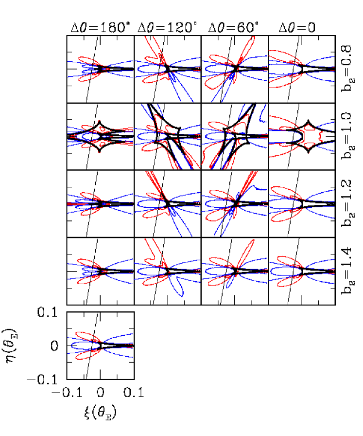
Figure 2: Contours of constant fractional deviation $\delta$ from the single mass lens magnification, as a function of source position $(\xi,\eta)$ in units of the angular Einstein ring, $\theta_{E}$. The parameters of planet 1 are held fixed at $q_{1}=0.003$, $b_{1}=1.2$, while the projected separation $b_{2}$ and the angle between the axes, $\Delta\theta$, are varied for a second planet with $q_{2}=0.001$. The offset panel is the case when only planet 1 is present. Contours are $\delta=\pm 5\%$ (light lines) and $\pm 20\%$ (bold lines). Positive contours are red, negative contours are blue. The caustics ($\delta=\infty$) are shown in black. A trajectory with minimum impact parameter $u_{min}=0.025$ and angle $\theta=260^{\circ}$ with respect to axis 1 is shown.

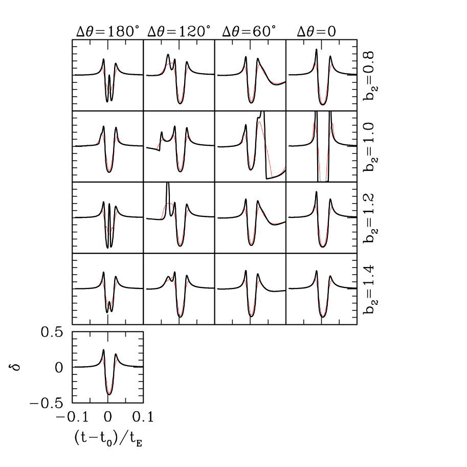
Figure 3: The fractional deviation $\delta$ from a single mass lens as a function of time for the trajectories shown in Fig. 2. The black line is for a source of radius $\rho=0.003$ in units of $\theta_{E}$; the red line is for $\rho=0.01$.

References

- (1)
- (2) Albrow, M., et al. 1996, in IAU Symp. 173, Astrophysical Applications of Gravitational Lensing, C.S. Kochanek & J.N. Hewitt (Dordrecht:Kluwer), 214
- (3)
- (4) Albrow et al. 1997, in Variable Stars and the Astrophysical Returns of Microlensing Surveys, eds. R. Ferlet, J.-P. Maillard, & B. Raban (Gif-sur-Yvette: Editions Frontiéres), 135
- (5)
- (6) Albrow et al. 1998, ApJ, submitted
- (7)
- (8) Alcock, C. et al. 1997a, ApJ, 479, 119
- (9)
- (10) Alcock, C. et al. 1997b, ApJ, 491, 436
- (11)
- (12) Bennett, D. & Rhie, S. H. 1996, ApJ, 472, 660
- (13)
- (14) Butler, P., & Marcy, G. 1996, ApJL, 464, L15
- (15)
- (16) Bolatto, A.D., & Falco, E. E. 1994, ApJ, 436, 112
- (17)
- (18) Di Stefano, R. 1998, ApJ, submitted
- (19)
- (20) Di Stefano, R., & Scalzo, R. 1998a, ApJ, submitted
- (21)
- (22) Di Stefano, R., & Scalzo, R. 1998b, ApJ, submitted
- (23)
- (24) Dominik, M. 1998, in preparation
- (25)
- (26) Gaudi, B. S. 1998, ApJ, submitted
- (27)
- (28) Gaudi, B. S., & Gould, A. 1997, ApJ, 486, 85
- (29)
- (30) Gould, A., & Loeb, A. 1992, ApJ, 396, 104
- (31)
- (32) Griest, K., & Safizadeh, N. 1998, ApJ, submitted (GS)
- (33)
- (34) Lennon, D. J. et al. 1997, The Messenger, in press
- (35)
- (36) Mao, S., & Paczyński, B. 1991, ApJ, 374, 37
- (37)
- (38) Mayor, M., & Queloz, D. 1995, Nature, 378, 355
- (39)
- (40) Paczyński, B. 1996, ARA&A, 34, 419
- (41)
- (42) Peale, S. J. 1997, Icarus, 127, 269
- (43)
- (44) Pratt, M.R. et al. 1996, in IAU Symp. 173, Astrophysical Applications of Gravitational Microlensing, e. C.S. Kochanek & J.N. Hewitt (Dordrecht: Kluwer), 221
- (45)
- (46) Rhie, S.H. 1997, ApJ, 484, 63
- (47)
- (48) Sackett, P.D. 1997, Final Report of the ESO Working Group on the Detection of Extrasolar Planets, astro-ph/9709269
- (49)
- (50) Schneider, P., & Weiss, A. 1986, A&A, 164, 237
- (51)
- (52) Udalski, A., et al. 1994, Acta Astronomica, 44, 227
- (53)
- (54) Wambsganss, J. 1997, MNRAS, 284, 172
- (55)
- (56) Witt, H. 1990, A&A, 236, 311
- (57)