Effect of Correlated Noise on Source Shape Parameters and Weak Lensing Measurements

Abstract

The measurement of shape parameters of sources in astronomical images is usually performed by assuming that the underlying noise is uncorrelated. Spatial noise correlation is however present in practice due to various observational effects and can affect source shape parameters. This effect is particularly important for measurements of weak gravitational lensing, for which the sought image distortions are typically of the order of only 1%. We compute the effect of correlated noise on two-dimensional gaussian fits in full generality. The noise properties are naturally quantified by the noise autocorrelation function (ACF), which is easily measured in practice. We compute the resulting bias on the mean, variance and covariance of the source parameters, and the induced correlation between the shapes of neighboring sources. We show that these biases are of second order in the inverse signal-to-noise ratio of the source, and could thus be overlooked if bright stars are used to monitor systematic distortions. Radio interferometric surveys are particularly prone to this effect because of the long-range pixel correlations produced by the Fourier inversion involved in their image construction. As a concrete application, we consider the search for weak lensing by large-scale structure with the FIRST radio survey. We measure the noise ACF for a FIRST coadded field, and compute the resulting ellipticity correlation function induced by the noise. In comparison with the weak-lensing signal expected in CDM models, the noise correlation effect is important on small angular scales, but is negligible for source separations greater than about $1^{\prime}$. We also discuss how noise correlation can affect weak-lensing studies with optical surveys.

1 Introduction

The measurement of source morphologies in two-dimensional images is a fundamental problem in astronomy. The measurements of shape parameters are usually performed while assuming that the underlying noise is uncorrelated. However, spatial correlation of the noise is always present to some degree, and can significantly affect the derived parameters. In experimental situations, noise correlation can be produced by various effects such as convolution of background light with a beam (or point-spread function), interferometric imaging techniques, CCD readouts, etc.

This effect is particularly important for measurements of weak gravitational lensing. Weak lensing provides a unique opportunity to measure the gravitational potential of massive structures along the line-of-sight (for reviews see Schneider et al. 1992; Narayan & Bartelmann 1996). This technique is now routinely used to map the potential of clusters of galaxies (see Fort & Mellier 1994; Kaiser et al. 1994, for reviews). Detections of the more elusive effect of lensing by large-scale structure have been reported by Villumsen (1995) and Schneider et al. (1997) in small optical fields. The search for a strong detection of the effect on larger angular scales is currently being attempted with present and upcoming wide-field CCDs in the optical band (e.g. Stebbins et al. 1995; Kaiser 1996; Bernardeau et al. 1997), and with the FIRST radio survey (Kamionkowski et al. 1998; Refregier et al. 1998). The main challenge comes from the fact that weak lensing induces image distortions of only about 1%, and thus requires high-precision measurements of source-shape parameters. Correlated noise can produce spurious image distortions and correlations in the shapes of neighboring sources, and therefore must be carefully accounted for in weak lensing studies.

The effect of correlated noise is also particularly important for radio surveys performed with interferometric arrays. In such surveys, images are produced by Fourier inversion of the visibilities from a set of antenna pair. As a result of the incomplete visibility coverage, part of the noise on the image plane contains long range correlations which can extend across an entire field. The effect of these correlations is particularly relevant in the context of recent large radio surveys such as FIRST (Becker et al. 1995; White et al. 1996) and NVSS (Condon et al. 1997). While the present analysis was motivated by our attempt to measure weak lensing by large-scale structure with the FIRST radio survey, most of the following is general and can be applied to any wavelength and imaging technique.

Condon (1997) computed the errors in gaussian fit parameters in the absence of noise correlation. He also gave a semi-quantitative treatment of the noise correlation which relies on simulations. In the present paper, we generalize his approach to include a general analytic treatment of the noise correlation. We show how the spatial correlation of the noise can be naturally characterized by the noise Auto-Correlation Function (ACF). We explicitly derive the effect of noise correlation on source parameters for a general two-dimensional fit and for a two-dimensional gaussian fit. We also consider correlations induced in the parameters of nearby sources. In particular, we focus on the ellipticity correlation functions, which are used in searches for weak lensing by large-scale structure. We apply our formalism to the case of the FIRST radio survey. After measuring the noise ACF for one FIRST coadded field, we compare the noise-induced ellipticity correlations to those expected for weak lensing by large-scale structure. We show that, while they are important on small angular scales, noise correlation effects are negligible for source separations greater than about $1^{\prime}$.

This paper is organized as follows. In §2, we define the noise ACF and show how it can be measured in practice. In §3, we consider a general two-dimensional least-square fit. We derive the bias produced by the noise correlation on the mean, variance and covariance of the fit parameters, and the correlation of the parameters for two neighboring sources. In §4, we apply these results to the case of two-dimensional gaussian fits and compute the error matrix. We explicitly derive the ellipticity correlation function induced by the noise correlation. In §5, we consider the concrete case of the FIRST radio survey. We measure the noise ACF for a FIRST field, compute the induced ellipticity correlation function, and compare the latter to that expected for weak lensing. In §6, we discuss the implications of this effect for optical surveys and related searches for weak lensing by large-scale structure. Finally, §7 summarizes our conclusions.

2 Characterization of the Noise

2.1 Noise Auto-Correlation Function

Let us consider a two-dimensional image with intensity $I({\bf x})$, where ${\bf x}=(x_{1},x_{2})$ is the pixel position. The total intensity can generally be decomposed into

$$I({\bf x})=S({\bf x})+N({\bf x}),$$ (1)

where $S({\bf x})$ is the intensity of detected sources and N(x) is that of the noise. We take the term “noise” to broadly refer to any intensity which is not associated with detected sources. Depending on the context, it can include not only instrumental noise, but also the background light produced by undetected sources.

We assume that, for each pixel, $N({\bf x})$ has mean and variance given by

$$\langle N({\bf x})\rangle \equiv 0{\rm~{}~{}~{}~{}and}$$ (2)

$$\langle N({\bf x})^{2}\rangle \equiv \sigma_{N}^{2},$$ (3)

respectively. The brackets denote an ensemble average which, in practice, is well approximated by a sky average. If necessary, the first equation can be enforced be subtracting a constant term from $N({\bf x})$. The noise is generally correlated from pixel to pixel. This is quantified by the noise ACF which we define as

$$\eta({\bf x}^{ab})\equiv\langle N({\bf x}^{a})N({\bf x}^{b})\rangle,$$ (4)

where ${\bf x}^{ab}\equiv{\bf x}^{b}-{\bf x}^{a}$.

In the case of uncorrelated noise, the noise ACF becomes

$$\eta({\bf x})=\left\{\begin{array}[]{ll}\sigma_{N}^{2},&\mbox{if ${\bf x}=0$}{\rm~{}~{}~{}~{}~{}~{}(uncorrelated)}\\ 0,&\mbox{otherwise}\end{array}\right.$$ (5)

In the continuous limit, i.e. in the limit of small pixel separation $h$, this can be written as

$$\eta({\bf x})\simeq\sigma_{N}^{2}h^{2}\delta^{(2)}({\bf x}),{\rm~{}~{}~{}~{}~{}~{}~{}~{}~{}(uncorrelated)}$$ (6)

where $\delta^{(2)}$ is the two-dimensional Dirac-delta function.

If the noise is gaussian and homogeneous (i.e. statistically invariant under translations), its statistical properties are completely characterized by $\eta({\bf x})$. Generally, however, the noise is non-gaussian, and higher correlation functions are required for a full description. Nevertheless, since our analysis only involves the two-point correlation function $\eta({\bf x})$, it is also valid in the non-gaussian case. In addition, the noise is generally not homogeneous. For instance, the sensitivity and beam shape can vary accross the field-of-view and thus cause the noise properties to depend on position. In this analysis, we assume that this effect is small and that $\eta({\bf x})$ provides an adequate characterization of the noise, at least in an average sense.

2.2 Practical measurement of the noise auto-correlation function

The noise ACF, $\eta({\bf x})$ is easily measured in practice. To do so, discrete sources are (iteratively) removed above a given threshold. Then, $\eta({\bf x})$ is measured by computing the average of equation (4) over pairs of pixels separated by $\eta({\bf x})$.

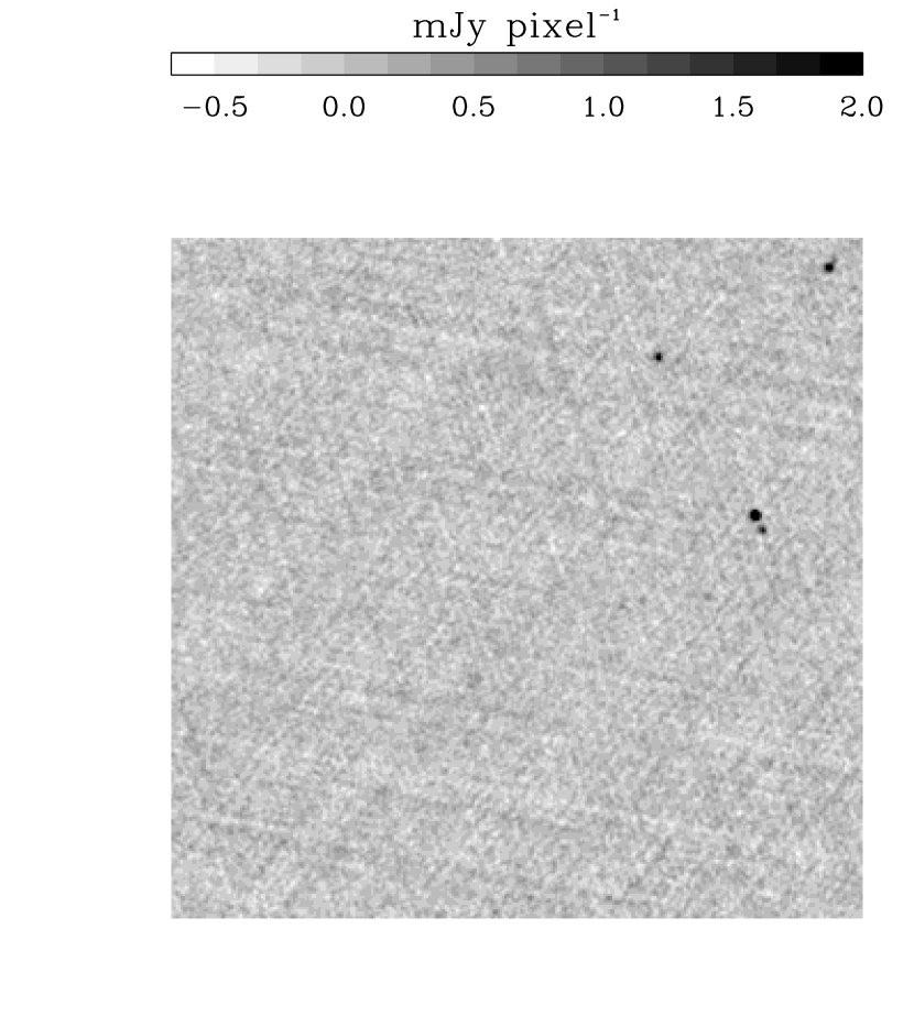
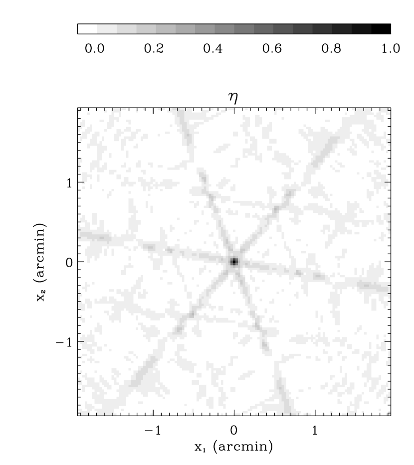
Figure 1 shows a portion of a field in the FIRST radio survey. The contrast was enhanced to make the noise more apparent. Stripe-like patterns in the noise are clearly visible and indicate that the noise is correlated. Figure 2 shows our measurement of the noise ACF for this field. Sources were iteratively removed by excising pixels with intensities above $4\sigma$, and by also removing an area $5.4^{\prime\prime}$ (1 beam width) in radius surrounding each pixel. The measurement of $\eta({\bf x})$ was then performed by randomly choosing pairs of pixels with separations equal to ${\bf x}$. The long range correlations reminiscent of the VLA antenna pattern are apparent. In §5, we discuss the case of the FIRST survey in detail.

Figure 1: Noise patterns for the coadded field 07210+29486E in the FIRST survey. A $9^{\prime}\times 9^{\prime}$ region in the $46.5^{\prime}\times 34.5^{\prime}$ of field is shown. The contrast for the noise was enhanced by clipping pixels with intensities higher than 2 mJy beam^-1. The residual rms intensity is $\sigma_{N}\simeq.15$ mJy beam^-1, for pixels at least 5.4^′′ away from pixels with intensities greater than 0.6 mJy beam^-1. Apart from bright sources, “stripes” in the noise are clearly apparent.

Figure 2: Normalized noise auto-correlation function measured for the coadded field 07210+29486E in the FIRST radio survey. For clarity, only the inner $2^{\prime}\times 2^{\prime}$ arcmin region is shown. The correlation function was normalized to 1 at ${\bf x}=0$. For this field, $\eta(0)\equiv\sigma_{N}^{2}\simeq 2.08\times 10^{-8}$ mJy² beam^-2. For this measurement, the SNR for $\eta(0)$ is 60.

It is easy to show that, in the absence of correlation, the standard deviation, $\sigma[\eta({\bf x})]$, of the measured ACF is

$$\sigma[\eta({\bf x})]=\sigma_{N}^{2}/\sqrt{N_{pairs}({\bf x})},$$ (7)

where $N_{pairs}({\bf x})$ is the number of pixel pairs with separation ${\bf x}$. This provides a measure of the signal-to-noise ratio (SNR) of the ACF measurement, namely

$${\rm SNR}[\eta({\bf x})]\equiv\eta({\bf x})/\sigma[\eta({\bf x})]=\frac{\eta({\bf x})}{\eta(0)}\sqrt{N_{pairs}({\bf x})}.$$ (8)

In the case of figure 2, the number of pairs was chosen to be $N_{pairs}=3600$ for all ${\bf x}$. As a result, the SNR for $\eta(0)$ is 60. This high value of the SNR was achieved owing to the large number of pixels in the FIRST field.

2.3 Noise Correlation from Beam Convolution

As Condon (1997) remarked, a natural example of noise correlation arises when part of the noise is convolved with a beam or Point-Spread Function (PSF). The total noise is then a sum of a convolved component (e.g. background light which gets smoothed by the PSF) and an unconvolved component (e.g. Poisson noise from the detector). For simplicity, we ignore the latter component and suppose that the totality of the noise is convolved as

$$N({\bf x})=\int d^{2}x^{\prime}B({\bf x}-{\bf x}^{\prime})\hat{N}({\bf x}^{\prime}),$$ (9)

where $\hat{N}({\bf x})$ is the intrinsic noise which is assumed to be uncorrelated. The convolution beam $B({\bf x})$ is assumed to be normalized as $\int d^{2}xB({\bf x})\equiv 1$.

As is easy to show using equation (4) and equation (6) for $\hat{N}$, the resulting noise ACF is then

$$\eta({\bf x})=\sigma_{N}^{2}\beta({\bf x}),$$ (10)

with

$$\beta({\bf x}^{ab})\equiv h^{2}\int d^{2}xB({\bf x}-{\bf x}^{a})B({\bf x}-{\bf x}^{b}),$$ (11)

where, again, ${\bf x}^{ab}={\bf x}^{b}-{\bf x}^{a}$. The function $\beta({\bf x})$ can be thought of as the beam ACF.

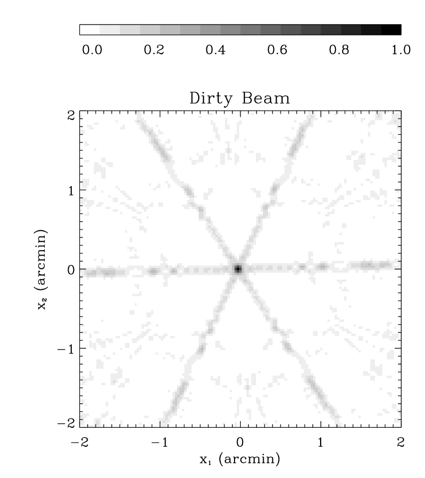
Figure 3 shows the dirty beam for a typical FIRST grid pointing. (The dirty beam is the image of a point source placed at the center of the field prior to CLEANing; see discussion in §5). The coadded field of figure 1 is a weighted sum of 13 similar grid pointings, and therefore does not have a well defined dirty beam. It is nevertheless instructive to compare the noise correlation function of figure 2 to this dirty beam. Qualitatively, the resemblance is striking and reveals that most of the noise is effectively convolved with the dirty beam.

Figure 3: Typical dirty beam for a grid pointing in the FIRST survey. This particular beam was derived using AIPS for the grid pointing 07000+50218 and was normalized to 1 at ${\bf\theta}=0$. This pattern is typical of VLA snapshot images in which limited coverage of the u-v plane is reflected in relatively intense sidelobes along the projected arms of the VLA.

3 General Fit with Correlated Noise

There exist several methods for measuring the shape parameters of sources. The first method consists in fitting a model (usually a gaussian) to the two-dimensional source profile. Another possibility is to measure the multipole moments of the source. The latter method is usually implemented using various window functions to ensure proper convergence (e.g. Schneider & Seitz 1995; Kaiser et al. 1995). The first method is more common in radio interferometric imaging (e.g. AIPS software package; see http://www.cv.nrao.edu/aips/), while the second is usually used with optical images (e.g. FOCAS, SExtractor packages; see Jarvis & Tyson 1981; Bertin & Arnouts 1996, respectively)

Here, we only consider the effect of correlated noise on model fitting. An extension of our results to the multipole moment method is, however, straightforward. In §3.1, we derive the parameter corrections from the noise correlation for the case of a general two-dimensional $\chi^{2}$-fit. We include corrections up to second order in the inverse SNR of the source. In §3.2, we then compute the resulting bias in the mean (§3.2), variance, and covariance of the parameters (§3.3). In §3.4, we compute the induced correlation in the parameters of pairs of neighboring sources. Finally, in §3.5, we consider general functions of the parameters. This analysis builds on the results of Condon (1997) to include an analytical treatment of the noise correlation.

3.1 Least Square Fit

Let us consider a sector of an image consisting of a single source superimposed on noise. We then consider a fit to the two-dimensional source profile with a function $F({\bf x};{\bf a})$, where ${\bf a}=(a_{1},a_{2},...)$ is a vector of parameters. In §4, we will consider the case where $F({\bf x};{\bf a})$ is a two dimensional gaussian with ${\bf a}$ consisting of the gaussian normalization, peak location, and size parameters (see Eq. [51]).

We assume that the fit is “good”, i.e., that the source profile $S({\bf x})$ is well described by

$$S({\bf x})\simeq F({\bf x};\hat{\bf a}),$$ (12)

where $\hat{\bf a}$ is the parameter vector that would be measured in an ideal measurement without noise. The total image intensity (Eq. [1]) thus becomes

$$I({\bf x})=F({\bf x};\hat{\bf a})+N({\bf x}).$$ (13)

We assume that the fit is performed using the method of least squares, without accounting for the noise correlation. This is usually the case for most fitting routines (e.g. AIPS). In other words, the fit is performed by computing the usual functional

$$\chi^{2}({\bf a})=\sum_{p}\frac{\left[I({\bf x}^{p})-F({\bf x}^{p};{\bf a})\right]^{2}}{\sigma_{N}^{2}},$$ (14)

where the sum runs over all the pixels in the image and ${\bf x}^{p}$ are the position of the pixel centers. The best fit parameters ${\bf a}$ are found by minimizing $\chi^{2}({\bf a})$. This minimum occurs when $\frac{\partial\chi^{2}}{\partial a_{l}}({\bf a})=0$, that is, for the value of ${\bf a}$ which satisfies

$$\sum_{p}\left[F({\bf x}^{p};\hat{\bf a})-F({\bf x}^{p};{\bf a})+N({\bf x}^{p})\right]\frac{\partial F}{\partial a_{l}}({\bf x}^{p};\hat{\bf a})=0.$$ (15)

In the noiseless limit ($N\rightarrow 0$), an obvious, if expected, solution is ${\bf a}=\hat{\bf a}$. Note that in the most general case, there could exist more solutions if the system of equation is degenerate. We will not consider this complication here and assume that this solution is unique.

In the presence of noise, the solution ${\bf a}$ will deviate from $\hat{\bf a}$. In most cases, the integrated source flux is much larger than the integrated flux of the noise. This is quantified by the source signal-to-noise ratio, SNR_s which we take to be much larger than 1. We can thus treat the noise $N({\bf x}^{p})$ as a perturbation in equation (15). For this purpose, we rewrite $N({\bf x})$ as $\alpha N({\bf x})$, where $\alpha$ is a dimensionless parameter of the order of $\alpha\sim{\rm SNR}_{s}^{-1}$. We then expand the parameter vector in powers of $\alpha$ as ${\bf a}=\hat{\bf a}+\alpha{\bf a}^{(1)}+\alpha^{2}{\bf a}^{(2)}+O(\alpha^{3})$.

After inserting these expansions in equation (15), Taylor expanding, collecting terms in powers of $\alpha$, and setting $\alpha=1$, we obtain

$$a_{i}=\hat{a}_{i}+D_{il}P_{l}+C_{imn}P_{m}P_{n}+E_{ilkm}P_{m}Q_{lk}+O({\rm SNR}_{s}^{-3}),$$ (16)

where

$$D_{ij} = (H^{-1})_{ij},$$ (17)

$$H_{ij} = \sum_{p}\frac{\partial F}{\partial a_{i}}({\bf x}^{p};\hat{\bf a})\frac{\partial F}{\partial a_{j}}({\bf x}^{p};\hat{\bf a}),$$ (18)

$$B_{ijk} = \sum_{p}\frac{\partial F}{\partial a_{i}}({\bf x}^{p};\hat{\bf a})\frac{\partial^{2}F}{\partial a_{j}\partial a_{k}}({\bf x}^{p};\hat{\bf a}),$$ (19)

$$C_{imn} = -\left[B_{k,rj}+\frac{1}{2}B_{r,kj}\right]D_{ir}D_{km}D_{jn},$$ (20)

$$E_{ilkm} = D_{il}D_{km},$$ (21)

$$P_{i} = \sum_{p}\frac{\partial F}{\partial a_{i}}({\bf x}^{p};\hat{\bf a})N({\bf x}^{p}),{\rm~{}~{}~{}~{}~{}~{}and}$$ (22)

$$Q_{ij} = \sum_{p}\frac{\partial^{2}F}{\partial a_{i}\partial a_{j}}({\bf x}^{p};\hat{\bf a})N({\bf x}^{p}).$$ (23)

Unless otherwise specified, the summation convention is assumed throughout this paper. For reasons which will become clear below, the matrix ${\bf D}$ is called the error matrix (see Condon 1997). In the oversampling regime, i.e. when the pixel spacing $h$ is small compared to the source size, the sums above can be turned into integrals using the substitution

$$\sum_{p}\simeq\frac{1}{h^{2}}\int d^{2}x^{p}.$$ (24)

3.2 Bias in Fit Parameters

We first focus on the bias induced on the source parameters by the noise correlation. By taking an ensemble average of equation (16), we find the mean of the parameter $a_{i}$ to be

$$\left\langle a_{i}\right\rangle=\hat{a}_{i}+D_{il}\left\langle P_{l}\right\rangle+C_{imn}\left\langle P_{m}P_{n}\right\rangle+E_{ilkm}\left\langle P_{m}Q_{lk}\right\rangle+O({\rm SNR}_{s}^{-3}).$$ (25)

But from equation (2), we see that $\left\langle P_{l}\right\rangle=0$ so that the first order term vanishes. Using the definition of $\eta({\bf x})$ (Eq. [4]) we thus find

$$\left\langle a_{i}\right\rangle=\hat{a}_{i}+C_{imn}V_{mn}(0)+E_{ilkm}U_{mlk}(0)+O({\rm SNR}_{s}^{-3}),$$ (26)

where

$$V_{ij}(0) \equiv \sum_{p}\sum_{q}\frac{\partial F}{\partial a_{i}}({\bf x}^{p};\hat{\bf a})\frac{\partial F}{\partial a_{j}}({\bf x}^{q};\hat{\bf a})\eta({\bf x}^{pq}),{\rm~{}~{}~{}~{}and}$$ (27)

$$U_{ijk}(0) \equiv \sum_{p}\sum_{q}\frac{\partial F}{\partial a_{i}}({\bf x}^{p};\hat{\bf a})\frac{\partial^{2}F}{\partial a_{j}\partial a_{k}}({\bf x}^{q};\hat{\bf a})\eta({\bf x}^{pq}).$$ (28)

The operand “$(0)$” was added for future convenience. In the matrices ${\bf V}$ and ${\bf U}$, the noise ACF $\eta({\bf x})$ is averaged over the pixel pairs weighted by parameter derivatives of the source profile. The noise correlation therefore produces a bias in the fit parameters of the order of SNR${}_{s}^{-2}$.

Note however, that this bias does not entirely disappear in the event of uncorrelated noise. Inserting equation (5) in the previous equations, we find that, for uncorrelated noise

$$V_{ij}(0) = \sigma_{N}^{2}H_{ij}{\rm~{}~{}~{}~{}~{}(uncorrelated)},$$ (29)

$$U_{ijk}(0) = \sigma_{N}^{2}B_{ijk}{\rm~{}~{}~{}~{}(uncorrelated)}.$$ (30)

Thus, the ensemble averaged parameter becomes

$$\left\langle a_{i}\right\rangle=\hat{a}_{i}-\frac{1}{2}\sigma_{N}^{2}B_{lkj}D_{li}D_{kj}+O({\rm SNR}_{s}^{-3}){\rm~{}~{}~{}~{}(uncorrelated)}.$$ (31)

Therefore, even for uncorrelated noise, the $\chi^{2}$-fit parameters are biased to second order in SNR_s. This is not surprising: while the $\chi^{2}$-fit is always unbiased if $F({\bf x};{\bf a})$ is linear in ${\bf a}$ (see e.g. Lupton 1993), no such guarantee exist if it is non-linear. It is easy to check that $\left\langle a_{i}\right\rangle$ is indeed unbiased in the linear case. However, most two-dimensional source models, including the gaussian model, are non-linear in their parameters. The correlation in the noise then makes this bias generally more pronounced.

3.3 Parameter Variance and Covariance

We can also compute the covariance of the fit parameters

$${\rm cov}[a_{i},a_{j}]\equiv\left\langle(a_{i}-\left\langle a_{i}\right\rangle)(a_{j}-\left\langle a_{j}\right\rangle)\right\rangle.$$ (32)

Inserting equation (16) in this definition, we obtain

$${\rm cov}[a_{i},a_{j}]=D_{il}D_{jk}V_{lk}(0)+O({\rm SNR}_{s}^{-3}).$$ (33)

In particular, the diagonal elements yield the variance (or squared error) of each of the fit parameters taken separately

$$\sigma^{2}[a_{i}]=D_{il}D_{ik}V_{lk}(0)+O({\rm SNR}_{s}^{-3}),$$ (34)

where the index $i$ is not to be summed over on the right hand side.

In the case of uncorrelated noise, the covariance reduces to

$${\rm cov}[a_{i},a_{j}]=\sigma_{N}^{2}D_{ij}+O({\rm SNR}_{s}^{-3}){\rm~{}~{}~{}~{}~{}(uncorrelated)},$$ (35)

in agreement with Condon (1997), and thereby justifying the term “error matrix” applied to ${\bf D}$. The variance obviously becomes

$$\sigma^{2}[a_{i}]=\sigma_{N}^{2}D_{ii}+O({\rm SNR}_{s}^{-3}){\rm~{}~{}~{}~{}~{}~{}~{}~{}(uncorrelated)},$$ (36)

where, again, the index $i$ is not to be summed over.

3.4 Parameter Correlation Function

Let us now consider two distinct sources, $S^{1}$ and $S^{2}$, in a single field. We assume that the sources are sufficiently distant from each other that the intensity of one source is negligible at the position of the other. If the noise in the field is uncorrelated, the parameter fit to each of the sources would thus be independent. But if the noise is spatially correlated, the parameters of the two sources will be correlated. This effect is particularly relevant for weak lensing studies in which one searches for pairwise correlations in the ellipticities of sources.

To quantify the effect, we define the parameter correlation function as

$$w^{aa}_{ij}(\hat{\bf x}^{12})=\left\langle(a^{1}_{i}-\left\langle a^{1}_{i}\right\rangle)(a^{2}_{j}-\left\langle a^{2}_{j}\right\rangle)\right\rangle,$$ (37)

where ${\bf a}^{r}$ is the fit-parameter vector for source $S^{r}$, and $\hat{\bf x}^{12}$ is the separation between the (noiseless) source centroids.

Inserting equation (16) into this definition yields

$$w^{aa}_{ij}(\hat{\bf x}^{12})=D_{il}^{1}D_{jk}^{2}V_{lk}^{12}(\hat{\bf x}^{12})+O({\rm SNR}_{s}^{-3}),$$ (38)

where,

$$D_{ij}^{r}\equiv\sum_{p}\frac{\partial F}{\partial a_{i}}({\bf x}^{p};\hat{\bf a}^{r})\frac{\partial F}{\partial a_{j}}({\bf x}^{p};\hat{\bf a}^{r}),$$ (39)

and

$$V_{ij}^{12}(\hat{\bf x}^{12})=\sum_{p}\sum_{q}\frac{\partial F}{\partial a_{i}}({\bf x}^{p};\hat{\bf a}^{1})\frac{\partial F}{\partial a_{j}}({\bf x}^{q};\hat{\bf a}^{2})\eta({\bf x}^{pq}).$$ (40)

The fit-parameter correlation is therefore of order SNR^-2.

In the absence of noise correlation (Eq. [5]), $V_{ij}^{12}(\hat{\bf x}^{12})$ becomes

$$V_{ij}^{12}(\hat{\bf x}^{12})=\sigma_{N}^{2}\sum_{p}\frac{\partial F}{\partial a_{i}}({\bf x}^{p};\hat{\bf a}^{1})\frac{\partial F}{\partial a_{j}}({\bf x}^{q};\hat{\bf a}^{2}).$$ (41)

As is the case for a gaussian fitting function, the parametric partial derivatives, $\frac{\partial F}{\partial a_{i}}$, are often spatially localized. In this case, the above sum vanishes, if the sources are sufficiently distant from each other. Thus, for $|\hat{\bf x}|$ much larger than the source sizes, and for well-behaved fitting functions

$$w^{aa}_{ij}(\hat{\bf x})\simeq 0{\rm~{}~{}~{}~{}(uncorrelated)}.$$ (42)

As expected, the fit parameters of the two sources are then uncorrelated if the noise is itself spatially uncorrelated.

3.5 Functions of the Parameters

We can also compute the effect of correlated noise on functions of the parameters. Let us consider a set of such functions, $t_{i}({\bf a})$. In §4.3, we will consider an application were the $t_{i}$’s are the 2 components of the ellipticity of the source. In the presence of noise, the value of the functions are perturbed as (see Eq. [16])

$$t_{i}({\bf a})=t_{i}(\hat{\bf a})+\frac{\partial t_{i}}{\partial a_{j}}(\hat{\bf a})D_{jk}P_{k}+O({\rm SNR}_{s}^{-2}).$$ (43)

The covariance of the $t_{i}$’s is thus

$${\rm cov}[t_{i},t_{j}] \equiv \left\langle\left(t_{i}-\left\langle t_{i}\right\rangle\right)\left(t_{j}-\left\langle t_{j}\right\rangle\right)\right\rangle$$ (44)

$$= K_{ik}K_{jl}V_{kl}(0)+O({\rm SNR}_{s}^{-3}).$$

where we have defined

$$K_{ij}\equiv\frac{\partial t_{i}}{\partial a_{k}}(\hat{\bf a})D_{kj}.$$ (45)

In the absence of noise correlation (Eq. [29]), this covariance matrix becomes

$${\rm cov}[t_{i},t_{j}]=\sigma_{N}^{2}\frac{\partial t_{i}}{\partial a_{k}}(\hat{\bf a})\frac{\partial t_{j}}{\partial a_{l}}(\hat{\bf a})D_{kl}+O({\rm SNR}_{s}^{-3}),{\rm~{}~{}~{}~{}~{}~{}(uncorrelated)}$$ (46)

in accordance with Condon (1997).

For a pair of two distinct sources, $S^{1}$ and $S^{2}$, the correlation function for the $t_{i}$’s is easily found to be

$$w^{tt}_{ij}(\hat{\bf x}^{12}) \equiv \left\langle\left(t_{i}({\bf a}^{1})-\left\langle t_{i}({\bf a}^{1})\right\rangle\right)\left(t_{j}({\bf a}^{2})-\left\langle t_{j}({\bf a}^{2})\right\rangle\right)\right\rangle$$ (47)

$$= K_{ik}^{1}K_{jl}^{2}V_{kl}^{12}(\hat{\bf x}^{12})+O({\rm SNR}_{s}^{-3}).$$

where

$$K_{ij}^{r}\equiv\frac{\partial t_{i}}{\partial a_{k}}(\hat{\bf a}^{r})D_{kj}^{r}.$$ (48)

In the absence of noise correlation, and for distinct sources with well-behaved fitting functions (Eq. [41]), this correlation function is simply

$$w^{tt}_{ij}(\hat{\bf x})\simeq 0{\rm~{}~{}~{}~{}~{}~{}(uncorrelated)}$$ (49)

4 Gaussian Fit

In the previous section, we derived the bias, covariance, and correlation function of parameters for a general fit in the presence of correlated noise. In this section, we apply these results to the case which is of most practical interest, namely that of a two-dimensional gaussian fit.

4.1 Gaussian Parametrization

As the fitting function $F({\bf x};{\bf a})$, we consider the the following parametrization of a two-dimensional elliptical gaussian

$$G({\bf x},{\bf a})\equiv{\cal A}e^{-\frac{1}{2}({\bf x}-{\bf x}^{a})^{T}{\bf A}({\bf x}-{\bf x}^{a})},$$ (50)

where $\cal A$ is the amplitude, ${\bf x}^{a}$ is the centroid vector, ${\bf A}$ is a symmetric positive-definite $2\times 2$ matrix which defines the shape and orientation of the gaussian, and the superscript ^T denotes the transpose operation. We choose the parameter vector to be

$${\bf a}\equiv(x_{1}^{a},x_{2}^{a},{\cal A},A_{11},A_{12},A_{22}).$$ (51)

Note that this parametrization is different from that of Condon (1997), and was to chosen because it is easier to relate to the parameters used in weak-lensing measurements.

It is convenient to compute the first few multipole moments $G^{(n)}$ of $G$. With the above definition, we find

$$G^{(0)} \equiv \int d^{2}xG({\bf x},{\bf a})=\pi{\cal A}|A|^{-1},$$ (52)

$$\frac{G_{i}^{(1)}}{G^{(0)}} \equiv \frac{1}{G^{(0)}}\int d^{2}xx_{i}G({\bf x},{\bf a})=x_{i}^{a},$$ (53)

$$\frac{G_{ij}^{(2)}}{G^{(0)}} \equiv \frac{1}{G^{(0)}}\int d^{2}x(x_{i}-x_{i}^{a})(x_{j}-x_{j}^{a})G({\bf x},{\bf a})=(A^{-1})_{ij},$$ (54)

where $|A|$ is the determinant of ${\bf A}$. Note that

$${\bf J}\equiv{\bf A}^{-1}=|A|^{-1}\left(\begin{array}[]{cc}A_{22}&-A_{12}\\ -A_{12}&A_{11}\end{array}\right)$$ (55)

is exactly equal to the normalized quadrupole moments of $G$. It can be diagonalized as

$${\bf J}={\bf R}(-\alpha)\left(\begin{array}[]{cc}a^{2}&0\\ 0&b^{2}\end{array}\right){\bf R}(-\alpha)^{T}$$ (56)

where $a$, $b$ are the ($1\sigma$) major and minor axes, and $\alpha$ is the position angle measured counter-clockwise from the positive x-axis. The rotation matrix ${\bf R}$ is defined as

$${\bf R}(\varphi)\equiv\left(\begin{array}[]{cc}\cos\varphi&\sin\varphi\\ -\sin\varphi&\cos\varphi\end{array}\right).$$ (57)

Inverting these relations yields

$$(a^{2},b^{2}) = \frac{1}{2}\left[J_{11}+J_{22}\pm\sqrt{(J_{11}-J_{22})^{2}+4J_{12}^{2}}\right],$$ (58)

$$\tan 2\alpha = \frac{2J_{12}}{J_{11}-J_{22}}.$$ (59)

4.2 Source and Noise Matrices

We are now in a position to compute the source and noise matrices in equations (17-23). For this purpose, we first compute the partial derivatives of $G$. We find,

$$\frac{\partial G}{\partial{\bf a}} = G\left({[(x_{1}-x_{1}^{a})A_{11}+(x_{2}-x_{2}^{a})A_{12}],[(x_{2}-x_{2}^{a})A_{22}+(x_{1}-x_{1}^{a})A_{12}],\cal A}^{-1},\right.$$ (60)

$$\left.-\frac{1}{2}(x_{1}-x_{1}^{a})^{2},-(x_{1}-x_{1}^{a})(x_{2}-x_{2}^{a}),-\frac{1}{2}(x_{2}-x_{2}^{a})^{2}\right)$$

In the continuous limit (Eq. [24]), the components of the matrix ${\bf H}$ (Eq. [18]) have a closed form, i.e.,

$${\bf H}\simeq\frac{\pi{\cal A}^{2}}{h^{2}\sqrt{|A|}}\times$$ (67)

$$\left(\begin{array}[]{cccccc}\frac{1}{2}A_{11}&\frac{1}{2}A_{12}&0&0&0&0\\ \frac{1}{2}A_{12}&\frac{1}{2}A_{22}&0&0&0&0\\ 0&0&{\cal A}^{-2}&-\frac{1}{4}|A|^{-1}{\cal A}^{-1}A_{22}&\frac{1}{2}|A|^{-1}{\cal A}^{-1}A_{12}&-\frac{1}{4}|A|^{-1}{\cal A}^{-1}A_{11}\\ 0&0&-\frac{1}{4}|A|^{-1}{\cal A}^{-1}A_{22}&\frac{3}{16}|A|^{-2}A_{22}^{2}&-\frac{3}{8}|A|^{-2}A_{22}A_{12}&\frac{1}{16}|A|^{-2}A^{2}\\ 0&0&\frac{1}{2}|A|^{-1}{\cal A}^{-1}A_{12}&-\frac{3}{8}|A|^{-2}A_{22}A_{12}&\frac{1}{4}|A|^{-2}A^{2}&-\frac{3}{8}|A|^{-2}A_{11}A_{12}\\ 0&0&-\frac{1}{4}|A|^{-1}{\cal A}^{-1}A_{11}&\frac{1}{16}|A|^{-2}A^{2}&-\frac{3}{8}|A|^{-2}A_{11}A_{12}&\frac{3}{16}|A|^{-2}A_{11}^{2}\end{array}\right),$$

where $A^{2}\equiv(A_{11}A_{22}+2A_{12}^{2})$. Note that the amplitude and shape parameters mix with each other, but not with the position parameters.

By inverting the above matrix, we find the error matrix ${\bf D}$ to be

$${\bf D}\simeq\frac{2h^{2}\sqrt{|A|}}{\pi{\cal A}^{2}}\left(\begin{array}[]{cccccc}|A|^{-1}A_{22}&-|A|^{-1}A_{12}&0&0&0&0\\ -|A|^{-1}A_{12}&|A|^{-1}A_{11}&0&0&0&0\\ 0&0&{\cal A}^{2}&{\cal A}A_{11}&{\cal A}A_{12}&{\cal A}A_{22}\\ 0&0&{\cal A}A_{11}&4A_{11}^{2}&4A_{11}A_{12}&4A_{12}^{2}\\ 0&0&{\cal A}A_{12}&4A_{11}A_{12}&2(A_{11}A_{22}+A{12}^{2})&4A_{12}A_{22}\\ 0&0&{\cal A}A_{22}&4A_{12}^{2}&4A_{22}A_{12}&4A_{22}^{2}\end{array}\right).$$ (68)

The ${\bf B}$ matrix of equation (19) can be computed in a similar way. The calculation for this $6^{3}$ component matrix is however cumbersome. Since it does not enter in the parameter correlation function on which we will now focus, we will not consider it further.

The noise matrices ${\bf P}$ (Eq. [22]) and ${\bf Q}$ (Eq. [23]) can not be computed without knowledge of the noise ACF, $\eta({\bf x})$. In practice, $\eta({\bf x})$ has a complicated ${\bf x}$-dependence. As a result, ${\bf P}$ and ${\bf Q}$ must be computed numerically using the direct measurement of $\eta({\bf x})$, along with the expressions for the derivatives of $G$ (Eq. [60]). In the next section, we study the effect of the noise correlation on the source ellipticity, a combination of the source parameters which is particularly relevant for weak lensing measurements. (By source ellipticity we mean the ellipticity of the observed source image and not the ellipticity in the source plane, as is common in the lensing nomenclature).

4.3 Source Ellipticities

The shear produced by weak gravitational lensing produces distortions in the shapes of background sources. The most direct way to detect this effect is to look for correlations in the ellipticities of sources. Measurements of the ellipticity involve integrals that are more spatially extended than that of the flux and position of a source. Consequently, we expect the ellipticity to be particularly sensitive to the spatial correlation of the noise. Here, we compute the magnitude of this effect on the ellipticities and on the ellipticity correlation function.

A number of ellipticity measures have been used in weak lensing studies (e.g. Schneider 1995; Bonnet & Mellier 1995). Here, we will use the ellipticity measure considered by Miralda-Escudé (1991), Kaiser & Squires (1993) and others, which has the advantage of being easily related to the gaussian parameters of equation (50). In this definition, the ellipticity is defined as a two component “vector” $\epsilon$ whose components are given by

$$\epsilon_{1}=\frac{J_{11}-J_{22}}{J_{11}+J_{22}},~{}~{}~{}~{}~{}~{}\epsilon_{2}=\frac{2J_{12}}{J_{11}+J_{22}}.$$ (69)

This can be rewritten in terms of the major axis, minor axis, and position angle of the source as $\mbox{\boldmath$\epsilon$}=\frac{a^{2}-b^{2}}{a^{2}+b^{2}}(\cos 2\alpha,\sin 2\alpha)$. The component $\epsilon_{1}$, sometimes written as $\epsilon_{+}$, describes stretches along the $x$ and $y$-axes, while $\epsilon_{2}$, sometimes written as $\epsilon_{\times}$, describes stretches at $\pm 45^{\circ}$ with respect to these axes. In a coordinate system $(x_{1}^{\prime},x_{2}^{\prime})$ rotated by $\varphi$ counter-clockwise from the positive $x_{1}$-axis, the components of $\epsilon$ are

$$\epsilon_{i}^{\prime}=R_{ij}(2\varphi)\epsilon_{j},$$ (70)

where ${\bf R}$ is the rotation matrix defined in equation (57). This shows that $\epsilon$ is not a true vector since it has a period of $\pi$ in $\varphi$. (In fact, $\epsilon$ can be written as a symmetric traceless $2\times 2$ tensor).

The ellipticity can be rewritten in terms of the gaussian fit parameters (see Eq. [55]) as

$$\epsilon_{1}=\frac{A_{22}-A_{11}}{A_{11}+A_{22}},~{}~{}~{}~{}\epsilon_{2}=\frac{-2A_{12}}{A_{11}+A_{22}}.$$ (71)

The partial derivative matrix of $\epsilon$ is thus

$$\frac{\partial\mbox{\boldmath$\epsilon$}}{\partial{\bf a}}=2(A_{11}+A_{22})^{-2}\left(\begin{array}[]{cccccc}0&0&0&-A_{22}&0&A_{11}\\ 0&0&0&A_{12}&-(A_{11}+A_{22})&A_{12}\end{array}\right).$$ (72)

Note that the position parameters, $x_{1}^{a}$ and $x_{2}^{a}$, have decoupled from the ellipticity matrices and can thus be dropped. There are kept here for consistency. It is then straightforward to compute the ${\bf K}$ matrix (Eq. [48]). We find

$${\bf K}\simeq-\frac{16h^{2}|A|^{\frac{3}{2}}}{\pi{\cal A}^{2}(A_{11}+A_{22})^{2}}\left(\begin{array}[]{cccccc}0&0&0&A_{11}&0&-A_{22}\\ 0&0&0&A_{12}&\frac{1}{2}(A_{11}+A_{22})&A_{12}\end{array}\right).$$ (73)

With this result and a measurement of the noise ACF $\eta({\bf x})$, the covariance cov$[\epsilon_{i},\epsilon_{j}]$ and correlation function $w_{ij}^{\epsilon\epsilon}({\bf x})$ of the ellipticity are readily calculated using equations (44) and (47).

We now focus on $w_{ij}^{\epsilon\epsilon}({\bf x})$ which is of interest for measurements of weak lensing by large-scale structure. To be explicit, this correlation function is defined as

$$w_{ij}^{\epsilon\epsilon}({\bf x}^{12})\equiv\left\langle\epsilon_{i}^{1}\epsilon_{j}^{2}\right\rangle$$ (74)

In practice, it is usually sufficient to consider the correlation of two sources which are identical and circular. In this simplified case, the unperturbed parameters for source $S^{1}$ and $S^{2}$ are $\hat{\bf a}^{1}=({\cal A},\hat{x}_{1}^{1},\hat{x}_{2}^{1},a^{-2},0,a^{-2})$, and $\hat{\bf a}^{2}=({\cal A},\hat{x}_{1}^{2},\hat{x}_{2}^{2},a^{-2},0,a^{-2})$, where $a$ is the ($1\sigma$) radius of the sources, ${\cal A}$ is their amplitude, and $\hat{x}_{i}^{r}$ gives their (unperturbed) centroid position. In this case, the ellipticity correlation function reduces to

$$w_{ij}^{\epsilon\epsilon}(\hat{x}^{12})\simeq\frac{4h^{4}}{\pi^{2}a^{8}{\cal A}^{2}}\frac{1}{h^{4}}\int d^{2}x^{1}d^{2}x^{2}X_{ij}({\bf x}^{1}-\hat{\bf x}^{1},{\bf x}^{2}-\hat{\bf x}^{2})e^{-\frac{({\bf x}^{1}-\hat{\bf x}^{1})^{2}+({\bf x}^{2}-\hat{\bf x}^{2})^{2}}{2a^{2}}}\eta({\bf x}^{12})+O({\rm SNR}_{s}^{-3}),$$ (75)

where

$${\bf X}(\mbox{\boldmath$\xi$}^{1},\mbox{\boldmath$\xi$}^{2})\equiv\left(\begin{array}[]{cc}[(\xi_{1}^{1})^{2}-(\xi_{2}^{1})^{2}][(\xi_{1}^{2})^{2}-(\xi_{2}^{2})^{2}]&2\xi_{1}^{2}\xi_{2}^{2}[(\xi_{1}^{1})^{2}-(\xi_{2}^{1})^{2}]\\ 2\xi_{1}^{1}\xi_{2}^{1}[(\xi_{1}^{2})^{2}-(\xi_{2}^{2})^{2}]&4\xi_{1}^{1}\xi_{2}^{1}\xi_{1}^{2}\xi_{2}^{2}\end{array}\right).$$ (76)

It is also convenient to consider the ellipticities measured with respect to axes parallel and perpendicular to ${\bf x}^{12}$, the vector connecting two sources ( Kamionkowski et al. 1998). Let us write this vector in polar coordinates as ${\bf x}^{12}=(\theta^{12},\varphi^{12})$, where $\theta^{12}$ is the norm of the vector and $\varphi^{12}$ the angle it substands with the $x_{1}$-axis. From equation (70), the components of the ellipticities rotated into this coordinate system are $\epsilon_{i}^{r}\equiv R_{ij}(2\varphi^{12})\epsilon_{j}$. The correlation function of the rotated ellipticities is then

$$w_{ij}^{rr}(\theta^{12},\varphi^{12})\equiv\left\langle\epsilon_{i}^{r,1}\epsilon_{j}^{r,2}\right\rangle=R_{ik}(2\varphi^{12})R_{jl}(2\varphi^{12})w_{kl}^{\epsilon\epsilon}(\theta^{12},\varphi^{12}).$$ (77)

Following the notation of Kaiser (1992), we identify $w_{11}^{rr}({\bf x})\equiv C_{1}({\bf x})$, and $w_{22}^{rr}({\bf x})\equiv C_{2}({\bf x})$. We can also define a third independent correlation function $w_{12}^{rr}({\bf x})\equiv w_{21}^{rr}({\bf x})\equiv C_{3}({\bf x})$, which should vanish if the noise is invariant under parity conservation.

These correlation functions can then be averaged over $\varphi^{12}$ by defining

$$\bar{w}_{ij}^{rr}(\theta)\equiv\frac{1}{\pi}\int_{0}^{\pi}d\varphi w_{ij}^{rr}(\theta,\varphi).$$ (78)

In the above notation, we simply write the azimuthally averaged correlation functions as $\bar{w}_{11}^{rr}(\theta)\equiv C_{1}(\theta)$, $\bar{w}_{22}^{rr}(\theta)\equiv C_{2}(\theta)$ and $\bar{w}_{12}^{rr}(\theta)\equiv\bar{w}_{21}^{rr}(\theta)\equiv C_{3}(\theta)$. In the context of weak lensing studies, $C_{1}(\theta)$ and $C_{2}(\theta)$ can be directly related to the power spectrum of density perturbations along the line of sight (see e.g. Kaiser 1992).

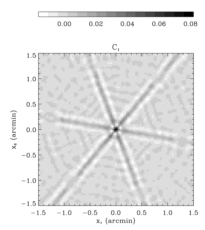
Figure 4 shows the rotated correlation functions for the FIRST coadded field of figures 1 and 2. A source size of $a=2.45^{\prime\prime}$ and signal-to-noise ratio of SNR${}_{s}=5$ were chosen. Figures 7, 8, and 9 show the corresponding azimuthally averaged correlation functions. In the next section, we will describe these results in detail and discuss their implications for weak lensing measurements.

Figure 4: Ellipticity correlation functions for the coadded field 07210+29486E. Each correlation function $C_{1}$, $C_{2}$ and $C_{3}$ is plotted as a function of the separation vector ${\bf x}$ in panels a, b, and c, respectively. For each source pair member, source signal-to-noise ratio was set to SNR${}_{s}=5$, while the $1\sigma$ source size was set to $a=2.45^{\prime\prime}$. This corresponds to FWHM convolved and deconvolved diameters of $5.76^{\prime\prime}$ and $2^{\prime\prime}$, respectively. The clean beam for the FIRST survey has a FWHM diameter of $5.4^{\prime\prime}$.

Figure 4b: [See caption above]

Figure 4c: [See caption above]

5 Application to the FIRST Radio Survey

In this section, we apply the general formalism developed above to the specific case of the FIRST radio survey (Becker et al. 1995; White et al. 1996). The current version of the FIRST survey contains about $4\times 10^{5}$ sources, and covers about $4.3\times 10^{3}$ square degrees. The survey fields were observed at 1.4 GHz with the VLA in the B configuration. The $5\sigma$ detection limit of the survey is about 0.75 mJy. The pixel size for the survey maps is 1.8^′′, while the restoring beam is 5.4^′′ (FWHM). The restoring beam is thus reasonably well sampled. This allows us to take the continuous limit (Eq. [24]) in our calculation. In addition, the relatively high angular resolution allows an accurate measurement of source morphologies. We are in the process of attempting to detect the effect of weak lensing by large-scale structure with this unique database (Kamionkowski et al. 1998; Refregier et al. 1998).

Because of the observing time limitations for a survey of this magnitude, the observations had to be performed in the snapshot mode with integration times of 5 seconds. The interferometric data (or “UV” data) for each snapshot pointing was then Fourier transformed to construct a “dirty” image. The resulting pointing images were CLEANed using algorithms adapted from the standard AIPS deconvolution package. The final survey fields were produced by a weighted sum of the grid pointing images. At a given point, approximately 12 pointings contribute to the coadded field. Sources were then detected and their shape parameters measured, using a two-dimensional gaussian fit.

Even though the grid pointing strategy was designed to optimize the signal-to-noise ratio of the coadded images, the final maps still suffer from the limited UV-coverage of the snapshot pointings. As a result, typical coadded maps contain small but noticeable “stripes” in the noise (see figure 1). In other words, the noise is correlated. As we discussed above, this affects the source parameters derived by the fitting routine. In particular, the effect of correlated noise is a potential systematic effect in a search for correlations in the source ellipticities produced by weak lensing.

5.1 Noise Auto-Correlation Function

As a specific case, we considered the coadded field 07210+29486E in the FIRST survey. This field covers a solid angle of $46.5^{\prime}\times 34.5^{\prime}$, with a pixel size of 1.8^′′. Figure 1 shows a portion of this field with the contrast enhanced to make the noise more apparent. Bright radio sources are apparent in the right hand corner. In addition, the stripe-like nature of the noise is visible. For this analysis, pixels with intensities above .6 mJy beam^-1 (corresponding to about $4\sigma$) were excised from the field. The excised regions were then padded by 5.4^′′ to avoid contamination of the noise by the source side wings. The residual noise has a standard deviation of $\sigma_{N}\simeq.15$ mJy beam^-1. (Intensities are quoted in mJy beam^-1, were the beam refers to the restoring beam with a FWHM diameter of 5.4^′′.) The median noise standard deviation for the FIRST survey is 0.14 mJy beam^-1, with 95% of the FIRST area having a noise standard deviation less than 0.17 mJy beam^-1 (White et al. 1996). This makes the coadded field 07210+29486E somewhat noisy, yet representative of the FIRST survey.

Figure 2 shows our measurement of the noise ACF, $\eta({\bf x})$, for this field. For this measurement, the SNR for $\eta(0)$ is 60 (see Eq. [8]). For convenience, $\eta({\bf x})$ was normalized to 1 at ${\bf x}=0$ in this figure. In addition to a prominent central peak, the ACF shows marked radial structures. These structures are reminiscent of the VLA antenna pattern and characterize the “stripes” which are visible in the noise.

Each grid pointing is characterized by a dirty beam. (It is the Fourier transform of the UV coverage and is equal to the dirty image produced by a point source at the phase tracking center). In general, the dirty beam shape varies from one grid pointing to another due to differing geometries, flagged antennas, etc. As a result, coadded fields, which are composed of several grid pointings, do not have a well defined dirty beam. It is nevertheless instructive to qualitatively compare our measurement of the noise ACF with a typical grid pointing dirty beam. Figure 3 shows such a dirty beam for the grid pointing 07000+50218. The qualitative resemblance with $\eta({\bf x})$ is striking. This shows that a large fraction of the noise is effectively convolved with the dirty beam.

5.2 Ellipticity Correlation Functions

Of practical interest for weak lensing measurements, is the effect of the correlated noise on the ellipticity correlation functions. Figure 4 shows the rotated correlation functions $C_{1}({\bf x})$, $C_{2}({\bf x})$ and $C_{3}({\bf x})$ (Eq [77]) for the coadded field of figure 1. A source size of $a=2.45^{\prime\prime}$ was chosen. This corresponds to a FWHM diameter of $5.76^{\prime\prime}$, that is to a deconvolved FWHM diameter of $2^{\prime\prime}$, for a restoring beam of $5.4^{\prime\prime}$. The source signal-to-noise ratio was set to SNR${}_{s}=5$. These parameters correspond to both the detection and resolution limit of the FIRST survey and can thus be considered as “worse-case” parameters for a weak lensing search.

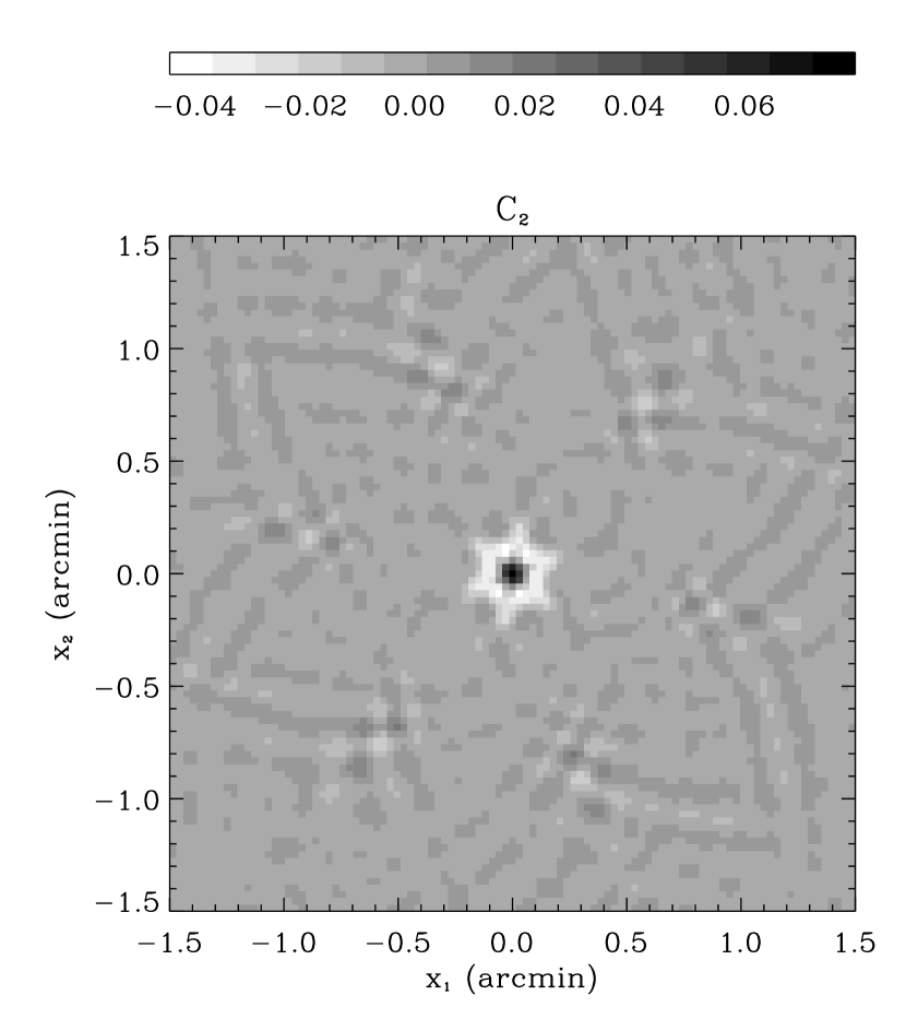
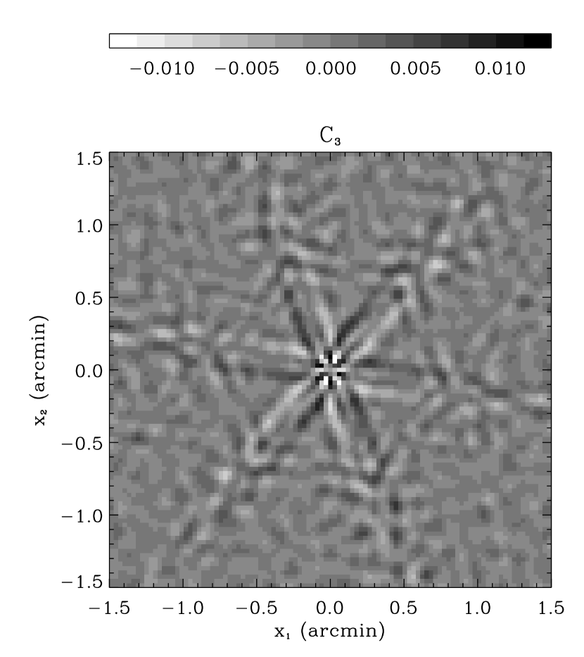
The symmetric patterns of $\eta({\bf x})$ (figure 2) are also clearly apparent on figure 4. However, the patterns are different for each of the correlation functions. The first correlation function, $C_{1}({\bf x})$ exhibits a pronounced star-like pattern with radial elongation on each arm. On the other hand, $C_{2}({\bf x})$ is mostly characterized by a negative correlation close to the center. Finally, $C_{3}({\bf x})$ exhibits star-like patterns but of much smaller amplitude than that of $C_{1}({\bf x})$ and $C_{3}({\bf x})$. The last fact is expected for a non-parity violating noise pattern.

Figure 7 shows the azimuthally averaged correlation functions, $C_{1}(\theta)$, $C_{2}(\theta)$ and $C_{3}(\theta)$ as a function of $\theta$. These are simply the radial profiles of the rotated correlation functions of figure 4. They were derived by Monte-Carlo averaging over $4\times 10^{5}$ separation vectors ${\bf x}$ picked randomly within a radius of $50^{\prime}$. The thick lines correspond to a source size of $a=2.45^{\prime\prime}$, while the thin lines corresponds to $a=3.40^{\prime\prime}$. In both cases, the source signal-to-noise ratio was set to SNR${}_{s}=5$, as before. For $\theta\lesssim 0.4^{\prime}$, $C_{1}(\theta)$ is positive while $C_{2}(\theta)$ is negative and drops off faster. Note that both $C_{1}(\theta)$ and $C_{2}(\theta)$ are significantly non-zero well beyond the source radius $a$. This is of course due to the long-range features in $\eta({\bf x})$ (figure 2). At all angles, $C_{3}(\theta)$ remains smaller and oscillates around 0. As we remarked above, this is expected for non-parity violating noise.

Figure 7: Azimuthally-averaged ellipticity correlation functions for the same coadded field. Each correlation functions, $C_{1}$, $C_{2}$, and $C_{3}$, are plotted as a function of the separation radius $\theta$. A source signal-to-noise ratio of SNR${}_{s}=5$ was assumed. The correlation functions scale as $C_{i}\propto{\rm SNR}_{s}^{-2}$. The correlation functions are plotted for a source size of $a=2.45^{\prime\prime}$ (thick lines) and of $a=3.40^{\prime\prime}$ (thin lines).

A comparison between the thick and thin lines in figure 7 shows how the ellipticity correlation functions depend on the source size. For larger source sizes, $C_{1}(\theta)$ and $C_{2}(\theta)$ keep the same qualitative behavior but have a lower maximum amplitude and drop off more slowly. This is expected since larger source sizes effectively smooth out the sharp features in the noise ACF (figure 2; see Eq. [75]).

Figure 8 shows the long range behavior of the ellipticity correlation functions. For angles larger than $\theta=10^{\prime}$, a mosaic of 4 fields contiguous with 07210+29486E was used to compute the noise ACF $\eta({\bf x})$. The error bars shown for $C_{1}(\theta)$ are the error in the mean derived from the Monte-Carlo sampling described above. Since the separation plane was undersampled, these error bars provide a good estimate of the uncertainty in the correlation functions. As is apparent on this figure, all three correlation functions are consistent with 0 for $\theta\gtrsim 1^{\prime}$.

Figure 8: Same as the previous figure but this time focusing on the large-angle behavior of the correlation functions. The correlation functions are only plotted for a source size of $a=2.45^{\prime\prime}$. The error bars are the $1\sigma$ errors in the mean derived from the Monte-Carlo integration. For clarity, they were only shown for $C_{1}(\theta)$. The correlation functions are all consistent with 0 for $\theta\gtrsim 1^{\prime}$.

5.3 Consequences for Weak Lensing Searches

As was demonstrated above, correlated noise affects the ellipticity correlation functions in the FIRST survey. We now compare the amplitude of this systematic effect with the signal expected for weak lensing by large-scale structure.

Figure 9 shows the noise-induced correlation functions, $C_{1}(\theta)$ and $C_{2}(\theta)$ on a log-log scale. The absolute value of the correlation functions are plotted, with positive and negative values indicated by squares and stars, respectively. For comparison, the (absolute value of the) correlation functions expected for weak lensing in CDM models are also displayed. The four models correspond to the COBE-normalized CDM models in table 2 and figure 4 in Kamionkowski et al. (1998). Models 1-3 correspond to a standard, tilted, and lambda CDM model, respectively. Model 4 corresponds to a standard CDM model with a smaller Hubble constant than that of Model 1. In all models, only linear evolution of density perturbations were considered.

Figure 9: Comparison with the weak lensing correlation functions expected in CDM models. The smooth curves show the ellipticity correlation functions for the four COBE-normalized CDM models of Kamionkowski et al. (1998). The top and bottom curves for each model correspond to $C_{1}$ and $C_{2}$, respectively. The broken lines correspond to the ellipticity correlation functions induced by the noise correlation, for sources with $a=2.45^{\prime\prime}$ and SNR${}_{s}=5$. In all cases, the absolute value of the correlation function is shown. To preserve a sense of the noisy behavior of the noise-induced correlation functions, positive and negative values are indicated by squares and stars, respectively.

As we noted above, noise correlation produces significant biases in $C_{1}(\theta)$ and $C_{2}(\theta)$ for $\theta\lesssim 1^{\prime}$. In this angular range, the noise-induced correlation functions exceed those expected for weak lensing for all models. (The inclusion of nonlinear evolution of density perturbations increases the estimates of the weak lensing signal for $\theta\lesssim 10^{\prime}$ by only a factor of a few and therefore does not significantly alter this conclusion; see Jain & Seljak 1997.)

For angles $\theta\gtrsim 1^{\prime}$, we showed above that the noise-induced correlation functions are consistent with zero, within the Monte-Carlo uncertainties. This can be seen by the alternation of squares and stars in figure 9. The noise-induced lines in this figure should thus be interpreted as $1\sigma$ upper limits in this angular range. (A larger number of Monte-Carlo simulations could of course reduce this upper limit even further but is computationally cumbersome.) We notice that, for $1^{\prime}\lesssim\theta\lesssim 50^{\prime}$, these upper limits are almost one order of magnitude smaller than model 3, the most pessimistic CDM model.

As we showed above, the noise-induced correlation functions depend only moderately on the source size (see figure 7). Most of the sources used in our weak lensing searches have sizes close to the resolution threshold ($a\simeq 2.45^{\prime\prime}$, or, equivalently, FWHM deconvolved diameter of $2^{\prime\prime}$), and hardly ever exceed $a\sim 5^{\prime\prime}$ (Refregier et al. 1998). As a result, the noise-induced correlation functions in such a survey will be close to that shown on figure 9.

The Monte-Carlo realizations also allow us to compute the rms standard deviation $\sigma[C_{i}(\theta)]$ of the ellipticity correlation functions. For $10^{\prime}<\theta<50^{\prime}$, we find $\sigma[C_{1}(\theta)]\simeq\sigma[C_{2}(\theta)]\simeq 1.9\times 10^{-3}$. This is almost two orders of magnitude below the standard deviation produced by the intrinsic ellipticities of radio sources ($\sigma[C_{1}(\theta)]\simeq\sigma[C_{2}(\theta)]\approx 0.4^{2}=0.16$; see Refregier et al. 1998). Thus, statistical fluctuations in the noise-induced correlation functions are negligible for $\theta\gtrsim 1^{\prime}$.

The estimation of the noise-induced correlation functions for $\theta\gtrsim 50^{\prime}$ requires a large mosaic of coadded fields and is therefore computationally cumbersome. However, we expect the correlation functions to continue to be consistent with 0 at large angles. In addition, a search for weak lensing will comprise an average over the whole survey, as opposed to an average over a few coadded fields in the present study. The dirty beam, and therefore $\eta({\bf x})$, varies from one coadded field to the next. As a result, we expect any long-range features in the noise ACF to average out, leading to even smaller ellipticity correlations.

We conclude that, in the FIRST survey, noise-induced ellipticity correlations dominate over the expected weak lensing signal for $\theta\lesssim 0.5^{\prime}$, but are negligible for $\theta\gtrsim 1^{\prime}$.

6 Correlated Noise in Optical Images

While the effect is likely to be less severe than for intereferometric radio surveys, noise correlation may also affect source shapes in optical images. Most weak lensing studies are performed in the optical band and are thus potentially sensitive to this effect. Noise correlation in optical images can be produced by several effects. First, noise correlation can arise from the convolution of background light with the PSF. Because field distortions, diffraction spikes, etc, can produce anisotropy of the PSF, this can induce ellipticity correlations. In addition, CCD readouts and charge-transfer efficiency can potentially produce linear features in the noise ACF. Finally, observing and image processing techniques such as drift-scanning, shifting-and-adding, and “drizzling” (Fruchter & Hook 1997) can also produce features in the ACF.

Measurements of the noise ACF in CCD images have recently been performed by Van Waerbeke et al. (1997), in the context of a novel technique to measure weak lensing shear with the noise ACF. In one of their fields, they find, at the center of the noise ACF, evidence for a cross pattern which they tentatively attribute to charge transfer efficiency and/or the shift-and-add procedure. Another application of their technique by Schneider et al. (1997) also indicates the presence of similar instrumental effects at the center of the noise ACF for the three CCD fields they considered. In one of the fields, the central region of the noise ACF is clearly elongated along one of the CCD axes. In another context, Vogeley (1997) measured the noise ACF of the Hubble Deep Field (HDF) in a search for fluctuations in the Extragalactic Background Light. Preliminary tests indicate that the extended wings of the PSF of the Hubble Space Telescope (HST) produce as much as 10-40% of this noise ACF signal. These wings are probably due to internally scattered light. Other effects such as flat-field errors could also contribute to the ACF but are likely to be less important.

The effect of noise correlation should not be overlooked in weak lensing searches with optical images. We have shown that the effect of correlated noise is of second order in the inverse source SNR. One must therefore be cautious in correcting for systematic shape distortions using bright stars. While this technique, which is standard in weak lensing studies in the optical, ensures proper correction of the effect of the convolution of the PSF with the sources, it would miss the effect of noise correlation. Indeed, for stars with high SNR, the effect of the correlated noise is negligible, while it could be significant for fainter galaxies used in weak lensing searches.

It would thus be instructive to measure the noise ACF in optical images with high SNR and to compute the ensuing ellipticity correlations. This is one of the potential systematic effect in future high precision searches of weak lensing by large-scale structure with optical surveys (see Kaiser 1996; Bernardeau et al. 1997). In particular, the drift-scanning technique involved in the processing of the Sloan Digital Sky Survey could produce noise correlations which would need to be corrected for in future searches of weak lensing with this database (Stebbins et al. 1995). The effect of noise correlation could also be relevant for the recent detection of galaxy-galaxy lensing in the HDF (Hudson et al. 1997), since this detection involves measurements of ellipticities at small pair separations (a few arcsec) with the under-sampled PSF of the HST.

7 Conclusions

We have studied the effect of noise correlation on the shape parameters in two-dimensional images. The noise correlation is conveniently described by the noise ACF which can easily be measured in practice. We derived the magnitude of the effect for a general two-dimensional least-square fit. The noise correlation can produce a bias, and affect the variance and the covariance of source parameters. In addition, it can produce systematic correlation in the parameters of pairs of sources. We find that the effect is of second order in the inverse SNR of the sources.

We applied these general results to the case of most practical interest, namely a two-dimensional gaussian fit. We computed the relevant matrices explicitly. In addition, we explicitly derived the systematic bias produced by this effect on the ellipticity correlation function of source pairs. This is particularly relevant for weak lensing studies.

As a concrete example, we studied the effect of correlated noise on the shape of sources in the FIRST radio survey. We measured the noise ACF and found long range features which extend beyond the central maximum. We computed the resulting systematic effect on the ellipticity correlation function. We find that, in the FIRST survey, noise-induced ellipticity correlations dominate over the expected weak lensing signal for $\theta\lesssim 0.5^{\prime}$, but are negligible for $\theta\gtrsim 1^{\prime}$.

We discussed the consequences of noise correlation for optical surveys. In optical images, noise correlation can arise from various effects such as the convolution of background light with the PSF, CCD read outs, shift-and-add preprocessing, drift-scanning, etc. Because the effect is quadratic in the source SNR, the effect could be overlooked if systematic distortions are monitored solely with bright stars. The effect of noise correlation could thus be important for searches of galaxy-galaxy lensing and of weak lensing by large-scale structure in optical surveys.