THE NEAR-INFRARED PHOTOMETRIC PROPERTIES OF BRIGHT GIANTS IN THE CENTRAL REGIONS OF THE GALACTIC BULGE

Abstract

Images recorded through broad ($J,H,K$), and narrow (CO, and $2.2\mu$m continuum) band filters are used to investigate the photometric properties of bright ($K\leq 13.5$) stars in a $6\times 6$ arcmin field centered on the SgrA complex. The giant branch ridgelines in the $(K,J-K)$ and $(K,H-K)$ color-magnitude diagrams are well matched by the Baade’s Window (BW) M giant sequence if the mean extinction is A${}_{K}\sim 2.8$ mag. Extinction measurements for individual stars are estimated using the M_K versus infrared color relations defined by M giants in BW, and the majority of stars have A_K between 2.0 and 3.5 mag. The extinction is locally high in the SgrA complex, where A${}_{K}\sim 3.1$ mag. Reddening-corrected CO indices, CO_o, are derived for over 1300 stars with $J,H$, and $K$ brightnesses, and over 5300 stars with $H$ and $K$ brightnesses. The distribution of CO_o values for stars with $K_{o}$ between 11.25 and 7.25 can be reproduced using the M${}_{K}-$ CO_o relation defined by M giants in BW. The data thus suggest that the most metal-rich giants in the central regions of the bulge and in BW have similar photometric properties and $2.3\mu$m CO strengths. Hence, it appears that the central region of the bulge does not contain a population of stars that are significantly more metal-rich than what is seen in BW.

Key words: Galaxy: center – stars: abundances – stars: late-type

1 INTRODUCTION

The stars in the central regions of the Galaxy have been the target of numerous photometric and spectroscopic investigations. The brightest, best-studied, objects belong to a young population (e.g. reviews by Blum, Sellgren, & DePoy 1996a, and Morris & Serabyn 1996) that dominates the near-infrared light within 0.1 – 0.2 parsec ($\sim 2.5-5.0$ arcsec) of SgrA* (Saha, Bicknell, & McGregor 1996), and is concentrated within the central $\sim 1$ parsec (Allen 1994). However, there is also a large population of older stars near the Galactic Center (GC) belonging to the inner bulge, and it is only recently that efforts have been made to probe the nature of these objects.

Minniti et al. (1995) reviewed metallicity estimates for a number of bulge fields, and a least squares fit to these data indicates that $\Delta$[Fe/H]/$\Delta$log(r) $=-1.5\pm 0.4$ (Davidge 1997). The presence of a metallicity gradient suggests that the material from which bulge stars formed experienced dissipation, so it might be anticipated that the central regions of the bulge will contain the most metal-rich stars in the Galaxy. While the fields considered by Minniti et al. are at relatively large distances from the GC, and hence do not monitor trends at small radii, observations of other galaxies indicate that population gradients can extend into the central regions of bulges. This is clearly evident in spectroscopic studies of M31 (e.g. Davidge 1997), a galaxy that shares some morphological similarities with the Milky-Way (e.g. Blanco & Terndrup 1990).

It is not clear from the existing observational data if the bright stellar contents in the inner bulge and Baade’s Window (BW), a field that is dominated by stars roughly 0.5 kpc from the GC, are similar. The $K$ luminosity function (LF) of moderately faint stars within an arcmin of SgrA* has a power-law exponent similar to that seen in BW (Blum et al. 1996a; Davidge et al. 1997). However, the significance of this result is low, as the LFs of bright giant branch stars are insensitive to metallicity (e.g. Bergbusch & VandenBerg 1992). The brightest inner bulge stars, which are evolving on the asymptotic giant branch (AGB), have $2\mu$m spectroscopic properties reminiscent of bright giants in BW, although detailed measurements reveal that for a given equivalent width of near-infrared Na and Ca absorption, the inner bulge stars have deeper CO bands than giants in BW (Blum, Sellgren, & DePoy 1996b). While suggestive of differences in chemical composition, it should be recalled that these objects are the brightest, most highly evolved members of the bulge, and Na can be affected by mixing (e.g. Kraft 1994). Hence, the spectroscopic properties of these bright red giants may not be representative of fainter objects.

As the strongest features in the near-infrared spectra of cool evolved stars, the $2.3\mu$m first-overtone CO bands provide an important means of probing the stellar content of the inner bulge. Unfortunately, the crowded nature of the inner bulge, coupled with the low multiplex advantage offered by the current generation of cryogenically-cooled spectrographs, most of which use a single long slit, makes a $2\mu$m spectroscopic survey of a large sample of moderately faint objects a difficult task at present. Narrow-band imaging, using filters such as those described by Frogel et al. (1978), provides a highly efficient alternate means of measuring the strength of CO absorption in a large number of objects. In the current paper $J,H,K$, CO and $2.2\mu$m continuum measurements of moderately faint ($K\leq 13.5$) stars are used to measure the strength of CO absorption in stars within 3 arcmin of the GC. To the best of our knowledge, this is the largest survey of stellar content in the central regions of the bulge conducted to date. The observations and reduction techniques are described in §2, while the photometric measurements are discussed in §3. In §4 the line-of-sight extinction to these sources is estimated by assuming that they follow the same M${}_{K}-$ color relations as M giants in BW. Reddening-corrected CO indices are derived, and the distribution of CO indices is compared with that predicted if stars in the inner bulge and BW follow similar M${}_{K}-$ CO relations. A summary and brief discussion of the results follows in §5.

2 OBSERVATIONS AND REDUCTIONS

Two different datasets were obtained for this study. The primary dataset was recorded at the CTIO 1.5 metre telescope, while a supplementary dataset, covering a smaller field but extending to slightly larger distances from SgrA* with deeper photometric coverage, was recorded at the MDM 2.4 metre telescope.

2.1 CTIO Data

The CTIO data were recorded during the nights of UT July 21 and 23 1996 with the CIRIM camera, which was mounted at the Cassegrain focus of the 1.5 metre telescope. The detector in CIRIM is a $256\times 256$ Hg:Cd:Te array, and optics were installed so that each pixel subtends 0.6 arcsec on a side. Images of nine overlapping fields, which together cover a $6\times 6$ arcmin area, were recorded through $J,H,K,$ CO, and $2.2\mu$m continuum filters. Four exposures of each field were recorded per filter, with the telescope pointing offset in a $5\times 5$ arcsec square pattern (‘dithering’) between integrations. The total exposure times per field are 80 sec ($4\times 20$ sec) in $J$, 40 sec ($4\times 10$ sec) in $H$, and 20 sec ($4\times 5$ sec) in $K$ and the narrow-band filters. A number of standard stars from the lists published by Casali & Hawarden (1992) and Elias et al. (1982) were also observed during the 5 night observing run. The image quality varied from 1.2 to 1.5 arcsec FWHM.

The data were reduced using procedures similar to those described by Hodapp, Rayner, & Irwin (1992). A median dark frame was subtracted from each image, and the result was divided by a dome flat. The dome flats were constructed by subtracting images of the dome white spot taken with the flat-field lamps off from those recorded with the lamps on. This differencing technique removes thermal artifacts that can introduce significant background structure in the images at longer wavelengths. A DC sky level was measured and subtracted from each flat-fielded image, and the results were normalized to a 1 sec integration time before being median-combined on a filter-by-filter basis. The offsets introduced at the telescope, coupled with the large number of fields observed, cause the median-combination process to filter out stellar images while retaining thermal signatures. The median-combined thermal structure frames produced in this manner were subtracted from the sky-subtracted exposures. The results for each field were aligned on a filter-by-filter basis to correct for the offsets introduced by dithering, and then combined by taking the median value at each pixel position.

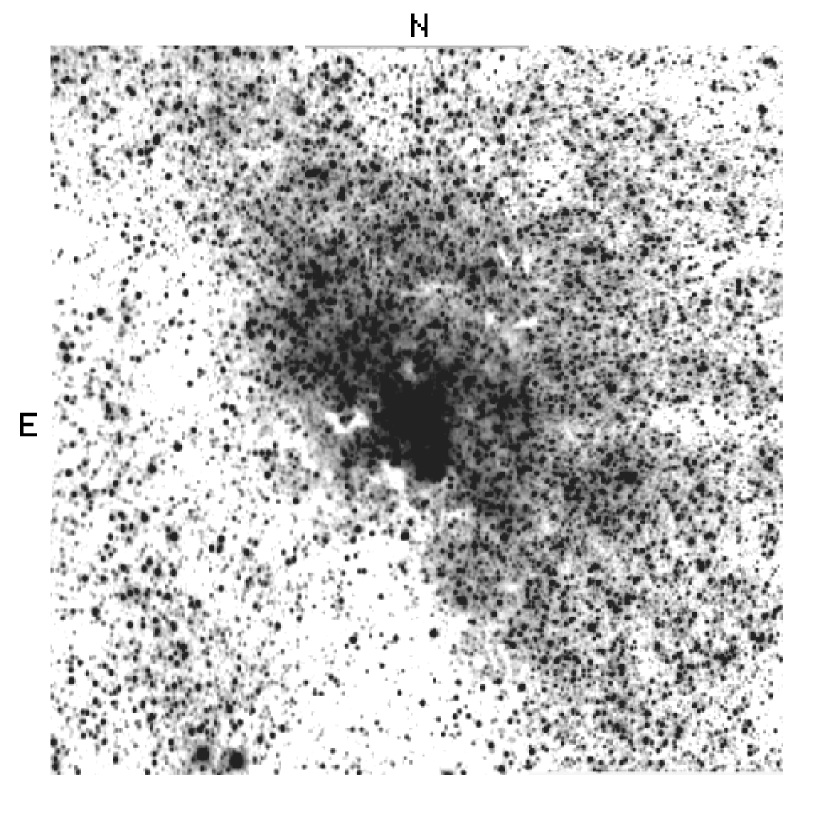
Figure 1: The final $K$ image of the $6.17\times 6.15$ arcmin mosaic field obtained at CTIO. The SgrA complex lies near the center of the field. The image quality is roughly 1.5 arcsec FWHM.

The images of the individual fields were then used to construct a mosaic covering $6\times 6$ arcmin. The FWHM of stars in overlapping portions of adjacent images were measured to assess differences in image quality, which were removed by convolving those frames having the smaller FWHM with a gaussian. Overlapping portions of adjacent frames were trimmed. The resulting $K$ mosaic, which has an image quality of $\sim 1.5$ arcsec FWHM, is shown in Figure 1. Variations in the line-of-sight extinction are plainly evident, illustrating the role that differential reddening plays in defining the photometric properties of objects near the GC.

2.2 MDM Data

The second dataset was recorded with the Ohio State University MOSAIC camera, which was mounted at the f/7.5 Cassegrain focus of the 2.4 metre MDM telescope, during the night of UT June 20 1997. MOSAIC contains a $1024\times 1024$ Alladin InSb array; however, only two of the detector quadrants were active, so that the total light-sensitive region was $512\times 1024$ pixels. Each pixel subtended 0.3 arcsec on a side, so that the imaged field is $2.6\times 5.1$ arcmin.

A single field, with SgrA* positioned near one end, was observed through $J,H,$ and $K$ filters. A complete observing sequence consisted of four exposures per filter, with the telescope pointing offset in a $10\times 10$ arcsec square dither pattern between individual integrations. Two sequences were recorded – one, intended to study bright stars, had a total integration time of 12 sec ($4\times 3$ sec) per filter. A second, deeper, sequence was obtained with total integration times of 240 sec ($4\times 60$ sec) in $J$, 60 sec ($4\times 15$ sec) in $H$, and 40 sec ($4\times 10$ sec) in $K$. A number of standard stars from the list published by Casali & Hawarden (1992) were also observed during the 4 night observing run.

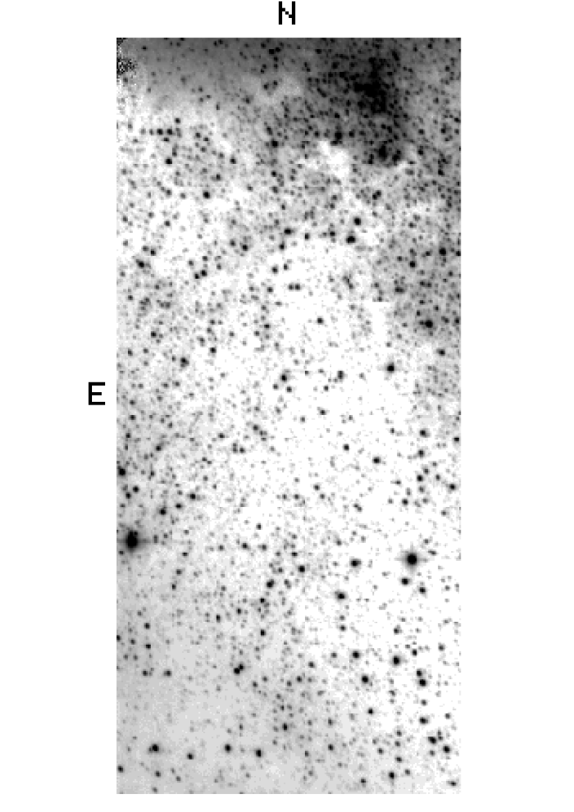
Figure 2: The final $K$ image of the $2.26\times 4.94$ arcmin field recorded with the MDM 2.4 metre telescope. The SgrA complex can be seen in the upper northwest corner of the field. The image quality is roughly 1.0 arcsec FWHM.

The data were reduced using the procedures described in §2.1. The final $K$ image, for which the image quality is $\sim 1.0$ arcsec FWHM, is shown in Figure 2. The upper two-thirds of this field overlap with the region observed at CTIO.

3 PHOTOMETRIC MEASUREMENTS

3.1 Stellar brightnesses and LFs

The brightnesses of individual standard stars were measured with the PHOT routine in DAOPHOT (Stetson 1987). The coefficients $\alpha$, $\beta$, and $\gamma$ in transformation equations of the form:

$M=m+\alpha X+\beta C+\gamma$

were determined using the method of least squares. $M$ and $m$ in this equation are the standard and instrumental brightnesses, $X$ is the airmass, and $C$ is the instrumental color. The night-to-night scatter in the standard star measurements was negligible. The residuals in the standard star measurements made at CTIO are $\pm 0.02$ mag for all filters. The residuals for the standard star measurements made at MDM are $\pm 0.02(J),\pm 0.06(H)$, and $\pm 0.05$ mag $(K)$.

The standard stars were selected so as to reduce possible sources of systematic error. In particular, standard stars were observed over the same airmass range as the GC – this is especially important for the measurements recorded at the MDM, as the GC never rises above 2 airmasses at that site. In addition, an effort was made to observe standard stars covering the broadest possible color range, although none of the standard stars have colors as red as the heavily obscured stars near the GC. The calibration of the CO index was checked by observing globular clusters in which individual stars have published CO measurements (Frogel, Persson, & Cohen 1983 and references therein).

Stellar brightnesses were measured with the PSF-fitting routine ALLSTAR (Stetson & Harris 1988), which is part of the DAOPHOT (Stetson 1987) photometry package. The calibrated brightnesses and colors are in good agreement with published values. This is demonstrated in Table 1, where the $K$ brightnesses of four bright ($K\leq 10$) IRS sources are compared with measurements made by Blum et al. (1996a). The mean difference is $\Delta K=-0.07\pm 0.14$, where the uncertainty is the error in the mean. Comparisons at other wavelengths show similar agreement.

Uncertainties in the photometric measurements were estimated by comparing the brightnesses of stars common to both the MDM and CTIO datasets. These comparisons indicate that the $K$ measurements have an uncertainty of $\pm 0.05$ mag when $K=10.5$, and $\pm 0.21$ mag at $K=13$. The mean difference in brightness between the MDM and CTIO measurements at moderately faint brightnesses is $\Delta K=-0.01\pm 0.02$ mag, where the difference is in the sense MDM – CTIO.

The $J,H,$ and $K$ LFs constructed from the CTIO and MDM datasets are plotted in Figure 3. Stars brighter than $K\sim 10$ are saturated in the deep MDM exposures, so the bright end of the MDM LFs were defined using the short exposure data. However, the detector in MOSAIC becomes significantly non-linear for count rates in excess of 10000 ADU/sec (Frogel 1998 – private communication), so caution should be exercised when interpreting the bright end ($K\leq 10$) of the MDM LFs. The linearity of the detector in CIRIM is well-calibrated, and the photometry from the CTIO data is reliable to $K\sim 8$.

Incompleteness causes the LFs to depart from power-laws at the faint end. For the CTIO data this occurs when $J=17.5$, $H=15.0$, and $K=13.5$. Incompleteness becomes significant about one mag fainter for the MDM data, owing to the longer integration times, better image quality, and larger telescope aperture. The completeness limits defined in this manner are averages over the entire field, and incompleteness sets in at brighter values in the high density SgrA environment.

Stars brighter than $K\sim 10$ in Figure 3 belong to the young SgrA complex or are disk objects. Indeed, the brightest M giants in BW, which are evolving on the AGB, have $K_{0}\sim 7$ (Frogel & Whitford 1987) which, if A${}_{K}\sim 3$ mag (DePoy & Sharpe 1991), corresponds to $K\sim 10$ near the GC. For comparison, stellar evolution models predict that the red giant branch tip for solar and higher metallicity old populations occurs near M${}_{K}\sim-7$ (Bertelli et al. 1994), which corresponds to $K\sim 10.5$ near the GC.

The dashed lines in Figure 3 show the trend defined by M giants in BW, as measured from Figure 17 of Tiede, Frogel, & Whitford (1995), shifted along the vertical axis to match the GC $K$ LFs near the faint end. Blum et al. (1996a) found that the power-law exponent at the faint end of the GC $K$ LF is similar to that in BW, and the excellent agreement between the GC and BW sequences in Figure 3 is consistent with this finding.

3.2 Color-Magnitude diagrams

The $(K,J-K)$, and $(K,H-K)$ CMDs constructed from the CTIO and deep MDM data are shown in Figures 4 and 5. Stars with $K\leq 10$ are saturated in the MDM data. The CMDs are dominated by a red plume comprised mainly of bulge giants, although a significant number of evolved young stars, which also have red colors, are concentrated in the SgrA complex (e.g. Davidge et al. 1997). Objects with $(J-K)\leq 2$ likely belong to the foreground disk.

The large line-of-site extinction in $J$ (A${}_{J}\sim 7.4$ mag) causes sample incompleteness to become significant at the color of the red plume on the $(K,J-K)$ CMD when $K\leq 12$. Nevertheless, although retricted to relatively bright stars, the $(K,J-K)$ CMD still provides an important means of comparing the photometric properties of the brightest giants in the inner bulge with those in BW. In the upper panel of Figure 6 the ridgeline defined from the CTIO ($K\leq 11.5$) and MDM ($K\geq 11.5$) $(K,J-K)$ CMDs, calculated using $\pm 0.25$ mag bins in $K$, is compared with the BW M giant sequence listed in Table 3B of Frogel & Whitford (1987). The two sequences can be brought into excellent agreement if $E(J-K)=4.4$ mag towards the inner bulge, which corresponds to A${}_{K}=2.9$ mag using the Rieke & Lebofsky (1985) reddening curve.

The ridgeline of the red plume on the $(K,H-K)$ CMDs, where incompleteness does not become significant until $K\sim 14$, is also well matched by the BW M giant sequence. This is demonstrated in the lower panel of Figure 6 where the locus of the ($K,H-K$) CMD, computed using $\pm 0.25$ mag bins in $K$, is compared with the BW M giant sequence from Table 3B of Frogel & Whitford (1987). The two sequences can be brought into excellent agreement if $E(H-K)=1.6$ mag for the inner bulge, which is consistent with the $(J-K)$ color excess derived from the $(K,J-K)$ CMD.

4 EXTINCTION-CORRECTED CO MEASUREMENTS

The comparisons in Figure 6 indicate that the brightest red giants in the inner bulge and BW have similar photometric properties, suggesting that the extinction towards the former can be estimated by adopting the intrinsic colors of the latter. Blum et al. (1996a) assumed that stars near the GC have colors that are the same as a ‘typical’ M giant in BW: $(J-H)_{0}=0.7$ and $(H-K)_{0}=0.3$. However, the current data samples stars spanning a wide range of intrinsic brightnesses, and hence colors, and this should be taken into account when computing A_K. Therefore, for the current study $(J-H)_{0}$ and $(H-K)_{0}$ were assigned using the M${}_{K}-$ color relations from Table 3B of Frogel & Whitford (1987). M_K was computed for each star by assuming that $\mu_{0}=14.5$ (Reid 1993) and A${}_{K}=2.9$ mag (§3.2). $(J-H)_{o}$ and $(H-K)_{o}$, and hence E$(J-H)$ and E$(H-K)$, were then calculated and used to compute an improved A_K based on the Rieke & Lebofsky (1985) reddening curve. Zero reddening was assigned to stars when A${}_{K}\leq 0$. These calculations were done only for the stars in the CTIO dataset.

It is likely that stars near the GC will have a range of metallicities, so that a single M${}_{K}-$ color relation will not apply to all objects. Given this possibility, it is of interest to investigate (1) how the A_K distribution changes if fiducial sequences other than those defined by BW giants are adopted, and (2) how these changes affect, for example, the distribution of reddening-corrected CO indices. Therefore, a second set of A_K values were computed using relations between M_K and near-infrared colors derived from the Frogel, Persson, & Cohen (1981) aperture measurements of 47 Tuc giants.

The histogram distribution of A_K values derived for stars in the CTIO field, shown in the upper panel of Figure 7, peaks near A${}_{K}\sim 2.8$, which corresponds to A${}_{V}=25.5$, and $E(B-V)=8.2$. The A_K distribution computed using the 47 Tuc M${}_{K}-$ color relations is shown as a dotted line in the top panel of Figure 7. Bright giants in 47 Tuc are bluer than stars in BW with the same M_K, so the A_K distribution computed from the 47 Tuc relations is shifted to slightly higher values; however, as demonstrated below, this difference has a negligible effect on the distribution of reddening-corrected CO indices.

A_K varies across the field, and there is a tendency for the extinction to be highest in the vicinity of the SgrA complex. The radial behaviour of A_K is shown in Figure 8, and it is evident that the radially-averaged A_K values, shown in the second panel from the top, increase when $r\leq 50$ arcsec. The SgrA complex contains a number of hot massive evolved stars, and it might be anticipated that these objects will skew $\overline{A_{K}}$ near SgrA* to smaller values. However, the evolved young stars near the GC have excess infrared emission, which causes their $H-K$ colors to be similar to those of red giants (Davidge et al. 1997). The mean value of A${}_{K}\sim 3.1$ mag derived here for the SgrA complex is in good agreement with other reddening estimates, which have relied on smaller sample sizes (e.g. DePoy & Sharpe 1991). That this area of locally heavy extinction is coincident with the SgrA complex suggests that the excess obscuring material may be local to the GC region, rather than occuring in the intervening disk. Nevertheless, the possibility that this excess extinction may be due to a fortuitously positioned dust cloud anywhere along the sight line can not be discounted. If the mean extinction towards the inner bulge is A${}_{K}\sim 2.8$ mag, then the excess extinction towards SgrA is $3.1-2.8=0.3$ mag in $K$.

Reddening-corrected CO indices, CO_o, were then computed for stars in the CTIO dataset assuming that $\frac{E_{CO}}{E_{BV}}=-0.04$ (Elias, Frogel, & Humphreys 1985). The resulting CO_o distribution, shown in the upper panel of Figure 9, peaks near CO${}_{o}\sim 0.28$ and is noticeably asymmetric, with an extended tail towards smaller CO_o values. The dotted line in the top panel shows the distribution predicted if the 47 Tuc brightness-color relations are used to estimate extinction, and the result is very similar to that produced with the BW brightness-color relations.

To investigate the effect that sample incompleteness has on the CO_o distribution, a second CO_o distribution was computed for brightnesses where the sample is complete. The extinction-corrected $K$ LF, shown in the top panel of Figure 10, indicates that the data are complete when $K_{o}\leq 9$, which corresponds to $K\leq 12$. The CO_o distribution for stars with $K_{o}<9$ is shown in the middle panel of Figure 9. The distribution derived from stars with $K_{o}<9$ is skewed towards higher CO_o values than that derived from the entire dataset, as expected given the surface-gravity sensitivity of the CO bands. Nevertheless, while a Kolmogoroff-Smirnoff test indicates that the two distributions are significantly different, both peak near CO${}_{o}=0.3$.

The LF in Figure 10 can be used to predict the distribution of CO_o values that would result if M giants in BW and near the GC have the same CO – M_K relation. The predicted CO_o distribution for stars with $K_{o}$ between 11.25 and 7.25 (the range of brightnesses covered by M giants in BW), calculated using the LF in Figure 10 and the CO–M_K relation from Table 3B of Frogel & Whitford (1987), is shown in the upper panel of Figure 11. The predicted distribution, which does not include the effects of observational errors, is visibly asymmetric, in the same sense as the observed distribution. It should also be noted that the predicted CO_o distribution automatically includes the effects of sample incompleteness, as the observed LF is used to set the number of stars with a given CO value.

In order to compare the observed and predicted CO_o distributions it is necessary to include the effects of observational errors in the latter. This was done by convolving the predicted CO_o distribution with a gaussian, the width of which was selected so that the number of stars with predicted CO indices between 0.16 and 0.28 matched those observed, and the result is shown in Figure 12. It is evident that the observed and predicted CO_o distributions have similar shapes. Although not plotted on Figure 12, the peak of the CO_o distribution predicted if stars near the GC followed the M${}_{K}-$ CO_o relation defined by bright giants in 47 Tuc occurs near CO${}_{o}\sim 0.15$, which is much smaller than what is observed. Consequently, the comparison in Figure 12 indicates that M giants in the central regions of the Galaxy and in BW follow the same M_K – CO relation. Moreover, the number of stars with CO indices similar to red giants in 47 Tuc must be very small.

Sellgren et al. (1990) and Haller et al. (1996) found that $2.3\mu$m CO absorption in unresolved sources weakens within 8 arcsec of SgrA*, a result that has been attributed to the presence of young main sequence stars (Eckart et al. 1995). The present data can be used to study radial trends among bright resolved sources in the SgrA complex, as well as search for radial CO_o variations among resolved sources over larger angular scales. In Figure 13 the CO_o indices for individual stars are plotted as a function of distance from SgrA*. There is significant scatter, and to help interpret these results the mean CO_o and $K_{o}$ values in 20 arcsec intervals are plotted in the middle and lower panel of this figure, with the errorbars showing the error of the mean. $<K_{o}>$ increases with radius when $r<100$ arcsec, due to the radial decrease in stellar density, and the corresponding shift of the completeness limit to fainter values. The solid squares in the middle panel show the CO index that is appropriate for $<K_{o}>$, based on the M${}_{K}-$ CO relation for M giants in BW.

It is evident from the middle panel of Figure 13 that $<CO_{o}>$ drops when $r<20$ arcsec, due to the concentration of bright young blue stars, which have little or no CO absorption, in the SgrA complex. However, there is excellent agreement between observed and predicted CO_o values for distances between 70 and 200 arcsec from SgrA*. While there is a tendency for $<CO_{o}>$ to increase when $r<220$ arcsec, the significance is low, as these measurements are based on only a small number of points. Therefore, the SgrA complex aside, there is no evidence for a radial departure from the BW M${}_{K}-$ CO relation in this field.

5 SUMMARY AND DISCUSSION

Moderately deep near-infrared images have been used to probe the bright ($K\leq 13.5$) stellar content in the central $6\times 6$ arcmin field of the Galaxy. The ridgeline of the bulge giant branch on the $(K,J-K)$ and $(K,H-K)$ CMDs is well matched by the BW M giant sequence, reddened according to the Rieke & Lebofsky (1985) extinction curve. This similarity in photometric properties suggests that the extinctions to individual stars in the inner bulge can be estimated by adopting the M${}_{K}-$ color relations defined by M giants in BW. The mean extinction outside of the SgrA complex, where A${}_{K}=3.1$ mag, is A${}_{K}=2.8$ mag. The extinction estimates for individual stars have been used to generate reddening-corrected CO indices, and the histogram distribution of CO_o values can be reproduced using the M${}_{K}-$ CO_o relation defined by M giants in BW. Therefore, M giants near the GC and in BW have similar $2.3\mu$m CO strengths.

A potential source of systematic error in the procedure used to compute A_K is that a single set of M${}_{K}-$ color relations have been used, and no attempt has been made to allow for a dispersion in the metallicities of giants in the central regions of the bulge. There is a selection effect for magnitude-limited samples, in the sense that the brightest stars in a field containing an old composite population are likely the most metal-rich, so the current data likely do not sample the full range of metallicities near the GC. In any event, the CO_o distribution does not change substantially when M${}_{K}-$ color relations defined by red giants in 47 Tuc ([Fe/H] $\sim-0.7$) are used to estimate extinction, indicating that the main conclusions of this paper are insensitive to the adopted intrinsic colors of GC giants.

Another source of systematic error is that the A_K values derived in §4 require measurements in $J,H$, and $K$. This broad wavelength coverage introduces a bias against heavily reddened objects, which are faint, and hence may not be detected, in $J$. In fact, there are regions where the extinction is so high that stars are not detected in $K$. The tendency to miss the most heavily reddened stars skews the A_K distribution to lower values. One way to reduce, but not entirely remove, this bias is to estimate extinction using only $H-K$ colors, for which the number of objects is over $3\times$ greater than those with $J$ measurements. Following the procedure described earlier, $(H-K)_{0}$ was assigned to each star using the $M_{K}-(H-K)$ relation for BW M giants, and the results are shown in the lower panels of Figures 7 – 12, while the radial distribution of CO_o values is plotted in Figure 14. It is evident from the lower panel of Figure 8 that a number of sources with relatively high A_K are added to the sample when measurements in $J$ are not required. Nevertheless, the impact on the CO_o distribution is negligible, indicating that stars with higher than average obscuration near the GC have $2.3\mu$m CO strengths that are similar to less heavily reddened stars.

It should be emphasized that the $2.3\mu$m CO bands provide only one diagnostic of chemical composition. Indeed, studies of the radial behaviour of the $2.3\mu$m CO bands in the bulges of other galaxies reveal weak or non-existant gradients (e.g. Frogel et al. 1978), even though many of these systems show line strength gradients at optical wavelengths. When interpreting this ostensibly contradictory result it should be recalled that the CO measurements are dominated by the brightest red stars which, in old populations, will be those that are the most metal-rich. If the most metal-rich population in the bulges of other galaxies follows a single M${}_{K}-$ CO relation with no radial dependence, as appears to be the case in the inner regions of the Galactic bulge, then this would help to explain why the wide-aperture CO measurements of other systems do not show gradients.

There are indications that the abundances of some species in the spectra of metal-rich giants may vary with distance from the GC. In particular, the infrared spectra obtained by Blum et al. (1996b) indicate that $2.3\mu$m CO absorption in GC giants is stronger than in BW stars having the same $2\mu$m Na and Ca absorption line strengths. Therefore, given that the CO line strengths in giants near the GC are similar to those in BW, then the Blum et al. measurements are suggestive of radial changes in [Na/Fe] and [Ca/Fe] among bulge stars.

While this paper has concentrated on bulge stars, a modest disk population is also evident in the CMDs, and these data can be used to estimate the contribution disk objects make to the near-infrared light output near the GC. Objects with $(J-K)\leq 2.5$ and brightnesses between $K\sim 7.5$ (the approximate saturation limit of the CTIO data) and $K\sim 12$ (the faintest point at which the CTIO $K,J-K$ CMD is complete over a broad range of colors) account for 2.6% of the total light from resolved sources within 3 arcmin of the GC. The relative contribution made by disk stars would be much lower if dust did not obscure the bulge. Assuming that (1) the disk stars are not heavily reddened, and (2) stars near the GC are obscured by A${}_{K}\sim 2.8$ mag then, after correcting for this extinction, the contribution from disk stars drops to only 0.05% when $K_{0}\leq 8.5$.

Sincere thanks are extended to the referee, Jay Frogel, for providing comments that greatly improved the paper.

IRS #	KTD	KBSD	$\Delta$
7	6.44	6.55	$-0.11$
9	8.80	8.57	0.23
16NE	8.56	9.01	$-0.45$
28	9.41	9,36	0.05

Table 1: Comparison with $K$ measurements obtained by Blum et al. (1996a)

Figure 3: $J,H,$ and $K$ LFs constructed from the CTIO (left column) and MDM (right column) datasets. The error bars show the uncertainties due to counting statistics. $n$ is the number of stars per square arcmin per mag. The dashed line in the bottom row shows the trend defined by bright giants in BW, shifted by an arbitrary amount along the vertical axis to match the observations between $K=10$ and 13.

Figure 4: $(K,J-K)$ CMDs for the CTIO and deep (60 sec integration times in $J$ and 10 sec in $K$) MDM datasets. Stars brighter than $K=10$ are saturated in the MDM data.

Figure 5: $(K,H-K)$ CMDs for the CTIO and deep (15 sec integration times in $H$ and 10 sec in $K$) MDM datasets. Stars brighter than $K=10$ are saturated in the MDM data.

Figure 6: Comparison between the BW M giant sequence and the GC giant branch locus on the $(K,J-K)$ (top panel) and $(K,H-K)$ (bottom panel) CMDs. The ridgeline of the GC giant branch is shown as crosses, while the filled squares are the BW M giant sequence listed in Table 3B of Frogel & Whitford (1987). The open squares show the BW sequence as it would appear if A${}_{K}=2.9$ mag. Note that the GC and BW sequences have very similar shapes.

Figure 7: The histogram distribution of A_K values, derived assuming that red giants in BW and the inner bulge follow the same M${}_{K}-$ color relations. The top panel shows the distribution that results if extinctions are computed using both $J-H$ and $H-K$ colors, while the lower panel shows the A_K distribution if only $H-K$ colors are used. The dotted line in the upper panel is the A_K distribution if extinctions are estimated using M${}_{K}-$ color relations defined by 47 Tuc giants. The dashed line in the lower panel shows the A_K distribution from the upper panel, scaled to match the number of stars having only $H-K$ colors. Note that the A_K distribution derived only from $H-K$ includes more highly reddened objects, due to the deeper nature of the $H$ and $K$ images.

Figure 8: A_K as a function of distance from SgrA*. The top panel shows A_K for individual stars computed using both $J-H$ and $H-K$ colors, while the means in 20 arcsec annuli, with errorbars indicating the standard deviation of the mean, are plotted in the second panel from the top. Note the tendency for A_K to increase towards smaller radii. The lower two panels show the A_K values that result if only $H-K$ colors are used.

Figure 9: CO_o distributions calculated using the A_K values shown in Figure 7. The top two panels show the distributions that result if extinctions are computed using both $J-H$ and $H-K$ colors, while the lower panel shows the CO_o distribution if only $H-K$ colors are used. The distribution in the middle panel is restricted to stars with $K_{o}<9$, where the data are complete. The dotted line in the upper panel is the CO_o distribution that results if extinction is estimated from the 47 Tuc M${}_{K}-$ color relation. The dashed lines in the lower two panels show the CO_o distribution from the upper panel, scaled to correct for differences in sample size.

Figure 10: The reddening-corrected K_o LFs, generated using the A_K values shown in Figure 7. The dashed line in the lower panel shows the LF from the upper panel, scaled to match the number of stars having only $H-K$ colors. Note that the two LFs are very similar after accounting for differences in sample size.

Figure 11: The CO_o distributions predicted from the M${}_{K}-CO$ relation given in Table 3B of Frogel & Whitford (1987). These curves, which do not include the effects of observational errors in the CO indices, were constructed using the K_o LFs shown in Figure 10 for stars with K_o between 11.25 and 7.25.

Figure 12: The CO_o distribution for stars with $K_{o}$ between 11.25 and 7.25, which corresponds to the brightness range of M giants in BW. The top panel shows the CO_o distribution if extinctions are computed using both $J-H$ and $H-K$ colors, while the lower panel shows the CO_o distribution that results if only $H-K$ colors are used. The dashed line in each panel shows the predicted CO_o distributions from Figure 11, smoothed to match the observed number of stars with CO_o between 0.16 and 0.28.

Figure 13: The top panel shows CO_o as a function of distance from SgrA* for stars with extinctions estimated from both $J-H$ and $H-K$ colors. The mean values of CO_o and $K_{o}$ in 20 arcsec intervals are plotted as crosses in the middle and lower panels, with the errorbars showing the uncertainty in the mean. The filled squares in the middle panel are the CO_o values predicted from $<K_{o}>$, based on the M${}_{K}-CO$ relation defined by M giants in BW.

Figure 14: Same as Figure 13, except for stars that had extinctions estimated from $H-K$ colors only.

References

- (1)
- (2) Allen, D. A. 1994, The Nuclei of Normal Galaxies: Lessons from the Galactic Center, R. Genzel & A. I. Harris, Dordrecht:Reidel, 293
- (3)
- (4) Bergbusch, P. A., & VandenBerg, D. A. 1992, ApJS, 81, 163
- (5)
- (6) Bertelli, G., Bressan, A., Chiosi, C., Fagotto, F., & Nasi, E. 1994, A&A Rev., 106, 275
- (7)
- (8) Blanco, V. M., & Terndrup, D. M. 1990, AJ, 98, 843
- (9)
- (10) Blum, R. D., Sellgren, K., & DePoy, D. L. 1996a, ApJ, 470, 864
- (11)
- (12) Blum, R. D., Sellgren, K., & DePoy, D. L. 1996b, AJ, 112, 1988
- (13)
- (14) Carr, J. S., Sellgren, K., & Balachandran, S. C. 1996, The Galactic Center, ASP Conf. # 102, R. Gredel, 212
- (15)
- (16) Casali, M., & Hawarden, T. 1992, JCMT-UKIRT Newsletter, 4, 33
- (17)
- (18) Davidge, T. J. 1997, AJ, 113, 985
- (19)
- (20) Davidge, T. J., Simons, D. A., Rigaut, F., Doyon, R., & Crampton, D. 1997, AJ, 114, 2586.
- (21)
- (22) DePoy, D. L., & Sharpe, N. A. 1991, AJ, 101, 1324
- (23)
- (24) Eckart, A., Genzel, R., Hofmann, R., Sams, B. J., & Tacconi-Garman, L. E. 1995, ApJ, 407, L23
- (25)
- (26) Elias, J. H., Frogel, J. A., & Humphreys, R. M. 1985, ApJS, 57, 91
- (27)
- (28) Elias, J. H., Frogel, J. A., Matthews, K., & Neugebauer, G. 1982, AJ, 87, 1029
- (29)
- (30) Frogel, J. A., & Whitford, A. E. 1987, ApJ, 320, 199
- (31)
- (32) Frogel, J. A., Persson, S. E., & Cohen, J. G. 1981, ApJ, 246, 842
- (33)
- (34) Frogel, J. A., Persson, S. E., & Cohen, J. G. 1983, ApJS, 53, 713
- (35)
- (36) Frogel, J. A., Persson, S. E., Aaronson, M., & Matthews, K. 1978, ApJ, 220, 75
- (37)
- (38) Haller, J. W., Rieke, M. J., Rieke, G. H., Tamblyn, P., Close, L., & Melia, F. 1996, ApJ, 456, 194
- (39)
- (40) Hodapp, K.-W., Rayner, J., & Irwin, E. 1992, PASP, 104, 441
- (41)
- (42) Kraft, R. P. 1994, PASP, 106, 553
- (43)
- (44) Minniti, D., Olszewski, E. W., Liebert, J., White, S. D. M., Hill, J. M., & Irwin, M. J. 1995, MNRAS, 277, 1293
- (45)
- (46) Morris, M., & Serabyn, E. 1996, ARA&A, 34, 645
- (47)
- (48) Reid, M. 1993, ARA&A, 31, 345
- (49)
- (50) Rieke, G. H., & Lebofsky, M. J. 1985, ApJ, 288, 618
- (51)
- (52) Saha, P., Bicknell, G. V., & McGregor, P. J. 1996, ApJ, 467, 636
- (53)
- (54) Sellgren, K., McGinn, M. T., Becklin, E. E., & Hall, D. N. B. 1990, ApJ, 359, 112
- (55)
- (56) Stetson, P. B. 1987, PASP, 99, 191
- (57)
- (58) Stetson, P. B., & Harris, W. E. 1988, AJ, 96, 909
- (59)
- (60) Tiede, G. P., Frogel, J. A., & Whitford, A. E. 1995, AJ, 110, 2788
- (61)
- (62) van den Bergh, S. 1989, ARA&A, 1, 111
- (63)