Multi-frequency Wiener filtering of CMB data with polarization and estimation of cosmological parameters

We present a method of subtracting the foreground contamination for the measurement of CMB polarization. We calculate the resultant errors on CMB polarization and temperature-polarization cross correlation power spectra for the high frequency instrument (HFI) aboard Planck Surveyor, and estimate the corresponding errors on cosmological parameters

1 Introduction

The upcoming satellite CMB experiment Planck surveyor offers an unprecedented opportunity to measure CMB polarization. A major hurdle in extracting the primary CMB signal from data, apart from noise, is galactic and extragalactic foregrounds. However, as the foregrounds differ from CMB in both frequency dependence and spatial distribution, one can hope to reduce their level in a multi-frequency CMB experiment. A multi-frequency Wiener filtering method to implement this scheme was developed $\!{}^{{\bf?},{\bf?}}$ and applied to cleaning the simulated CMB temperature map by Bouchet et al. $\!{}^{{\bf?}}$. They showed that the residual contamination after cleaning the map is much smaller than the CMB primary signal, and therefore the foregrounds may not be a major obstacle in the extraction of CMB temperature angular power spectrum. However, as the CMB polarization signal is expected to be one to two orders of magnitudes below the temperature signal, it is likely to be comparable to both the experimental noise and the level of foregrounds. Sethi et al. $\!{}^{{\bf?}}$ modelled and estimated the level of dust polarized emission at high galactic latitudes. Dust polarization is expected to be the dominant contaminant for measuring CMB polarization using Planck HFI.

In this paper, we extend the multi-frequency Wiener filtering method to include the polarization and temperature-polarization cross-correlation. The aim of this exercise is to quantify errors in estimating various power spectra and consequently the errors in cosmological parameters. Our results are relevant for Planck HFI.

2 Multi-frequency Wiener filtering on CMB data

Let us denote the observed data at different frequencies as, $y_{\nu}^{i}$, where $\nu$ indicates the frequency of the instrumental channel, and $i$ the nature of the observed field (temperature $T$ and $E$-mode polarization$\!{}^{{\bf?}}$). $y_{\nu}^{i}$, for a given $i$, takes contributions from various galactic and extragalactic sources, apart from the primary CMB signal and instrumental noise. Let us call $x_{p}^{j}$ the contribution of the field $j$ due to process $p$, this is the quantity we want to recover from the observational data $y_{\nu}^{i}$. We assume that there is a linear relation between them. In multipole space, it can be expressed as:

$$y_{\nu}^{i}(l,m)=A_{\nu p}^{ij}(l,m)x_{p}^{j}(l,m)+b_{\nu}^{i}(l,m)$$ (1)

where $A_{\nu p}^{ij}$ is the instrument response kernel, and $b_{\nu}^{i}$ is the detector noise level per pixel for the full mission time (all repeated indices are summed over).

The problem is now how to construct an optimal estimator $\hat{x}_{p}^{j}$. We chose this estimator to be linear in the observed data:

$$\hat{x}_{p}^{i}=W_{p\nu}^{ij}y_{\nu}^{j}$$ (2)

The reconstruction error for a given field and process is given by $|(\hat{x}_{p}^{i}-x_{p}^{i})^{2}|\equiv(\varepsilon_{p}^{i})^{2}$. $W_{p\nu}^{ij}$ is chosen so as to make the variance of the reconstruction error minimal. The derivatives of the error with respect to the filters coefficients $W_{p\mu}^{ic}$ should then be zero. This condition can be expressed as:

$$A_{\mu p^{\prime}}^{ck}W_{p\nu^{\prime}}^{il}A_{\nu^{\prime}p^{\prime\prime}}^{lm}\langle x_{p^{\prime}}^{k}x_{p^{\prime\prime}}^{m}\rangle+W_{p\nu^{\prime}}^{ib}\langle b_{\mu}^{c}b_{\nu^{\prime}}^{b}\rangle=A_{\mu p^{\prime}}^{ck}\langle x_{p^{\prime}}^{k}x_{p}^{i}\rangle.$$ (3)

2.1 Implementation of foregrounds removal

Eq. (3) is valid for the general case in which various processes, fields, and corresponding instrumental noises could be correlated. We consider here only uncorrelated processes and noises between different fields and channels. We allow for the correlation between the two fields $T$ and $E$. With these conditions, Eq. (3) can be written as a system of four matrix equations which can be solved by substitution.

Bouchet et al. $\!{}^{{\bf?}}$ defined a quantity called the ’quality factor’ to understand the quality of extraction of the signal corresponding to a given process. A straightforward generalisation of the quality factor, valid for multiple fields, can be written as:

$$Q_{pp^{\prime}}^{ij}=\frac{\langle\hat{x}_{p}^{i}\hat{x}_{p^{\prime}}^{j}\rangle}{\langle x_{p}^{i}x_{p^{\prime}}^{j}\rangle}=W_{p\nu}^{ik}A_{\nu p^{\prime\prime}}^{kl}\langle x_{p^{\prime\prime}}^{l}x_{p^{\prime}}^{j}\rangle$$ (4)

where we have used Eq. (3) to write the second equality. ${\mathbf{Q}}^{11}$ and ${\mathbf{Q}}^{22}$ can readily be interpreted as the quality of the reconstruction of temperature and polarization maps, respectively. It should be noted that in the presence of cross-correlations, the quality factor of either field is better than the case without cross-correlations. Though the reconstruction of temperature maps is only slightly changed by cross-correlation term, the quality of polarization reconstruction gets a big boost from the presence of temperature-polarization cross-correlation. However the meaning of term ${\mathbf{Q}}^{21}$ (and ${\mathbf{Q}}^{12}$) is not apparent. Much of the contribution to ${\mathbf{Q}}^{12}$ comes from the term with ${\mathbf{W}}^{11}$, and therefore it is very close to the quality factor for the extraction of temperature and is nearly independent of the polarization noise. It is not surprising as it merely tells us that to optimally reconstruct the cross-correlation one needs to throw out the noisy data, i.e. the polarization. However, the quantity of interest for us is the error in the extraction of the power spectrum of cross-correlation, which should not be confused with ${\mathbf{Q}}^{12}$. To get a real idea of the error bars of the different spectra, we must define estimators of those power spectra from the filtered data, and compute their covariance.

2.2 Unbiased estimators of power spectra

$\hat{x}_{p}^{i}$ (Eq. (2)) is the data obtained after performing Wiener filtering on the multi-frequency maps. Our aim in this section is to use this data to write an unbiased estimator of the true power spectrum $x_{p}^{i}$. The average power spectrum of $\hat{x}_{p}^{i}$ can be written as:

$$\langle\hat{x}_{p}^{i}\hat{x}_{p}^{i}\rangle=W_{p\nu}^{ij}W_{p\nu^{\prime}}^{il}\left[A_{\nu p^{\prime}}^{jk}A_{\nu^{\prime}p^{\prime\prime}}^{lm}\langle x_{p}^{i}x_{p}^{i}\rangle+\langle b_{\nu}^{j}b_{\nu^{\prime}}^{l}\rangle\right]$$ (5)

This can be expanded to give:

$$\langle\hat{x}_{p}^{i}\hat{x}_{p}^{j}\rangle=(Z_{p}^{ij}C_{p}^{ij}+b_{p}^{ij})=Q_{p}^{ij}C_{p}^{ij}$$ (6)

Here $\{i,j\}$ stand for $T$ and $E$. $b_{p}^{ij}$ are generalized versions of the instrumental noise, containing contributions of the noise from different channels as well as some power leakage of the other processes and the other fields. We then define unbiased estimators of the spectra:

$$\hat{C}_{p}^{ij}=\frac{1}{Z_{p}^{ij}}\left(\frac{1}{2\ell+1}\sum_{m}\|\hat{x}_{p}^{i}(m)\hat{x}_{p}^{j}(m)\|-b_{p}^{ij}\right)$$ (7)

and compute their covariances:

$$Cov(\hat{C}_{p}^{TT}) = \frac{2}{2\ell+1}\left(C_{p}^{TT}Q_{p}^{11}/Z_{p}^{11}\right)^{2}$$ (8)

$$Cov(\hat{C}_{p}^{EE}) = \frac{2}{2\ell+1}\left(C_{p}^{EE}Q_{p}^{22}/Z_{p}^{22}\right)^{2}$$ (9)

$$Cov(\hat{C}_{p}^{TE}) = \frac{1}{2\ell+1}\frac{\left((Q_{p}^{12})^{2}(C_{p}^{TE})^{2}+Q_{p}^{11}Q_{p}^{22}C_{p}^{TT}C_{p}^{TE}\right)}{(Z_{p}^{12})^{2}}$$ (10)

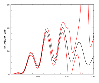
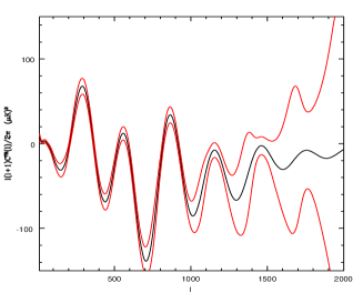
It has been assumed that both CMB and foregrounds are Gaussian fields in the computation of covariances. In Fig. 1 we show the E-mode polarization and $ET$ cross-correlation power spectra for sCDM model and the expected $1\sigma$ errors on their measurement using the specifications of Planck HFI. Apart from polarized dust, an additional contribution to polarized foregrounds from $40\%$ polarized synchrotron emission has been assumed. As the synchrotron foreground is subdominant at HFI frequencies, it doesn’t affect our results. However, it is expected to be the major foreground for MAP and Planck low frequency instrument (LFI).

Figure 1: Power spectra and $1\sigma$ errors for the E-mode polarization and the temperature-polarization cross-correlation respectively.

3 Errors on cosmological parameters

The unbiased estimators defined above and their covariances can be used to estimate the precision we expect on the measurement of cosmological parameters once the foregrounds are filtered out for any desired experiment.

3.1 Fisher Matrix

The Fisher matrix is defined as an average value of the second derivatives of the logarithm of the Likelihood function with respect to the cosmological parameters, taken at the maximum likelihood point:

$$F_{ij}=\left\langle\frac{\partial^{2}\mathcal{L}}{\partial\theta_{i}\partial\theta_{j}}\right\rangle_{\Theta=\Theta_{0}}$$ (11)

One can take this matrix as an estimate of the covariance matrix of the cosmological parameters. Following Zaldarriaga et al. $\!{}^{{\bf?}}$ we generalize the Fisher matrix approach to the polarized case. It can be written as:

$$F_{ij}=\sum_{\ell=2}^{+\infty}\sum_{X,Y}\frac{\partial C_{\ell}^{X}}{\partial\theta_{i}}\rm{Cov}^{-1}\left(C_{\ell}^{X},C_{\ell}^{Y}\right)\frac{\partial C_{\ell}^{Y}}{\partial\theta_{j}}$$ (12)

where $\rm{Cov}(C_{\ell}^{X},C_{\ell}^{Y})$ stands for the covariance matrix of the power spectra estimators, and $\{X,Y\}\in\{T,E,TE\}$. We will then use the covariances computed for the unbiased estimators defined in the previous section to take into account the foregrounds removal in the error bars computation.

With the present specifications of Planck HFI, our results are shown in Table 1 for a variant of CDM model. The best channel case corresponds to $\nu=143\,\rm GHz$ channel with no foregrounds and the worst case corresponds to the same channel with foregrounds added as noise. As is clearly seen, significant improvement on parameter estimation can be achieved if the foregrounds are removed using the Wiener filtering technique discussed in previous sections, except for the optical depth to the last scattering surface $\tau$. An accurate determination of such small values of $\tau$ depends on the level of CMB polarization at $\ell\leq 10$, which in our case is dominated by polarized foregrounds which cannot be easily removed. And therefore, a careful analysis of polarized foregrounds at large scales is necessary to determine such a small value of $\tau$. The different power spectra were computed with the CMB Boltzmann code CMBFAST $\!{}^{{\bf?}}$.

Table 1: Errors on cosmological parameters. $\Delta\Omega_{\Lambda}$ is given in absolute value.

Parameters	$C_{2}$	$h$	$\Omega_{b}$	$\Omega_{\Lambda}$	$\tau$	$n_{s}$	$n_{t}$	$T/S$
Model	$796(\mu K)^{2}$	$0.5$	$0.05$	$0.0$	$0.05$	$0.99$	$0.01$	$0.1$
Worst case	$3.72$ %	$1.11$ %	$1.93$ %	$0.032$	$28.3$ %	$0.40$ %	$538$ %	$78.0$ %
Best channel	$2.5$ %	$1.07$ %	$1.87$ %	$0.031$	$2.74$ %	$0.38$ %	$453$ %	$67.6$ %
Wiener	$1.98$ %	$0.23$ %	$0.34$ %	$6.6\,10^{-3}$	$19.7$ %	$0.10$ %	$242$ %	$27.0$ %

References

- [1] F. R. Bouchet et al. , Space Science Rev. 74, 37(1995).
- [2] M. Tegmark and G. Efstathiou, ApJ 281, 1297 (1996).
- [3] S. K. Sethi, S. Prunet, and F. R. Bouchet, this volume.
- [4] M. Zaldarriaga, D. N. Spergel, and U. Seljak, ApJ 488, 1 (1997).
- [5] U. Seljak, ApJ 482, 6 (1997).
- [6] U. Seljak and M. Zaldarriaga,ApJ 469, 437 (1996)