GRAVITATIONAL LENSING EFFECT ON COSMIC MICROWAVE BACKGROUND POLARIZATION

Abstract

We investigate the effect of gravitational lensing by matter distribution in the universe on the cosmic microwave background (CMB) polarization power spectra and temperature-polarization cross-correlation spectrum. As in the case of temperature spectrum gravitational lensing leads to smoothing of narrow features and enhancement of power on the damping tail of the power spectrum. Because acoustic peaks in polarization spectra are narrower than in the temperature spectrum the smoothing effect is significantly larger and can reach up to 10% for $l<1000$ and even more above that. A qualitatively new feature is the generation of $B$ type polarization even when only $E$ is intrinsically present, such as in the case of pure scalar perturbations. This may be directly observed with Planck and other future small scale polarization experiments. The gravitational lensing effect is incorporated in the new version (2.4) of CMBFAST code.

I Introduction

Over the next few years a number of ground based, balloon and satellite experiments will measure CMB sky with an unprecedented accuracy and detail. The promise of a one percent precision on the measured power spectrum of CMB anisotropies requires a similar accuracy in the theoretical predictions, if we are to exploit all the information present in the data. The rewards will be rich: among other things this will allow an accurate determination of a number of cosmological parameters and testing of current structure formation theories [1]. In principle such a program is possible, since the anisotropies were produced when the universe was still in the linear regime, which makes the calculations of model predictions very accurate. In practice there are a number of important effects that need to be included if this goal is to be realized. One of the most important among these is the gravitational lensing effect.

As photons propagate through the universe from their last scattering to our detectors they are randomly deflected by the gravitational force exerted upon them by the inhomogeneous mass distribution. Previous work has shown that gravitational lensing has an effect on the temperature anisotropy power spectrum which is not insignificant [2, 3]. The random deflections smear out the sharp features in the correlation function or power spectrum, leading to a suppression of acoustic oscillations. Gravitational lensing can also enhance power on the damping tail, causing it to decay less rapidly than predicted on very small angular scales [4]. Gravitational lensing effect on the temperature anisotropies has been discussed several times in the literature and the formalism to calculate it using the evolution of density power spectrum both in linear and nonlinear regime has been presented in [3]. In this paper we extend this calculation to the two linear polarization power spectra and to the cross-correlation spectrum between temperature and polarization. Because acoustic oscillations are narrower for polarization spectra than for temperature, one expects gravitational lensing effect to be more significant in the former and indeed our results confirm this. In addition, a qualitatively new effect is the mixing between $E$ and $B$ types of polarization, which changes the pattern of polarization. The outline of the paper is the following. In §II we develop the formalism: this section contains all the main analytic expressions needed for a numerical implementation of the effect. These have been numerically implemented in the new version of CMBFAST package (version 2.4) and require only a marginal increase in the CPU time for their evaluations. In §III we compute the effect for a typical cosmological model and address the question of direct observability of the effect. We present the conclusions in §IV.

II Two-point correlators in the presence of lensing

The large scale density fluctuations in the universe induce random deflections in the direction of the CMB photons as they propagate from the last scattering surface to us. This alters the power spectrum of both the temperature and polarization anisotropies. The quantity is responsible for the deflections is the projected surface density. Since the structures are not very correlated on large scales the gravitational lensing effect is only relevant at the small angular scales in the CMB. We may hence use the small scale limit formalism [3], which simplifies the calculations.

The observed CMB temperature in the direction $\theta$ is $T({\hbox{\boldmath{$\theta$}}})$ and equals the unobservable temperature at the last scattering surface $\tilde{T}({\hbox{\boldmath{$\theta$}}}+\delta{\hbox{\boldmath{$\theta$}}})$, where $\delta{\hbox{\boldmath{$\theta$}}}$ is the angular excursion of the photon as it propagates from the last scattering surface until the present. In terms of Fourier components we have

$$T({\hbox{\boldmath{$\theta$}}}) = \tilde{T}(\hbox{\boldmath{$\theta$}}+\delta{\hbox{\boldmath{$\theta$}}})$$ (1)

$$= (2\pi)^{-2}\int d^{2}{\hbox{\boldmath{$l$}}}\ e^{i{\hbox{\boldmath{$l$}}}\cdot(\hbox{\boldmath{$\theta$}}+\delta{\hbox{\boldmath{$\theta$}}})}\ T({\hbox{\boldmath{$l$}}}).$$ (2)

The same relation applies to the two Stokes parameters $Q$ and $U$ that describe linear polarization [6]. In the small scale limit we take the direction of observation to be near $\hat{\hbox{\boldmath{$z$}}}$ and we orient the local coordinate system orthogonal to $\hat{\hbox{\boldmath{$z$}}}$ to define $Q$ and $U$: $Q$ is the difference between the photon intensities along $\hat{\hbox{\boldmath{$x$}}}$ and $\hat{\hbox{\boldmath{$y$}}}$, while $U$ is the difference between photon intensities along the two diagonals. In terms of Fourier components these can be expressed with opposite parity Fourier components $E({\hbox{\boldmath{$l$}}})$ and $B({\hbox{\boldmath{$l$}}})$ [7]

$$Q({\hbox{\boldmath{$\theta$}}}) = \tilde{Q}({\hbox{\boldmath{$\theta$}}}+\delta{\hbox{\boldmath{$\theta$}}})$$ (3)

$$= (2\pi)^{-2}\int d^{2}{\hbox{\boldmath{$l$}}}\ e^{i{\hbox{\boldmath{$l$}}}\cdot({\hbox{\boldmath{$\theta$}}}+\delta{\hbox{\boldmath{$\theta$}}})}\ [E({\hbox{\boldmath{$l$}}})\cos(2\phi_{\hbox{\boldmath{$l$}}})-B({\hbox{\boldmath{$l$}}})\sin(2\phi_{\hbox{\boldmath{$l$}}})]$$ (4)

$$U({\hbox{\boldmath{$\theta$}}}) = \tilde{U}({\hbox{\boldmath{$\theta$}}}+\delta{\hbox{\boldmath{$\theta$}}})$$ (5)

$$= (2\pi)^{-2}\int d^{2}{\hbox{\boldmath{$l$}}}\ e^{i{\hbox{\boldmath{$l$}}}\cdot({\hbox{\boldmath{$\theta$}}}+\delta{\hbox{\boldmath{$\theta$}}})}\ [E({\hbox{\boldmath{$l$}}})\sin(2\phi_{\hbox{\boldmath{$l$}}})+B({\hbox{\boldmath{$l$}}})\cos(2\phi_{\hbox{\boldmath{$l$}}})].$$ (6)

The Fourier components satisfy

$$\langle\tilde{X}({\hbox{\boldmath{$l$}}})\tilde{X}({\hbox{\boldmath{$l$}}}^{\prime})\rangle=(2\pi)^{2}\ C_{\tilde{X}l}\ \delta^{D}({\hbox{\boldmath{$l$}}}-{\hbox{\boldmath{$l$}}}^{\prime}),$$ (7)

with $\tilde{X}=\tilde{T},\tilde{E},\tilde{B}$ and the average is over different realizations of the CMB field.

The correlation function of the temperature between two points in the sky, ${\hbox{\boldmath{$\theta$}}^{A}}$ and ${\hbox{\boldmath{$\theta$}}^{B}}$, only depends on their angular separation ${\theta}$. With our choice of coordinate system the correlations between the polarization variables are also a function of azimuthal angle $\phi$ [7]. This is not the natural coordinate system in which to define these correlation functions. Instead one should align the local coordinate system with the great circle that connects the two points [8]. With this choice parity conservation requires $T$ and $Q$ to be uncorrelated with $U$ and the correlation functions only depend on separation ${\theta}$. To obtain this set of correlation functions in our coordinate system we can calculate the correlation between the variables at the origin and another point separated by an angle ${\theta}$ along the $x$ axis. The correlation functions are calculated from equations (6) and (7),

$$C_{T}({\theta}) = \int{d^{2}{\hbox{\boldmath{$l$}}}\over(2\pi)^{2}}\ e^{il\theta\cos\phi_{l}}\langle e^{i{\hbox{\boldmath{$l$}}}\cdot(\delta{\hbox{\boldmath{$\theta$}}^{A}}-\delta{\hbox{\boldmath{$\theta$}}}^{B})}\ \rangle\ \ C_{\tilde{T}l}$$ (8)

$$C_{Q}({\theta}) = \int{d^{2}{\hbox{\boldmath{$l$}}}\over(2\pi)^{2}}\ e^{il\theta\cos\phi_{l}}\langle e^{i{\hbox{\boldmath{$l$}}}\cdot(\delta{\hbox{\boldmath{$\theta$}}^{A}}-\delta{\hbox{\boldmath{$\theta$}}}^{B})}\ \rangle\ \ [C_{\tilde{E}l}\cos^{2}(2\phi_{\hbox{\boldmath{$l$}}})+C_{\tilde{B}l}\sin^{2}(2\phi_{\hbox{\boldmath{$l$}}})]$$ (9)

$$C_{U}({\theta}) = \int{d^{2}{\hbox{\boldmath{$l$}}}\over(2\pi)^{2}}\ e^{il\theta\cos\phi_{l}}\langle e^{i{\hbox{\boldmath{$l$}}}\cdot(\delta{\hbox{\boldmath{$\theta$}}^{A}}-\delta{\hbox{\boldmath{$\theta$}}}^{B})}\ \rangle\ \ [C_{\tilde{E}l}\sin^{2}(2\phi_{\hbox{\boldmath{$l$}}})+C_{\tilde{B}l}\cos^{2}(2\phi_{\hbox{\boldmath{$l$}}})]$$ (10)

$$C_{C}({\theta}) = \int{d^{2}{\hbox{\boldmath{$l$}}}\over(2\pi)^{2}}\ e^{il\theta\cos\phi_{l}}\langle e^{i{\hbox{\boldmath{$l$}}}\cdot(\delta{\hbox{\boldmath{$\theta$}}^{A}}-\delta{\hbox{\boldmath{$\theta$}}}^{B})}\ \rangle\ \ C_{\tilde{C}l}\cos(2\phi_{\hbox{\boldmath{$l$}}}).$$ (11)

The remaining average in equation (11) is over the lensing fluctuations. Only the cross-correlation between $Q$ and $T$ is different from zero and we denote it $C_{C}({\theta})$. Even in the presence of lensing $U$ does not cross correlate with either $T$ or $Q$ because these quantities have opposite parities.

The correlation function of the excursion angle can be used to calculate the expectation value in equation (11) [3],

$$\langle\exp\{i{\hbox{\boldmath{$l$}}}(\delta{\hbox{\boldmath{$\theta$}}}-\delta{\hbox{\boldmath{$\theta$}}}^{\prime})\}\ \rangle = \exp\{-{l^{2}\over 2}[\sigma_{0}^{2}(\theta)+\cos(2\phi_{\hbox{\boldmath{$l$}}})\sigma_{2}^{2}(\theta)]\}$$ (12)

$$\approx 1-{l^{2}\over 2}[\sigma_{0}^{2}(\theta)+\cos(2\phi_{\hbox{\boldmath{$l$}}})\sigma_{2}^{2}(\theta)].$$ (13)

The exponential above has been expanded out assuming $l^{2}\sigma_{2}(\theta)$ and $l^{2}\sigma_{0}^{2}(\theta)$ are small and we numerically verified this to be an excellent approximation (see also [10]). The two functions characterizing the rms dispersion of the photons are [3]

$$\sigma_{0}^{2}(\theta) \equiv 16\pi^{2}\int_{0}^{\infty}k^{3}dk\int_{0}^{\chi_{rec}}P_{\phi}(k,\tau=\tau_{0}-\chi)\ W^{2}(\chi,\chi_{rec})\ [1-J_{0}(k\theta\sin_{K}\chi)]$$ (14)

$$\sigma_{2}^{2}(\theta) \equiv 16\pi^{2}\int_{0}^{\infty}k^{3}dk\int_{0}^{\chi_{rec}}P_{\phi}(k,\tau=\tau_{0}-\chi)\ W^{2}(\chi,\chi_{rec})\ J_{2}(k\theta\sin_{K}\chi).$$ (15)

We denote with $\chi=\tau_{0}-\tau$ the comoving radial distance, $\tau$ is the conformal time and $\tau_{0}$ corresponds to its value today. The comoving angular diameter distance is $\sin_{K}\chi=K^{-1/2}\sin K^{1/2}\chi$ in a closed universe ($K>0$), $\chi$ in a flat universe ($K=0$) and $(-K)^{-1/2}\sinh(-K)^{1/2}\chi$ in an open universe ($K<0$). The curvature $K$ can be expressed using the present density curvature parameter $\Omega_{K}=1-\Omega_{m}-\Omega_{\Lambda}$ and the present Hubble parameter $H_{0}$ as $K=-\Omega_{K}H_{0}^{2}$. The power spectrum of the gravitational potential at time $\tau$ is $P(k,\tau)$ and $W(\chi,\chi_{rec})=\sin_{K}(\chi_{rec}-\chi)/\sin_{K}(\chi_{rec})$, where $\chi_{rec}$ is the radial distance to the last scattering surface at recombination. We include the non linear evolution of the power spectrum using the fitting formulae of Peacocks and Dodds [9]. These expressions are thus valid in a general Robertson-Walker metric, both in linear and nonlinear regime. The nonlinear effects are however not very important except on small angular scales.

We use equations (13) and (15) together with (11) to obtain the final expression for the correlation functions,

$$C_{T}(\theta) = \int{ldl\over 2\pi}\ C_{\tilde{T}l}\ \{J_{0}(l\theta)[1-{l^{2}\over 2}\sigma_{0}^{2}(\theta)]+{l^{2}\over 2}\sigma_{2}^{2}(\theta)J_{2}(l\theta)\}\$$ (16)

$$C_{Q}(\theta)+C_{U}(\theta) = \int{ldl\over 2\pi}\ (C_{\tilde{E}l}+C_{\tilde{B}l})\ \{J_{0}(l\theta)[1-{l^{2}\over 2}\sigma_{0}^{2}(\theta)]+{l^{2}\over 2}\sigma_{2}^{2}(\theta)J_{2}(l\theta)\}$$ (17)

$$C_{Q}(\theta)-C_{U}(\theta) = \int{ldl\over 2\pi}\ (C_{\tilde{E}l}-C_{\tilde{B}l})\ \{J_{4}(l\theta)[1-{l^{2}\over 2}\sigma_{0}^{2}(\theta)]+{l^{2}\over 4}\sigma_{2}^{2}(\theta)[J_{2}(l\theta)+J_{6}(l\theta)]\}$$ (18)

$$C_{C}(\theta) = \int{ldl\over 2\pi}\ C_{\tilde{C}l}\ \{J_{2}(l\theta)[1-{l^{2}\over 2}\sigma_{0}^{2}(\theta)]+{l^{2}\over 4}\sigma_{2}^{2}(\theta)[J_{0}(l\theta)+J_{4}(l\theta)]\}.$$ (19)

The power spectrum in Fourier space has become the most widely used way to characterize the CMB anisotropies. We can compute the different power spectra from the correlation functions,

$$C_{Tl} = 2\pi\int_{0}^{\pi}\theta d\theta\ C_{T}(\theta)\ J_{0}(l\theta)$$ (20)

$$C_{El} = 2\pi\int_{0}^{\pi}\theta d\theta\ \{[C_{Q}(\theta)+C_{U}(\theta)]\ J_{0}(l\theta)+[C_{Q}(\theta)-C_{U}(\theta)]\ J_{4}(l\theta)\}$$ (21)

$$C_{Bl} = 2\pi\int_{0}^{\pi}\theta d\theta\ \{[C_{Q}(\theta)+C_{U}(\theta)]\ J_{0}(l\theta)-[C_{Q}(\theta)-C_{U}(\theta)]\ J_{4}(l\theta)\}$$ (22)

$$C_{Cl} = 2\pi\int_{0}^{\pi}\theta d\theta\ C_{C}(\theta)\ J_{2}(l\theta).$$ (23)

Equations (19) and (23) give the mapping between the observed CMB power spectra and the primordial one. Explicitly,

$$C_{Tl} = C_{\tilde{T}l}+{\cal W}_{1l}^{l^{\prime}}\ C_{\tilde{T}l^{\prime}}$$ (24)

$$C_{El} = C_{\tilde{E}l}+{1\over 2}[{\cal W}_{1l}^{l^{\prime}}+{\cal W}_{2l}^{l^{\prime}}]\ C_{\tilde{E}l^{\prime}}+{1\over 2}[{\cal W}_{1l}^{l^{\prime}}-{\cal W}_{2l}^{l^{\prime}}]\ C_{\tilde{B}l^{\prime}}$$ (25)

$$C_{Bl} = C_{\tilde{B}l}+{1\over 2}[{\cal W}_{1l}^{l^{\prime}}-{\cal W}_{2l}^{l^{\prime}}]\ C_{\tilde{E}l^{\prime}}+{1\over 2}[{\cal W}_{1l}^{l^{\prime}}+{\cal W}_{2l}^{l^{\prime}}]\ C_{\tilde{B}l^{\prime}}$$ (26)

$$C_{Cl} = C_{\tilde{C}l}+{\cal W}_{3l}^{l^{\prime}}\ C_{\tilde{C}l^{\prime}},$$ (27)

the sum over $l^{\prime}$ is implicit. The window functions are defined to be

$${\cal W}_{1l}^{l^{\prime}} = {{l^{\prime}}^{3}\over 2}\int_{0}^{\pi}\theta d\theta\ J_{0}(l\theta)\ \{\sigma_{2}^{2}(\theta)J_{2}(l^{\prime}\theta)-\sigma_{0}^{2}(\theta)J_{0}(l^{\prime}\theta)\}$$ (28)

$${\cal W}_{2l}^{l^{\prime}} = {{l^{\prime}}^{3}\over 2}\int_{0}^{\pi}\theta d\theta\ J_{4}(l\theta)\ \{{1\over 2}\sigma_{2}^{2}(\theta)[J_{2}(l^{\prime}\theta)+J_{6}(l^{\prime}\theta)]-\sigma_{0}^{2}(\theta)J_{4}(l^{\prime}\theta)\}$$ (29)

$${\cal W}_{3l}^{l^{\prime}} = {{l^{\prime}}^{3}\over 2}\int_{0}^{\pi}\theta d\theta\ J_{2}(l\theta)\ \{{1\over 2}\sigma_{2}^{2}(\theta)[J_{0}(l^{\prime}\theta)+J_{4}(l^{\prime}\theta)]-\sigma_{0}^{2}(\theta)J_{2}(l^{\prime}\theta)\}.$$ (30)

Equations (27) and (30) are the main result of the paper. The results for polarization are new and represent a generalization of previous results for the temperature [3]. The important qualitatively new feature is that lensing mixes $E$ and $B$ polarization modes. On small scales where the lensing effect is important all cosmological models proposed so far predict only $E$ type polarization and $C_{\tilde{B}l}=0$. Lensing will however generate $B$ type polarization in the observed field, $C_{Bl}={1\over 2}[{\cal W}_{1l}^{l^{\prime}}-{\cal W}_{2l}^{l^{\prime}}]\ C_{\tilde{E}l^{\prime}}\neq 0$. In the next section we will calculate the lensed power spectra in a typical cosmological model to address the significance of the effect. Before addressing this issue let us explore a simplified model to understand why the two polarization types are mixed through lensing.

So far we have introduced $E$ and $B$ type polarizations in Fourier space. We can also define real space quantities

$$E(\hbox{\boldmath{$\theta$}}) = (2\pi)^{-2}\int d^{2}{\hbox{\boldmath{$l$}}}\ e^{i{\hbox{\boldmath{$l$}}}{\hbox{\boldmath{$\theta$}}}}\ E({\hbox{\boldmath{$l$}}})$$ (31)

$$B(\hbox{\boldmath{$\theta$}}) = (2\pi)^{-2}\int d^{2}{\hbox{\boldmath{$l$}}}\ e^{i{\hbox{\boldmath{$l$}}}{\hbox{\boldmath{$\theta$}}}}\ B({\hbox{\boldmath{$l$}}}).$$ (32)

These two quantities describe completely the polarization field and it proves easier to understand the effect of lensing in terms of these. They can also be computed directly from $Q$ and $U$ in real space [11],

$$E(\hbox{\boldmath{$\theta$}}) = \int d^{2}{\hbox{\boldmath{$\theta$}}}^{\prime}\ \omega(|\hbox{\boldmath{$\theta$}}^{\prime}-\hbox{\boldmath{$\theta$}}|)\ Q_{r}(\theta^{\prime})$$ (33)

$$B(\hbox{\boldmath{$\theta$}}) = \int d^{2}{\hbox{\boldmath{$\theta$}}}^{\prime}\ \omega(|\hbox{\boldmath{$\theta$}}^{\prime}-\hbox{\boldmath{$\theta$}}|)\ U_{r}(\theta^{\prime}).$$ (34)

We have defined $Q_{r}$ and $U_{r}$, the Stokes parameters in the polar coordinate system centered at $\theta$. If $\hbox{\boldmath{$\theta$}}=0$ then $Q_{r}=\cos 2\phi^{\prime}\ Q(\hbox{\boldmath{$\theta$}}^{\prime})-\sin 2\phi^{\prime}\ U(\hbox{\boldmath{$\theta$}}^{\prime})$ and $U_{r}=\cos 2\phi^{\prime}\ U(\hbox{\boldmath{$\theta$}}^{\prime})+\sin 2\phi^{\prime}\ Q(\hbox{\boldmath{$\theta$}}^{\prime})$. The window is $w(\theta)=1/\theta^{2}\;(\theta\neq 0)$, $w(\theta)=0\;(\theta=0)$.

We consider as a toy model an unlensed polarization field which is a radial pattern around the origin in a ring of size $\theta_{0}$. We have $\tilde{Q}(\hbox{\boldmath{$\theta$}})=E_{0}\theta_{0}\delta^{D}(\theta-\theta_{0})/2\ \cos 2\phi$ and $\tilde{U}(\hbox{\boldmath{$\theta$}})=E_{0}\theta_{0}\delta^{D}(\theta-\theta_{0})/2\ \sin 2\phi$. In the absence of lensing we would observe at the origin $\tilde{E}(\hbox{\boldmath{$\theta$}}=0)=E_{0}$ and $\tilde{B}(\hbox{\boldmath{$\theta$}}=0)=0$. This follows from $U_{r}=0$ (because polarization is radial) and equation (34). We now consider what happens if we shift the position of the photons by a random angle of size $\delta\theta$. Each segment of the ring will be mapped to a different position with angle $\phi$ where $|\delta\phi|\sim|\delta\theta|/\theta_{0}$. Each segment acquires a random component of non radial polarization and since we are assuming the segment shifts are uncorrelated the integral of $U_{r}$ over $\phi$ does not vanish. It has mean zero and variance $\langle U_{r}^{2}\rangle\propto(\delta\theta/\theta_{0})^{2}\ Q_{r}^{2}$. The measured power in the $B$ mode is $\langle B^{2}(\hbox{\boldmath{$\theta$}}=0)\rangle\propto(\delta\theta/\theta_{0})^{2}E_{0}^{2}$. This example shows that the pattern of polarization vectors on the sky determines the amount of $E$ and $B$ type polarization. Lensing distorts this pattern by shifting the positions of the photons in the plane of the sky relative to the last scattering surface. It can thus generate $B$ pattern out of initially pure $E$ polarization. In the next section we discuss the amplitude of this effect.

III Estimate of the lensing effect

FIG. 1.: The upper panel shows the two functions $\sigma_{0}(\theta)$ and $\sigma_{2}(\theta)$ for the cosmic concordance model discussed in the text. The lower panels show ${1\over 2}[W_{1l}^{l^{\prime}}\pm W_{2l}^{l^{\prime}}]$ for $l=2000$. The Window function for the mixing between $E$ and $B$ is is not well localized in $l$ space and is rapidly oscillating as a function of $l$.

The effect of gravitational lensing on the temperature power spectrum has been studied in detail in previous work [3]. We will explore here the effects on polarization and asses the detectability of the $B$ signal. In these examples we will use the cosmic concordance model [12] with $H_{0}=65\$ km s^-1Mpc^-1, $\Omega_{\Lambda}=0.65$, $\Omega_{m}=0.35$, $\Omega_{b}h^{2}=0.015$ and $n=1$. The model is COBE normalized and satisfies the constraints on 8 h^-1Mpc scale from the abundance of clusters.

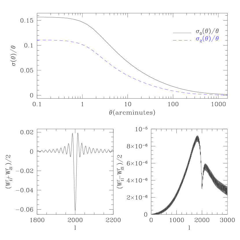
Figure 1 shows the functions that characterize the rms deflection of the photons, $\sigma_{0}(\theta)$ and $\sigma_{2}(\theta)$. On small scales the rms relative deflection between two photons approaches 15%, justifying the weak lensing assumption over most of the sky (for caustic formation one requires $\delta\theta\sim\theta$, which will occur only on rare occasions). We also show ${1\over 2}[{\cal W}_{1l}^{l^{\prime}}\pm{\cal W}_{2l}^{l^{\prime}}]$ for $l=2000$. The two window functions ${\cal W}_{1l}^{l^{\prime}}$ and ${\cal W}_{2l}^{l^{\prime}}$ are very similar, making their difference much smaller than their sum. One thus expects the generated $B$ type polarization from a pure $E$ type (and viceversa) to be very small. In fact ${\cal W}_{3l}^{l^{\prime}}$ is also very similar, the three windows only differ at the 1% level. The windows are oscillatory as a function of $l^{\prime}$ and their main contribution is concentrated around $l$.

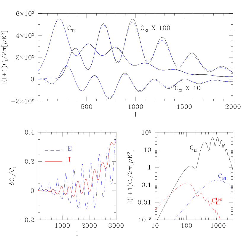
Figure 2 (upper panel) shows the lensed and unlensed power spectra. On intermediate scales lensing has the general effect of smearing the peaks in the spectrum by redistributing power. Polarization receives contribution only from velocity gradients at the last scattering surface and the acoustic peaks are very sharp. In contrast, temperature receives contributions both from velocity and density of photon-baryon plasma and the two are out of phase with each other, leading to a partial cancellation of acoustic peaks. One thus expects the effect of lensing to be larger for polarization and indeed we find that it is approximately a factor of two larger for $E$ polarization (figure 2, bottom left panel). In the damping tail the power is enhanced over the unlensed case as can be seen in the general trend in the relative difference between lensed and unlensed spectra (figure 2).

To asses the detectability of the induced $B$ polarization we will focus on the Plack mission. We assume that measurements of the temperature, $E$ type polarization and $T-E$ cross correlation have allowed the determination of the cosmological parameters accurately enough so that we know the approximate shape of the $B$ power spectra induced by lensing. We will attempt to determine just one parameter, the overall normalization of this $B$ signal, which expresses the overall effect of the matter fluctuations along the line of sight. If the signal to noise were large enough we could also attempt to determine the power spectrum of the lensing effect, by exploring the signal in $B$ as a function of $l$.

The relative error on the overall amplitude of the induced $B$ component $\beta$ is

$${\Delta\beta\over\beta}=\sqrt{2\over f_{sky}\sum_{l}(2l+1)/(1+w_{P}^{-1}B_{l}^{-2}/C_{Bl})^{2}};$$ (35)

$f_{sky}$ is the fraction of observed sky which we take to be $f_{sky}=0.8$. We assume the noise and beam width to be $w_{P}^{-1}=(0.025\ \mu K)^{2}$ and $B_{l}^{-2}=e^{l^{2}\sigma_{b}^{2}}$ with $\sigma_{b}=\theta_{fwhm}/2\sqrt{2\ln 2}=9\times 10^{-4}$. The effective number of modes contributing information is $N_{eff}=f_{sky}\sum_{l}(2l+1)/(1+w_{P}^{-1}B_{l}^{-2}/C_{Bl})^{2}$, so that $\Delta\beta/\beta=\sqrt{2/N_{eff}}$. For the experimental specifications above $N_{eff}\approx 8$ and $\Delta\beta/\beta\approx 0.5$. This means that there are only 8 independent modes of $B$ type polarization that can be observed with Planck, each a gaussian random variable with 0 mean and so the signal will be at the limit of detectability by Planck. The $B$ signal peaks at $l=1000$ and a ground based experiment observing a small patch of the sky for sufficiently long time to reduce the noise per pixel would be more effective to detect this signal. Gravitational lensing induced $B$ is also not a significant contaminant of the $B$ polarization expected from tensor modes in inflationary models [13], the latter being dominant on large angular scales (figure 2, bottom right panel, where we assumed tensors and scalars are of equal amplitude in the temperature on large scales).

FIG. 2.: The upper panel shows the $T$, $E$ and $C$ power spectra. Dashed (solid) lines correspond to the lensed (unlensed) spectra. The bottom left panel shows the relative difference between the lensed and unlensed spectra for $T$ and $E$ ($\delta C_{l}/C_{l}\equiv(C_{l}^{lensed}-C_{l}^{unlensed})/C_{l}^{unlensed}$) and shows both suppression of oscillations and enhancement of power on small scales. The bottom right panel shows the $B$ type polarization induced by lensing. We include the $E$ and $B$ spectra for inflationary model where scalars and tensors produce equal amount of power in the temperature on COBE scales ($T/S=1$).

IV Conlusions

The change in the CMB spectra induced by random deflections of the photons by the large scale structure of the universe has to be included in the calculations of the anisotropies when comparing theory and observations. We have presented a formalism to calculate the effect of gravitational lensing on all four CMB power spectra. The final expressions are given in a compact and numerically efficient form that is adequate for numerical implementation. These expressions have been implemented in the CMBFAST package, freely available from the authors. The computational time does not significantly increase with this feature and since the effect can be significant we feel the lensing effect should be included in any calculation where high precision accuracy is important, such as in the design and analysis of the CMB experiments. The method is self-consistent in the sense that for any cosmological model we use the actual power spectrum computed in the code to compute the lensing effect. The power spectrum is normalized to COBE using the CMB spectrum computed from the same code output. This approach gives the correct amplitude of gravitational lensing effect for the particular model in question. It should be pointed out that if the model is inconsistent with the small scale constraints such as $\sigma_{8}$ normalization then the amplitude of the lensing effect will also be incorrect. For example, COBE normalized standard CDM has a much larger gravitational lensing effect than what we find using the cosmic concordance model, but this is only a reflection of standard CDM model having too much small scale power to be compatible with small scale constraints. For models that are correctly normalized on small scales the relative change of the polarization power spectra can reach 10% at $l\sim 1000$ and even more at higher $l$. This is larger than in the temperature spectrum and is caused by the sharper acoustic peaks in the polarization spectra. In the damping region the lensed spectra show an enhancement above the unlensed spectra just like in the temperature case, although the sensitivity to this effect is too small for satellite missions to detect it in polarization [13].

Gravitational lensing also mixes $E$ and $B$ type polarization by deforming the polarization pattern on the sky relative to that at the last scattering surface. This will generate $B$ type polarization out of the $E$ type polarization even if there was no $B$ present at the last scattering surface. This induced $B$ mode is rather small in typical models and will be only marginally detectable by the Planck Surveyor. It peaks at fairly small angular scales around $l\sim 1000$ and so does not affect the measurement of gravity waves from $B$ polarization on larger scales. A ground based experiment observing a small patch of the sky would be more suitable to observe this effect and would allow one to determine the power spectrum of matter fluctuations. This would allow a detection of a combined gravitational effect from structures spanning a much larger range in redshift space than currently reachable by other methods.

REFERENCES

• [1] Jungman G., Kamionkowski M., Kosowsky A., and Spergel D. N. Phys. Rev. Lett., 76, 1007 (1996); ibid Phys. Rev. D 54, 1332 (1996); Bond J. R., Efstathiou G. & Tegmark M., MNRAS, 291, 33 (1997); Zaldarriaga M., Spergel D. N. and Seljak U. Astrophys. J. 488, 1 (1997)
• [2] Blanchard, A. and Schneider, J., Astron. & Astrophys. 184, 1 (1987); Cole, S. and Efstathiou, G., MNRAS 239, 195 (1989); CayΓ³n, L., MartΓ­nez-GonzΓ‘lez, E., & Sanz, J. L. Astrophys. J. 403, 471 (1993); ibid Astrophys. J. 489, 21 (1997)
• [3] Seljak U., Astrophys. J. 463, 1 (1996)
• [4] Metcalf, R. B., & Silk, J. Astrophys. J. 492, 1 (1998)
• [5] Seljak U. & Zaldarriaga M., Astrophys. J. 469, 437 (1996); M. Zaldarriaga, U. Seljak, & E. Bertschinger, Astrophys. J. 494, 491 (1998)
• [6] Surpi G. C. & Harari D. D., Report No. astro-ph/9709087
• [7] Seljak U., Astrophys. J. 482, 6 (1997)
• [8] Kamionkowski M., Kosowsky. A. and Stebbins, A., Phys. Rev. D 55, 7368 (1997)
• [9] Peacock, J. A. & Dodds, S. J., MNRAS 280, L19 (1996)
• [10] Bernardeau F., Astron. & Astrophys. 432, 15 (1997)
• [11] Zaldarriaga M., MIT Thesis (in preparation)
• [12] Ostriker, J. P. and Steinhardt, P. J., Nature, 377, 600 (1995)
• [13] Seljak, U. and Zaldarriaga, M., Phys. Rev. Lett., 78, 2054 (1997)