The Galactic globular cluster NGC 1851: its dynamical and evolutionary properties

Abstract

We have completely mapped the Galactic globular cluster NGC 1851 with large-field, ground-based $VI$ CCD photometry and pre-repair $HST$/WFPC1 data for the central region.

The photometric data set has allowed a $V$ vs. $(V-I)$ colour–magnitude diagram for $\sim$ 20500 stars to be constructed. From the apparent luminosity of the horizontal branch (HB) we derive a true distance modulus $(m-M)_{0}$ = 15.44 $\pm$ 0.20.

An accurate inspection of the cluster’s bright and blue objects confirms the presence of seven “supra-HB” stars, six of which are identified as evolved descendants from HB progenitors.

The HB morphology is found to be clearly bimodal, showing both a red clump and a blue tail, which are not compatible with standard evolutionary models. Synthetic Hertzsprung–Russell (HR) diagrams demonstrate that the problem could be solved by assuming a bimodal efficiency of the mass loss along the red giant branch (RGB). With the aid of Kolmogorov–Smirnov statistics we find evidence that the radial distribution of the blue HB stars is different from that of the red HB and subgiant branch (SGB) stars.

We give the first measurement of the mean absolute $I$ magnitude for 22 known RR Lyr variables ($<M_{I}({\rm RR})>=0.12\pm 0.20$ mag at a metallicity [Fe/H] = –1.28). The mean absolute $V$ magnitude is $<M_{V}(\rm RR)>=0.58\pm 0.20$ mag, and we confirm that these stars are brighter than those of the zero-age HB (ZAHB). Moreover, we found seven new RR Lyr candidates (six $ab$ type and one $c$ type). With these additional variables the ratio of the two types is now $N_{c}$/$N_{ab}=0.38$.

From a sample of 25 globular clusters a new calibration for $\Delta V_{\rm bump}^{\rm HB}$ as a function of cluster metallicity is derived. NGC 1851 follows this general trend fairly well. From a comparison with the theoretical models, we also find some evidence for an age–metallicity relation among globular clusters.

We identify 13 blue straggler stars, which do not show any sign of variability. The blue stragglers are less concentrated than the subgiant branch stars with similar magnitudes for $r>80$ arcsec.

Finally, a radial dependence of the luminosity function, a sign of mass segregation, is found. Transforming the luminosity function into a mass function (MF) and correcting for mass segregation by means of multi-mass King–Michie models, we find a global MF exponent $x_{0}=0.2\pm 0.3$.

1 Introduction

Galactic globular clusters (GGC) are dynamically evolved objects. In order to understand the interplay between the internal dynamical processes and the influence of the Galactic potential, we must study a sample of GGCs comprising objects whose concentration, position in the Galaxy, luminosity and metallicity cover the whole observed range. The mass function and the radial profile must be determined for each cluster, in order to carry out a detailed dynamical analysis.

The introduction of large-size CCDs has made this kind of investigations possible. With these detectors it is also possible to obtain deep photometry for the nearest globulars, and therefore to probe their mass functions over large mass intervals, in order to reach those MS stars which are more sensitive to dynamical effects (e.g. Pryor et al. 1986).

A rich sample of stars is also essential in order to reveal and study the shortest-lived (and hence poorly known) phases of the stellar evolution (Renzini & Buzzoni 1986). Furthermore, the interactions between the single stars affect their evolution (e.g. Djorgovski et al. 1991). To establish the reliability of the stellar evolutionary models, we must therefore ascertain to what extent a GC colour–magnitude diagram and luminosity function is changed by the interactions among its stars.

For the above reasons, our group started a project aimed at studying a number of globular clusters covering a wide range of the relevant parameters. NGC 1851 ($\alpha_{2000}=5^{\rm h}14^{\rm m}6^{\rm s}.30$; $\delta_{2000}=-40^{\circ}2\arcmin 50\farcs 00$) has been selected for its position and its concentration. Its galactocentric distance, which is about twice that of the Sun, and its distance of 7.1 kpc from the Galactic plane (Djorgovski 1993) make it a typical halo object. Its concentration $c=2.24$ is one of the highest in the list of Trager et al. (1995). A recent measurement of the cluster’s proper motion has confirmed that NGC 1851 has halo-type kinematics (Dinescu et al. 1996). According to these authors, the space velocities of the cluster are $U=256\pm 35$ km s^-1, $V=-195\pm 26$ km s^-1, $W=-122\pm 30$ km s^-1, $\Pi=195\pm 37$ km s^-1 and $\Theta=167\pm 37$ km s^-1.

Past photometric studies of the cluster are given in Alcaino (1969, 1971, 1976), Stetson (1981, hereafter S81), Sagar et al. (1988), Alcaino et al. (1990) and Walker (1992a, hereafter W92). The most exhaustive analysis is that of W92. His main results are that: (1) the cluster core, although unresolved, appears to be blue; (2) the HB is bimodal, showing both a red clump and an extended blue tail; (3) there are no radial trends in the relative numbers of red horizontal branch (RHB), blue horizontal branch (BHB) and red giant branch (RGB) stars for 48  $<r<$ 190 ; (4) the RGB “bump” is at $V$ = 16.15 $\pm$ 0.03 mag; (5) the population ratio $R=N({\rm HB})/N({\rm RGB})$ has a value 1.26 $\pm$ 0.10, which corresponds to a helium abundance $Y$ = 0.23 $\pm$ 0.01 (computed by means of the R-method; e.g. Renzini 1977); (6) there are six blue straggler (BS) stars and six supra-RHB stars $[$15.7 mag $<$ $V$ $<$ 16.0 mag; 0.6 $<(B-V)<$ 0.8$]$ in the region 120  $<r<$ 220 , and there is evidence of segregation only for the BS stars, so an origin for supra-RHB stars from BS stars is not supported by W92 data; (7) no significant abundance spread is found from the colour width of the main sequence (MS); and finally (8) an age of 14 $\pm$ 1 Gyr results from the $\Delta$ ($B$$-$$V$) method (Sarajedini & Demarque 1990; VandenBerg et al. 1990).

We have now obtained new large-field CCD $V$, $I$ photometry for NGC 1851. The new data set makes it possible to re-analyse the stellar content of the cluster with a much richer sample and, for the first time, allows a comprehensive study of its dynamical properties. However, the central regions of the cluster cannot be studied with this ground-based material, due to the extreme crowding of the core. To overcome this limitation, pre-repair Hubble Space Telescope (HST) images have been retrieved from the archives and reduced in order to sample the central stellar content, in particular the radial distribution of the HB stars. For the sake of comparison, the photometric catalogue of W92 has been also used.

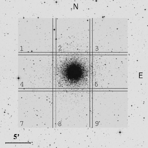
Figure 1: The observed NTT/EMMI fields, sketched over a POSS field.

Table 1: Log of NTT/EMMI observations.

Nr.	Field	$t_{\rm exp}$(s)	Filter	Date	FWHM $[\arcsec]$
1	6	50	$V$	1993 Feb 18	1.2
2	6	70	$I$	1993 Feb 18	1.2
3	5	45	$I$	1993 Feb 18	1.2
4	5	10	$I$	1993 Feb 18	1.4
5	5	10	$V$	1993 Feb 18	1.1
6	5	30	$V$	1993 Feb 18	1.3
7	2	30	$V$	1993 Feb 18	1.0
8	2	40	$I$	1993 Feb 18	1.2
9	3	60	$I$	1993 Feb 18	1.2
10	3	44	$V$	1993 Feb 18	1.1
11	1	45	$V$	1993 Feb 18	1.0
12	1	60	$I$	1993 Feb 18	1.2
13	4	60	$I$	1993 Feb 18	1.1
14	4	45	$V$	1993 Feb 18	1.1
15	7	45	$V$	1993 Feb 18	1.1
16	7	60	$I$	1993 Feb 18	1.2
17	8	70	$I$	1993 Feb 19	1.1
18	8	55	$V$	1993 Feb 19	1.1
19	9	55	$V$	1993 Feb 19	1.2
20	9	70	$I$	1993 Feb 19	1.2
21	back	120	$V$	1993 Dec 10	1.0
22	back	180	$I$	1993 Dec 10	1.1

2 The data set

Figure 2: The CMD from the NTT/EMMI data: stars with a daophot $\chi<1.5$ (Stetson 1987) are plotted. The 50 % completeness level and the saturation line are shown (dashed lines), The bright-blue supra-HB objects are marked with an asterisk.

The ground–based $V$, $I$ images have been obtained at ESO/La Silla with the 3.5 m New Technology Telescope (NTT) and the EMMI instrument at the Nasmyth focus. The list of the NTT/EMMI exposures is given in Table  1. Nine fields towards the cluster (1993 February) plus one background field (1993 December) have been observed, in moderate to good seeing conditions. The cluster fields cover a total area of 22 $\times$ 22 arcmin², which extends out to 1.3 tidal radii (cf. Sect. 5), and are sketched in Fig. 1.

Table 2: List of HST images.

Nr.	Date	Instr.	Filter	$t_{\rm exp}$(s)
1	1991 Feb 12	PC	F785LP	160
2	1991 Feb 12	PC	F555W	160

In order to complete the radial coverage, the $HST$ archives have also been scanned, and ten WFPC1 images of NGC 1851 were found. We reduced the two frames listed in Table 2, which have been taken in bands close to the $V$ and $I$ bands observed from the ground. These exposures cover the very centre of the cluster ($\sim$ 30${}^{\prime\prime}\times$ 30^′′).

A complete report of the reduction and calibration procedures is given in the Appendices, to which the reader is referred for details. We recall the main steps here. All frames have been pre-processed in the standard way, and the instrumental photometric catalogues have been obtained with the daophot+allstar (Stetson 1987) codes. Subsequent calibrations of the ground-based observations have been performed by means of five Landolt (1992) standard stars for the February run, plus eight standards for the December run. The HST CMD has been calibrated by comparison to the NTT/EMMI CMD (see Appendix B for more information). The overlap areas of the nine fields covering the cluster have been used in order to estimate the photometric zero-point accuracy (see Appendix A.2. for the details). Taking into account both internal and external errors, we estimate a zero–point error of 0.03 mag in the $V$ filter and 0.03 mag in the $I$ filter (1 sigma). The corresponding error in ($V$–$I$) is 0.04 mag. These figures apply also to the zero–points of the HST CMD.

Both completeness and the photometric errors have been evaluated with artificial star tests: the stars have been created with colours and luminosities representative of the MS–RGB sequence. The results of these tests are summarized in Table 11, which shows that the internal error keeps to within 0.1 mag until $V$ $\simeq$ 21 mag. A discussion of the completeness is deferred to Sect. 5 in the context of the analysis of the luminosity and mass functions.

3 The colour–magnitude diagram

Figure 3: The CMD of the background field. This is located at 30  east of the cluster centre and covers 9.6  $\times$ 7.4 . The solid line shows the fiducial points of NGC 1851, and stars within 2$\sigma$ of the line are further marked with open circles.

The calibrated CMD of NGC 1851 from the NTT data is presented in Fig. 2, while Fig. 3 shows the CMD of the background field. In order to better highlight the CMD features, only stars with allstar parameter $\chi$ $\leq$ 1.5 are plotted in Fig. 2 ($\simeq 20\,000$ stars). Here, the dashed lines mark the 50 % completeness level and the saturation limit: within these limits, the photometry extends from $\sim$ 1 mag below the RGB tip to $\sim$ 4 mag below the turn-off (TO). The richness of the sample allows the identification of the well populated main sequence, subgiant branch and giant branch, as well as the less represented horizontal branch, blue straggler sequence and asymptotic giant branch (actually, two AGBs can be seen in Fig. 2). In the following sections, we will carry out a detailed comparison of each sequence with current stellar models, and we first need to establish the cluster’s fundamental parameters: reddening, distance and metallicity.

3.1 Absolute calibration of the CMD

The most reliable estimate of the cluster reddening has been obtained by S81, using Strömgren photometry of the foreground stars. He determined $E_{B-V}$ = 0.02$\pm$0.01. A low value of the reddening is also to be expected considering the relatively great angular distance of NGC 1851 from the Galactic plane ($b=-35^{\circ}$): indeed, on the basis of the maps of Burstein & Heiles (1982), we would expect $E_{B-V}$ = $0.015\pm 0.02$. Therefore, we will adopt $E_{B-V}$ = 0.02; the extinction curve from Savage & Mathis (1979) then gives $A_{V}$ = 0.06, $E_{V-I}$ = 0.03 and $A_{I}$ = 0.03.

No direct estimates of the metallicity of NGC 1851 from high-dispersion spectroscopy exist. Current determinations are therefore based on a variety of spectroscopic and photometric metallicity indices, obtained both from integrated-light and single-star measurements. A brief account of recent determinations is now given.

Zinn (1980) measured the photometric metallicity index $Q_{39}$ from integrated spectra. By placing his sample of clusters on the high-dispersion metallicity scale of Cohen (1978a,b; 1979a,b) he obtained a value [Fe/H]$=-1.33$ from the NGC 1851 $Q_{39}$ value.

Frogel et al. (1983) obtained integrated infrared $(J-K)_{0}$ and $(V-K)_{0}$ colours of individual RGB stars of the cluster, which they used as metallicity indices calibrated on the new high–dispersion measurements of Cohen (1982, 1983). They estimated a metallicity [Fe/H]$=-1.26$.

Zinn & West (1984, ZW84) used the $Q_{39}$ value of Zinn (1980) and Cohen’s new metallicity scale to re-evaluate NGC 1851’s metallicity, which they found to be [Fe/H]$=-1.34\pm 0.09$.

Armandroff & Zinn (1988) measured the equivalent widths of the infrared Ca ii triplet on integrated spectra of the cluster. They used the scale of Zinn & West (1984) to rank their sample of clusters and obtained a value [Fe/H]$=-1.16$.

Da Costa & Armandroff (1995, DA95) repeated the measurement of the infrared equivalent widths, in this case using individual cluster RGB stars. These equivalent widths have recently been used by Rutledge et al. (1997) to obtain a new estimate of the cluster’s metallicity (DA95 used NGC 1851 as a calibration cluster). Depending on the method followed, Rutledge et al. find [Fe/H]$=-1.33\pm 0.09$ or $-1.23\pm 0.11$ if using the ZW84 scale, or [Fe/H]$=-1.03\pm 0.06$ on the Carretta & Gratton (1997, CG97) scale.

Taking the previous determinations as independent measurements of the NGC 1851 metallicity, we find a mean value [Fe/H]$=-1.28\pm 0.07$, obtained excluding the value on the CG97 scale. Using this datum we find [Fe/H]$=-1.24\pm 0.11$, which is entirely compatible with the previous value. On the other hand, until new consensus is reached on the CG97 scale, and for consistency with the other determinations the slightly higher value will be adopted in the following. We furthermore stress that our conclusions are by no means affected by the choice of either value.

Table 3: Summary of distance determinations.

Ref.	$V_{\rm HB}$	$A_{V}$	$M_{V}^{\rm HB}$	$(m-M)_{0}$
1	15.65	0.72	0.5	14.43
2	16.05 $\pm$ 0.1	0.06 $\pm$ 0.04	0.6	15.39 $\pm$ 0.23
3	16.05 $\pm$ 0.2	0.06	0.6	15.39 $\pm$ 0.20
4	15.80	0.42	0.5	14.88 $\pm$ 0.22
5	16.10	0.30	0.6	15.20
6	16.10	isochrone fit		15.45
1	Alcaino (1969)
2	Alcaino (1971)
3	Racine (1973)
4	Burstein & McDonald (1975)
5	Alcaino (1976)
6	Harris (1976)

Table 4: Data for the calculation of distance from HB luminosity: here $a$ and $b$ refer to the relation $M_{V}^{\rm HB}$ = $a$ [Fe/H] + $b$. We assume [Fe/H] = –1.28, $A_{V}$ = 0.06 and $V_{\rm HB}$ = 16.2 mag. An asterisk marks the data corrected as explained in the text.

Ref.	$a$	$b$	$M_{V}^{\rm HB}$	$(m-M)_{0}$
1	0.19	0.91	0.67	15.47
2	0.15	0.44	0.25	15.89
3	0.39	1.17	0.67	15.47
4	0.22	1.02	0.74	15.40 (*)
5	0.20	1.21	0.95	15.19
6	0.20	0.93	0.67	15.47 (*)
7	0.51	1.58	0.93	15.21
1	Rood & Crocker (1989): theoretical
2	Fusi Pecci et al. (1990): RGB bump
3	Sandage & Cacciari (1990): period-shift
4	Lee et al. (1990): theoretical
5	Carney et al. (1992): Baade–Wesselink
6	Walker (1992b): LMC Cepheids + RR Lyr
7	Rees (1993): statistical parallaxes

The previous distance determinations for NGC 1851 are less than satisfactory. Indeed, Table 3 shows the distance moduli available in the literature: they range from $(m-M)_{0}=14.43$ (Alcaino 1969) to $(m-M)_{0}=15.45$ (Alcaino et al. 1990), with $<(m-M)_{0}>=15.12\pm 0.36$.

Almost all the above determinations of the distance (cf. Table 3) are based on the luminosity of the HB compared to its absolute luminosity, where the latter is assumed not to vary with metallicity. Here we re-evaluate the distance allowing the absolute visual magnitude of the ZAHB, to vary with the metal content according to the law

$M_{V}^{\rm ZAHB}$ = $a$ [Fe/H] + $b$,

where the values of the parameters $a$ and $b$ are still controversial. Table 4 shows some recent determinations of these parameters. Accordingly, the distance modulus has been computed adopting, from the previous discussion, [Fe/H] = –1.28 and $A_{V}$ = 0.06.

The peak in the $V$ distribution of the HB stars is at $V$ = 16.2 $\pm$ 0.20 mag (see Fig. 2). Since the number of stars in a region of the CMD is proportional to the lifetime of the corresponding evolutionary phase, the stars belonging to this peak must be identified with the longest-lived phase of an HB star, which corresponds to a region close to the ZAHB. We note that the relation reported in Table 4 should strictly hold for ZAHB stars. In those cases in which the authors give a relation for RR Lyr stars, the coefficients were corrected following Carney et al. (1992), who find:

$M_{V}^{\rm RR}$ = $M_{V}^{\rm ZAHB}$ – 0.05 [Fe/H] – 0.20

(see also Catelan 1992). Corrected data are marked with an asterisk in Table 4. A mean of the listed moduli gives $(m-M)_{0}$ = 15.44 $\pm$ 0.20, which also results from the isochrone fitting (see below). This is the distance modulus we will adopt in the following.

3.2 Main sequence and red giant branch

Table 5: Fiducial points and widths along the MS–SGB–RGB sequence.

$V$ range		$<V$–$I>$	$\sigma$	$(V-I)_{\rm max}$	Bin
15.50	15.75	1.03	0.03	1.02	0.02
15.75	16.00	1.01	0.02	1.02	0.02
16.00	16.25	0.99	0.02	1.00	0.02
16.25	16.50	0.98	0.03	0.98	0.02
16.50	16.75	0.94	0.02	0.94	0.02
16.75	17.00	0.95	0.02	0.94	0.02
17.00	17.25	0.92	0.02	0.92	0.02
17.25	17.50	0.90	0.03	0.90	0.02
17.50	17.75	0.90	0.03	0.90	0.02
17.75	18.00	0.88	0.03	0.88	0.02
18.00	18.25	0.89	0.03	0.90	0.02
18.25	18.50	0.86	0.03	0.86	0.02
18.50	18.75	0.85	0.03	0.84	0.02
19.00	19.25	0.70	0.08	0.67	0.03
19.25	19.50	0.68	0.07	0.68	0.02
19.50	19.75	0.68	0.07	0.67	0.03
19.75	20.00	0.68	0.06	0.66	0.02
20.00	20.25	0.71	0.07	0.70	0.03
20.25	20.50	0.72	0.08	0.72	0.04
20.50	20.75	0.76	0.09	0.76	0.04
20.75	21.00	0.77	0.10	0.75	0.05
21.00	21.25	0.83	0.13	0.85	0.05
21.25	21.50	0.87	0.15	0.88	0.06
21.50	21.75	0.90	0.15	0.88	0.06
21.75	22.00	0.95	0.18	0.94	0.07
22.00	22.25	1.02	0.18	1.04	0.08
22.25	22.50	1.04	0.18	1.04	0.08
22.50	22.75	1.15	0.21	1.12	0.08
22.75	23.00	1.28	0.26	1.33	0.09
Turn-off
$V$–$I$ range		$<$$V$$>$	$\sigma$	$V_{\rm max}$	Bin
0.65	0.70	19.26	0.17	19.20	0.15
0.70	0.75	19.13	0.15	19.20	0.15
0.75	0.80	19.03	0.13	19.00	0.10
0.80	0.85	18.82	0.11	18.80	0.10
0.85	0.90	18.62	0.23	18.60	0.20

In order to establish our fiducial lines and to compare the observed widths with the photometric errors, a careful analysis of the colour distribution along the MS–SGB–RGB sequence has been made. We assumed a Gaussian colour distribution and determined the mean colour and dispersion, $\sigma$, in each magnitude interval: these data are grouped in Table 5, where the mode of the distribution and the bin width (1 $\sigma$) are also listed.

Once the observed widths of Table 5 are compared with the $\sigma$ associated with the photometric errors (Table 11), it can be seen that the former are compatible with a null intrinsic colour dispersion along the MS–SGB–RGB sequence that translates into a null dispersion in metallicity (see e.g. Renzini & Fusi Pecci 1988).

3.3 The RGB bump

Figure 4: Luminosity function (LF) for the evolved stars in NGC 1851: the differential LF is shown in the upper panel; the cumulative LF is plotted in the lower panel. The bump in the LF is clearly seen in both the differential and cumulative LF at $V$ = 16.15 $\pm 0.15$ mag.

Figure 5: The quantity $\Delta V_{\rm bump}^{\rm HB}$ as a function of the parameter $s(Z)$ = sinh^-1 ($Z_{4}$/2.5) (see text); a linear fit to the data yields $\Delta V_{\rm bump}^{\rm HB}$ = 0.33 $s(Z)-0.70$ (0.06 rms). The filled triangle represents NGC 1851 and the open triangles represent M 80, M 4 and NGC 6352 (Saviane & Piotto in prep.); the open circles are the original sample of Fusi Pecci et al. (1990) and the open squares are 3 other clusters from Sarajedini & Norris (1994). Also represented are the linear fit (solid line) and the theoretical relations from Bertelli et al. (1994, dashed line) and Rood & Crocker (1989, dotted line).

The RGB bump was first predicted by Iben (1968) in the evolutionary phase of H-burning in a shell: the bump is located on the RGB at a luminosity which depends on the metallicity and on the age of the cluster, and generally speaking it is not a prominent feature. For example, Iben (1968) predicted that the ratio of lifetimes between the bump and the HB phases is $t_{\rm bump}/t_{\rm HB}=0.025$ and that the ratio between the bump and RGB phases is $t_{\rm bump}/t_{\rm RGB}=0.035$ for $Y=0.35$ and $Z=2\cdot 10^{-4}$; therefore, for every 100 RGB stars just $\sim 4$ will be found in the bump (slightly higher figures are obtained for lower $Y$ values). Moreover, in metal-poor clusters the bump is located in the bright part of the RGB, where the statistics are poor and it can be lost in the count noise. For this reason, it has not been detected until recently (King et al. 1985). Afterwards, it has been studied on a sample of GCs by Fusi Pecci et al. (1990, FP90), and the sample has been further extended by Sarajedini & Norris (1994). As shown in Fig. 4, the bump in the RGB of NGC 1851 is located at $V$ = 16.15 $\pm$ 0.15 mag. Assuming $V_{\rm HB}$ = 16.20 $\pm$ 0.03 mag (cf. Sect. 3.1) we have obtained $\Delta V_{\rm bump}^{\rm HB}=-0.05\pm 0.15$.

FP90 provide a relative calibration for $\Delta V_{\rm bump}^{\rm HB}$ which corresponds to the difference between the absolute magnitude of the bump ($M_{V}^{\rm bump}$) with respect to the luminosity of the HB ($M_{V}^{\rm HB}$), for a sample of 11 globular clusters. The value determined for NGC 1851 is in good agreement with the above calibration. In fact, we have extended this calibration with the inclusion of seven additional clusters from Sarajedini & Norris (1994, three clusters), Saviane & Piotto (in prep., three clusters) and NGC 1851 (this paper). We find that the best fit is given by the following relation:

$$\Delta V_{\rm bump}^{\rm HB}=0.33\sinh^{-1}\left(\frac{Z_{4}}{2.5}\right)-0.70\,\,\,(0.06\,\,{\rm rms}).$$

The parameter sinh^-1 ($Z_{4}$/2.5) is chosen in order to linearize the dependence on the metallicity; $Z_{4}$ is the metallicity in units of 0.0004. Since the dependence of the luminosity of the HB on [Fe/H] accounts only for a variation of 0.3–0.4 mag in $\Delta V_{\rm bump}^{\rm HB}$ in the metallicity interval covered by our data, Fig. 5 shows that the bump goes fainter when higher [Fe/H] values are considered. It is also evident that NGC 1851 (filled triangle) follows the general trend.

As far as the theoretical interpretation is concerned, we first considered the canonical models by Rood & Crocker (1989) whose relation is given in FP90 assuming a constant age (15 Gyr) and helium abundance ($Y=0.23$). In Fig. 5 this relation is shown as a dotted line, and it can be seen that its slope is similar to the observational one, but there is a clear luminosity difference, in the sense that the theoretical values are brighter than the empirical ones ($\sim 0.4$ mag for the lower metallicities and $\sim 0.5$ mag for the higher ones). Some attempts to solve this problem are examined below.

On the basis of spectroscopic observations of giant stars in globular clusters (e.g. Gratton & Ortolani 1989), which show that in these stars the $\alpha$ elements are enhanced with respect to the solar values, Salaris et al. (1993) presented Population II isochrones computed with such non–standard chemical compositions. One of the main properties of $\alpha$-enhanced isochrones is that they are well reproduced by solar-scaled isochrones. If we take an isochrone of metallicity $Z_{0}$ whose $\alpha$-elements are enhanced by a factor $f$, it can be represented by a solar-scaled isochrone of a higher metallicity $Z=Z_{0}\,(0.638\,f+0.362)$. A solar-scaled isochrone is one with solar metallic partition and scaled in global metallicity from $Z_{0}$ (that of the alpha-enhanced metallic partition) to $Z$, according to the above formula. Straniero et al. (1992) suggest that these kinds of models could solve the RGB bump discrepancy, since a higher metallicity would make the bump fainter and therefore $\Delta V_{\rm HB}^{\rm bump}$ fainter as well.

In order to quantify this effect, we can use the observed relation $\Delta V_{\rm HB}^{\rm bump}$ vs. [Fe/H]. Even if it is not exactly linear, a good approximation is $\Delta V_{\rm HB}^{\rm bump}=0.66$ [Fe/H]$+0.87$. The relation between $Z$ and $Z_{0}$ can be transformed into [Fe/H] $\simeq$ [Fe/H]${}_{0}-\log(0.638\,f+0.362)$. All current estimates give an upper limit of $f\simeq 4$ (see the compilation in Salaris et al. 1993), and even adopting this extreme value we find that the theoretical $\Delta V_{\rm HB}^{\rm bump}$ can be made only $\simeq$0.3 mag fainter.

Another approach is to consider that a certain amount of convective overshoot occurs at the bottom of the envelope of low-mass stars while climbing the RGB (King et al. 1985; Alongi et al. 1991). In this set of models the envelope goes deeper into the innermost nuclear processed regions of the star, hence the first dredge-up is anticipated. As a consequence, the bump is moved $\sim$ 0.4 mag fainter. The isochrone library by Bertelli et al. (1994) assembles stellar models adopting this prescription and the dashed line in Fig. 5 shows the resulting fairly good agreement with the observed luminosities in the metal range covered. As for the relation labelled “Rood & Crocker 1989” in Fig. 5, also the relation labelled “Bertelli et al. 1994” has been derived assuming a constant age of 15 Gyr. The helium content is not constant but follows the ratio $\Delta Y/\Delta Z=2.5$. This means higher helium content for metal-rich clusters.

We note a possible residual offset at the high- and low-metallicity ends between the data and the Bertelli et al. (1994) relation, specifically the theoretical relation seems to predict lower values for $\Delta V_{\rm HB}^{\rm bump}$ at $s(Z)<2.2$ and higher values at $s(Z)>2.2$. The discrepancy depends either on the HB or on the bump luminosities. In the first case, Fig. 5 shows that the HB luminosity is too high for metal-rich clusters, and too low for metal-poor ones. Conversely, in the second case the bump occurs at luminosities that are too low for the metal-rich clusters and too high for the metal-poor ones.

The HB luminosity is mostly controlled, at fixed metallicity, by the helium content. Higher $Y$ means brighter HB luminosities. A different (lower) $\Delta Y/\Delta Z$ ratio would act in the right direction, lowering the HB luminosity at high $Z$ values and enhancing it at low $Z$ values.

It should also be remembered that the luminosity of the RGB bump critically depends, at fixed metallicity, on the age. Specifically, lower ages imply higher RGB stellar masses which in turn possess higher luminosities. As a consequence, an interesting way of removing the cited offsets would be to assume that high-metallicity clusters are younger than low-metallicity ones. To quantify the required corrections, we computed values for the age differences at the extremes of the metallicity range covered by the models. We found that for [Fe/H] = –0.4 the clusters should have an age $\simeq 3.3$ Gyr lower and for [Fe/H] = –1.74 they should have an age $\simeq 1.6$ Gyr higher than the age of metal-intermediate clusters. The present comparison would therefore suggest an age-metallicity relation among globular clusters, with an age difference of $\simeq 5$ Gyr between metal-poor and metal-rich objects. However, we caution the reader that in any case the uncorrected relation is fairly compatible with the observations given the associated errors, and the quoted age difference could be considered as an upper limit. In summary, we argue that both $\alpha$-enhanced chemical composition and envelope overshoot could actually exist in real GC stars. The former is observational evidence, but even considering this effect in theoretical models, the discrepancy seems to be not completely removed, thus some degree of overshoot must be invoked. Therefore, the suggested age-metallicity relation should be more carefully probed with improved models including both effects.

3.4 AGB and supra horizontal branch stars

Figure 6: Enlarged portion of the CMD showing in better detail the horizontal branch region. Stars brighter than the HB and bluer than the AGB are marked with an asterisk and numbered (supra-HB stars). The solid lines are the “planetary nebula” part of two isochrones, computed for an age of 15 Gyr and two different mass losses along the RGB (see text). The other lines correspond to the tracks of stars evolving off-HB, for different initial HB masses and compositions ($Z$=0.001 for the dotted lines and $Z$=0.0004 for the dashed lines). Going from bluer to redder colours the initial HB masses are 0.50, 0.52 and 0.55 $M_{\odot}$ for the lower metal content, and 0.60, 0.65 and 0.70 $M_{\odot}$ for the higher metallicity. The $V$ magnitude of the plateau of the post-HB tracks is roughly the same for the two adopted metallicities. The majority of supra-HB stars can be identified with some post-HB evolutionary phase.

A number of stars are found in the CMD area brighter than the HB and bluer than the AGB (the so-called “supra-HB” stars), and in Fig. 8 (upper panel) a dotted line marks the limit of what we considered supra-HB candidates, namely stars 1 mag brighter than the HB and bluer than the AGB. We have found $\sim$ 50 stars in this region. They have been inspected on the original frames and catalogued according to (a) the allstar photometric parameters, (b) the product and the ratio of the FWHM and (c) the value of the brightest pixels. 17 stars are found to have some saturated pixels in the I filter, and 16 more are blends (the product of the FWHMs is more than 2 times the mean one, or the sum of the $\chi$ parameters is greater than 10). Of the remaining group, 7 stars have a sum of the daophot $\chi$ in the two filters less than 4, and therefore can be considered objects with good photometry, while the remaining 11 stars, with 4 $<$ $\chi$ $<$ 10, are probable blends and hence discarded. The seven objects which passed this selection are marked with an asterisk in Fig. 2; they present normal star-like shape, do not have saturated pixels and are not in blends.

From Fig. 3 we see that hardly any field stars are expected in this CMD area, and indeed the Bahcall & Soneira model (Bahcall 1986; adapted to the ($V$–$I$) colour as in Saviane et al. 1996) predicts at most 1 star for a colour range ($V$–$I$) $<$ 0.5, within an area of 484 arcmin² in the direction $l=244^{\circ}$, $b=-35^{\circ}0$; thus, most of the supra-HB objects are likely stars of the cluster. In order to identify their evolutionary status, we plotted in Fig. 6 an enlargement of the HB region where supra-HB stars have been numbered, and a number of isochrones and tracks superimposed. The dotted lines represent the post-HB evolutionary tracks for initial HB masses 0.60, 0.65 and 0.70 $M_{\odot}$ taken from the Padua library with $Z$=0.001. The theoretical plane has been translated into the observational one through the library of stellar spectra by Kurucz (1992). These tracks are able to explain the evolution of HB and later phases for stars on the blue tail (0.6 $M_{\odot}$ tracks), intermediate HB (0.65 $M_{\odot}$) and red HB (0.7 $M_{\odot}$), and to partially reproduce the observed dispersion in colour along the AGB. This range of masses is larger than what one would expect from normal mass-loss rates and their dispersion along the RGB. A deeper analysis of this subject is given in Sect. 4.

Since the library we are using does not contain models for HB masses lower than 0.6 $M_{\odot}$ and $Z$=0.001, the evolution of smaller HB masses can be explored by using the $Z$=0.0004 models and the bolometric corrections pertaining to them, even if this value of $Z$ is less than the assumed cluster metallicity. In fact, comparing the 0.6 $M_{\odot}$ tracks for the two metallicities we verified that their differences in effective temperatures and luminosities are not dramatic. On the other hand, when applying the bolometric corrections, we find that the 0.06 dex difference in the ZAHB $\log T_{\rm eff}$ implies that the $Z$=0.001 model starts $\sim 0.4$ $V$ mag brighter than the Z=0.0004 model, while the absolute V magnitude of the post-HB “plateau” is roughly unchanged. Therefore, the reader should not give too much importance to the fact that in Fig. 6 the lower–mass evolutionary tracks start in an HB region almost devoid of stars. There are in fact two effects that should be taken into account. First, a choice of the correct metallicity would make the HB starting point brighter; secondly, theoretical bolometric corrections could be slightly overestimated at these temperatures.

These lower-metallicity tracks (dashed lines in Fig. 6) are for initial HB masses 0.50, 0.52 and 0.55 $M_{\odot}$, going from the bluer to the redder one. We first note that this set of $M<0.6\,M_{\odot}$ tracks is able to reproduce the bluer AGB, which is seen as a separate branch running parallel to the higher-mass AGB, already discussed (see Fig. 6). It is also evident that the location of stars 4 and 5 is compatible with the 0.52 $M_{\odot}$ track, in the post-HB phase approaching the AGB. Furthermore, we notice that (a) the post-HB evolution of the 0.50 $M_{\odot}$ model is quite different from that of the 0.52 $M_{\odot}$ one, and (b) a decrement in mass as small as 0.03 $M_{\odot}$ between the two redder models increases their post-HB luminosity by $\sim 1$ mag. The 0.50 $M_{\odot}$ model evolves directly from the HB to the planetary nebula (PN) regime, skipping the AGB phase (AGB-manqué; e.g. Fagotto et al. 1994 and references therein). In the cited mass interval we therefore expect that, for decreasing masses, a brighter and brighter post-HB phase will be reached, until the star envelope is so much reduced that the AGB cannot be developed. From this point on, the resulting AGB-manqué phase will attain lower and lower luminosities. On the basis of these arguments, it is possible that a model with initial HB mass $0.50\ M_{\odot}<M<0.52\ M_{\odot}$ be able to develop the AGB after passing a post-HB phase as luminous as the level of stars 6 and 7.

Instead, stars 2 and 3 can be identified as objects in the PN phase either evolving from the classical post-AGB or in the final AGB-manqué phase. The first case is shown by the solid lines in Fig. 6, which are the PN portion of two isochrones, computed for an age of 15 Gyr and a RGB mass-loss efficiency in the Reimers formalism $\eta=0.25$ (the brighter one) and $\eta=0.43$ (the fainter one). These efficiencies have been chosen after the analysis in Sect. 4, and represent the reasonable boundaries which are required in order to explain the blue and red part of the HB. The corresponding core masses, $M_{\rm c}$, for the two PNe are $M_{\rm c}=0.581\,M_{\odot}$ and $M_{\rm c}=0.537\,M_{\odot}$. The second case would be given by a track similar to the 0.50 $M_{\odot}$, $Z$=0.0004 model with a slightly higher initial HB mass.

Star 1 seems not to be compatible with either of the above predictions, since its ($V$–$I$) colour ($\simeq-0.5$) is bluer than that of the maximum blue excursion of PNe, which are the bluest objects expected for this cluster. There is a remote possibility that star 1 is a foreground object. Its colour is compatible with extreme values that are observed for field stars. For example, the catalogue of Landolt (1992), contains two objects (SA 107 215 and PG 0231 051), whose ($V$–$I$) colours ( –0.511 and –0.534, respectively) are of the same order of the one of star 1. The presence of 1 star in this CMD area is in agreement with the field-star contamination previously evaluated.

A further test giving clues on the nature of the supra-HB stars, would be to compare the relative counts of HB and post-HB objects to those observed in globular clusters. However, in our case this test is not significant. In fact, we estimated the ratio $N$(post-HB)/ $N({\rm HB})$ to be $0.18\pm 0.04$, which is compatible with the ratio $R_{2}=N({\rm AGB})/N({\rm HB})=0.15\pm 0.05$ (Buzzoni et al. 1983) determined on a sample of GCs. Excluding the seven supra-HB stars, our ratio is only slightly lowered and hence still compatible with the observed $R_{2}$.

Finally, if supra-HB stars are the descendants of HB stars we also expect them to follow the same radial distribution. Unfortunately, there are too few supra-HB stars in our sample to do any statistical test, while they are saturated in the HST/WFPC1 images.

3.5 RR Lyrae stars

Table 6: Positions and photometry of RR Lyrae stars. The variable type ($ab$ or $c$) is taken from the references numbered as follows: (1) Liller (1975), (2) Wehlau et al. (1978) and (3) Wehlau et al. (1982). Other characteristics taken from these references are labelled “n”, “bl.”, “lP”, “fld” indicating, respectively, non-variable, blend, long period and field star. Star 24 has a possible period of 183 days and is labelled “183”.

$N$	$x^{\prime\prime}$	$y^{\prime\prime}$	$\Delta x$	$\Delta y$	$I$	$(V$–$I$)	Type/ref
1	257.9	–11.4	0.6	–0.9	15.56	0.54	ab 2
2	–40.5	29.3	–0.8	0.9	15.22	0.97	n,bl. 1,2
3	–42.6	94.4	0.6	0.6	15.61	0.32	c 2
4	25.7	35.6	–1.0	0.2	15.88	0.67	ab 2
5	41.3	40.2	0.0	1.0	15.35	0.49	ab 2
6	–74.0	–8.3	–0.3	0.1	15.81	0.68	ab 2
7	3.4	–110.2	–0.4	0.2	15.45	0.49	ab 2
8	29.6	25.5	–0.7	–0.8	15.60	0.49	ab 2
9	–56.7	49.5	–1.1	0.0	13.59	0.24	lP,n 1,2
10	45.6	–197.4	1.2	0.8	15.90	0.60	ab 2
11	67.0	–136.8	–1.0	–0.2	15.72	0.66	ab 2
12	–77.2	–45.9	0.2	–0.1	15.32	0.35	ab 2
13	5.4	45.9	0.6	0.1	15.70	0.20	c 2
14	74.6	16.1	0.4	–0.1	14.85	0.60	ab 2
15	32.5	51.2	–0.5	–0.2	15.49	0.51	ab 2
16	67.3	–0.7	–0.3	–0.3	15.98	0.45	ab 2
17	–42.2	–55.5	0.2	0.5	15.55	0.66	ab 2
18	45.5	158.7	0.5	0.3	15.75	0.32	c 2
19	26.0	–32.6	–1.0	–0.4	15.67	0.43	c 2
20	–10.5	–23.0	0.5	0.0	15.69	0.57	ab 2
21	–58.7	61.8	–0.3	0.2	15.90	0.28	c 2
22	131.0	108.7	0.0	–0.7	15.47	0.55	ab, bl. 3
23	110.0	–57.6	–1.0	–0.4	15.78	0.23	c 3
24	144.5	–96.5	saturated				183? 3
25	–131.1	–274.6	2.1	0.6	14.86	0.79	c 3
26	–123.9	106.7	–0.1	0.3	15.68	0.41	fld. 3
99	–84.4	106.2	0.4	–0.2	15.51	0.63	n 3

Extensive studies of NGC 1851 variables are found in Liller (1975), Wehlau et al. (1978, WLDC) and Wehlau et al. (1982); on the basis of the value $N_{c}$/$N_{ab}$ = 0.47, the cluster has been classified as Oosterhoff type I.

Using the RR Lyr coordinates given by these authors and by Fourcade & Laborde (1966), our catalogue has been searched in order to identify the variables. Twenty-six out of 27 variable stars have been successfully found, and these are reported in Table 6: in this table, $N$ is the identification number used in the literature, $x$ and $y$ are the coordinates of our stars (in arcsec) and “type” is the RR Lyr type given by Wehlau et al. (1978, 1982) and Liller (1975). The frame of reference is centered at ($\alpha$,$\delta$; eq.) = (5^h 12^m.4, –40^∘ 05^′; B1950.0). The transformation from our frame of reference to WLDC is:

$$\left\{\begin{array}[]{ll}x_{\rm W}=-528.6+x+0.0179\cdot y\\ y_{\rm W}=-499.1-0.0179\cdot x+y\end{array}\right.$$

There is a rotation angle of $\simeq$ 1.03 deg; also, the scale factor 0.44 must be applied to $x_{\rm W}$ and $y_{\rm W}$; the residuals $\Delta x$ and $\Delta y$ in the coordinates after the transformation are also reported in Table 6. Column 6 and 7 of Table 6 give our determination of $I$ and ($V$–$I$); the mean magnitudes, colours, and periods of these RR Lyr are listed in WLDC78 and Wehlau et al. (1982). In this table, actually 22 are true RR Lyr variables (15 ab and 7 c type); stars 2, 9 and 99 are thought to be non–variables (and actually do not scatter in Fig. 17), star 26 could be a W UMa field star, and finally star 24 could be a long–period variable. This latter star has not been measured because it is located at the RGB tip (cf. W92), and is saturated in our images. Star 9 is a very red star below the RGB tip: it is almost saturated in $I$, so it has an artificially blue colour and for this reason it has not been plotted in our CMD.

Our photometry of the RR Lyr in Table 6 gives a mean magnitude $<$V$>_{\rm RR}$ = 16.08 $\pm$ 0.06 mag, where the error reflects the intrinsic dispersion of their distribution, which corresponds to $<M_{V}({\rm RR})>=0.58\pm 0.20$ mag with the assumed distance modulus and absorption (Sect. 3.1). Therefore, RR Lyr stars are 0.12 mag brighter than the ZAHB at $V_{\rm HB}=16.2\pm 0.03$ mag (cf. Sect. 3.1). Using the relation of Carney et al. (1992) a value $<$V$>_{\rm RR}$ = 16.11 mag is predicted, well inside the 1-sigma uncertainty. The internal uncertainty in the RR Lyr colours can be estimated from Table 11, which gives $\leq$0.04 mag for $V$$<$16.74 mag. Adding the calibration uncertainty, we obtain a total error of 0.06 mag. Finally, we can also give for the first time the mean $I$ magnitude of the RR Lyraes: we find $<$$I$$>_{\rm RR}$ = 15.59 $\pm$ 0.06 mag, corresponding to $<M_{I}({\rm RR})>=0.12\pm 0.20$ mag, assuming $A_{I}=0.03$ and $(m-M)=15.44\pm 0.2$.

3.6 New RR Lyrae candidates

Figure 7: The location of known and suspected variables in the NGC 1851 CMD: the different symbols refer to RR Lyr stars (crosses), the candidate RR Lyraes (full dots), and (c) other blue objects (open triangles) and red objects (open squares and filled squares) which are discussed in Appendix A.2. Also plotted are the blue straggler stars (open dots): these stars are fainter than the limit imposed by a 2 Gyr, $Z$=0.001 isochrone (dotted line), which has a TO mass $m_{\rm TO}\simeq 1.5\,M_{\odot}$. The solid line represents the fiducial sequence of NGC 1851 and the horizontal dotted line represents the fainter limit of the W92 photometry. See also discussion in Appendix A.2.

Table 7: Positions and photometry of variable candidates.

$n$	$x^{\prime\prime}$	$y^{\prime\prime}$	$V$	($V$–$I$)	$\Delta V_{\rm W}$	$\Delta V_{\rm RR}$	Type
1	–38.5	–28.8	15.39	0.76	–0.23	–0.66	ab
2	–9.2	32.9	16.22	0.64	0.38	0.17	ab
3	–31.6	–11.0	16.37	0.65	0.35	0.32	ab
4	–18.9	38.1	16.21	0.71	0.15	0.16	ab
5	–15.6	–17.8	15.91	0.78	–0.18	–0.14	ab
6	–5.2	–53.1	15.97	0.44	–0.35	–0.08	c
7	–12.1	–20.2	16.19	0.86	–0.14	0.14	ab

When our photometry is compared with that of W92, it can be seen (Fig. 17) that a number of stars at the level of the HB are located outside the “3-$\sigma$” lines. These stars have been extracted from the photometric catalogue and inspected both on the $V$ and $I$ images, in order to remove non-stellar objects. A “quality” parameter has been devised, including remarks about the FWHM, the presence of neighbours, the shape and the blending: the stars that passed these criteria are listed in Table 7. From left to right, the columns report an identification number, the coordinates in the WLDC frame of reference, the magnitude and colour in our photometry, the magnitude difference with respect to the W92 values and the mean RR Lyr value, and finally the estimated variable type. These stars are also plotted in Fig. 7, where different symbols are used to identify (a) the known RR Lyr stars (crosses) discussed in the previous section and (b) the new RR Lyr candidates (full dots).

From the location in Fig. 7, six of the seven RR Lyr candidates can be assigned to the $ab$ type and one to the $c$ type: this would bring the ratio $N_{c}$/$N_{ab}$ to the value $0.38\pm 0.22$, in better agreement with the value found for the other clusters of comparable metallicity. In fact, the catalogue of Castellani & Quarta (1987) can be used to calculate the expected $N_{\rm c}$/$N_{\rm ab}$ ratio. There are six clusters with [Fe/H]$\sim-1.3$ in the compilation. If we exclude NGC 1851 itself, NGC 362 (which has no $c$ type RR Lyr) and NGC 6864 (which has only six variables, whose ratio also happens to be too uncertain), a weighted mean of the three remaining clusters yields a value $N_{\rm c}$/$N_{\rm ab}=0.23\pm 0.09$. For comparison, Smith (1995) gives a value $N_{\rm c}$/$N_{\rm ab}=0.20$ as representative of the Oo I clusters. The ratio of NGC 1851 is therefore 2.6 sigma higher than the value found for the clusters of similar metallicity.

A determination of the light curves for the candidate variables is required in order to confirm this result in the N_c/N_ab ratio of the RR Lyr variables in NGC 1851.

3.7 The blue straggler stars

Table 8: Coordinates and photometry of the candidate blue straggler stars. The $x$ and $y$ data are expressed in arcsec in the Wehlau et al. (1978) frame of reference.

$N$	$x^{\prime\prime}$	$y^{\prime\prime}$	($V$–$I$)	$V$
1	107.4	–194.0	0.13	17.60
2	–124.9	2.6	0.38	18.31
3	–156.6	114.6	0.46	18.95
4	–110.6	127.7	0.23	18.40
5	186.7	189.8	0.54	18.59
6	131.9	194.3	0.25	18.63
7	–83.1	–152.8	0.34	18.11
8	160.9	–46.6	0.36	18.70
9	222.4	44.8	0.56	18.72
10	6.5	–164.0	0.49	19.13
11	243.1	93.6	0.26	18.54
12	–132.1	427.8	0.24	17.87
13	–292.2	–148.9	0.48	19.12

Thirteen blue straggler stars have been identified in the photometric catalogue in the region $r>80$ arcsec (the crowding did not allow a clear identification of BS stars closer to the cluster center) and they are listed in Table 8. The columns are, from left to right, the identification number, the positions in the WLDC frame of reference, the colour and magnitude in our photometric system.

Blue straggler stars are objects which are located in the region between the TO and the blue tail of the HB and are distributed along a sequence normally filled by MS stars younger than those of a GC. Bolte et al. (1993) and Ferraro et al. (1995), among others, have studied the BS stars frequency in GGCs, and Ferraro et al. (1995) found that clusters which are more massive and denser have more BS stars with respect to clusters of lower mass and density.

BSs are thought to be the result of the merging (by coalescence of binaries or collision) of two main-sequence stars. If we define $m_{\rm BSS}$ the mass of any BS stars and $m_{\rm TO}$ the mass of a TO star, it should always be $m_{\rm BSS}<2\,m_{\rm TO}$. The BS star sample in NGC 1851 is compatible with this statement, as can be seen in Fig. 7: all the 13 identified BS stars are less luminous than the limit set by a $Z=0.001$, 2 Gyr isochrone, which has a TO mass $\simeq 1.5\,M_{\odot}$; by comparison, the TO stars of a 15 Gyr isochrone have a mass $\simeq 0.8\,M_{\odot}$.

The BS radial distribution has been compared with the distribution of other reference stars, i.e. the SGB stars with the same magnitude as the BS. We found that the BS of NGC 1851 are less concentrated than the SGB stars, with a confidence level of 96%. This result might seem to contradict the usual statement (Bailyn 1995) that the BS are more concentrated than the other cluster stars. Indeed, this is not generally true, as, at least in one GC (M3), the BS show a bimodal distribution (more concentrated than the other cluster stars in the core and less concentrated in the outer envelope, Ferraro et al. 1997). The NGC 1851 BS population could have a similar distribution (Piotto et al. private comm.).

Concerning the stars evolved from the BS group, we expect to recover these in a clump above the RHB region around $V\simeq 15.3$ mag and ($V$–$I$)$\simeq 0.8$ (cf. the 2 Gyr isochrone in Fig. 7, dotted line). Indeed, this region is populated by a significant group of stars, but (a) these stars are compatible with post-HB evolution (cf. Sect. 3.4) and (b) given the small number of BS stars their descendants are too few, rendering their recognition impossible.

Using the same method of Sect. 3.6, no BS stars are found to be variable: we flag as variable candidates those stars which scatter more than $3\sigma$ with respect to the W92 values, and for all BS stars we find $|V-V_{\rm W92}|<0.2$ mag, which is the resulting threshold for 17 mag $<V<$19 mag. More than 50% of contact binaries and 70% of dwarf Cepheids have light amplitudes greater than 0.2 mag (Mateo 1993), so if we consider the already cited relative frequencies of the two types of variables, we expect that, of our 10 BS stars, $\sim 1$ and $\sim 0.2$ should be pulsating stars or contact binaries, respectively. The null result for NGC 1851 is therefore compatible with the observed frequency of variable BS stars in other clusters, if we consider the great uncertainties that affect these numbers.

4 The horizontal branch

Starting with S81, all previous photometric studies emphasize the anomalous morphology of NGC 1851’s horizontal branch, showing both a red clump and a blue tail (Fig. 2). Since Sandage & Wildey (1961), it is well-known that a relation exists between the metallicity of a GC and its HB morphology, with clusters with higher [Fe/H] having redder HBs. Red clumps are typical of metal-rich GGCs, such as 47 Tuc, and blue tails are typical of metal–poor clusters, such as M30. The bimodality of the NGC 1851 HB is an exception to this scheme. Neither it is an example of a second parameter cluster: in such a case, it would show a HB morphology typical of a GGC with a different metallicity, but would otherwise be normal. NGC 1851’s HB is peculiar, then, in the sense that it looks like a mixture of two HBs of different metallicities.

The deepness and richness of the present sample allows a new detailed comparison with up-to-date stellar models, and for the first time, the full radial coverage gives the opportunity of investigating the HB morphology as a function of the distance from the cluster center.

Figure 8: The horizontal branch of NGC 1851. Upper panel: colour–magnitude diagram from the NTT/EMMI data (22 $\times$ 22 arcmin² total area). In order to better display the main branches, only stars with an allstar parameter $\chi$ $\leq$ 1.5 have been plotted. Saturated stars and suspected blends have been removed from the CMD area bluer than the dotted line. A 15.1 Gyr, $Z$ = 0.001 isochrone from Bertelli et al. (1994) is also plotted: it shows that, using a set of parameters valid for NGC 1851, standard evolutionary models are not able to predict the observed blue HB tail. Lower panel: colour–magnitude diagram from the HST/WFPCI data (central $\sim$ 30^′′). In this case, saturation prevents the study of possible supra-HB stars. In both diagrams, the bimodal appearance of the cluster HB (the red clump plus the blue tail) can be clearly seen.

Figure 8 shows an enlargement of the HB region of the CMDs of NGC 1851. The peculiar morphology of the HB is apparent: despite the fact that NGC 1851 has a [Fe/H]=–1.28, there is a very well defined red clump (0.7 $<$ ($V$–$I$) $<$ 0.9), followed by the RR Lyr gap at 0.2 $<$ ($V$–$I$) $<$ 0.8, and a blue horizontal branch with a long blue tail ($\simeq$ 1 mag) which extends down to $V$ $\simeq$ 17.3 mag.

There are no gaps in the distribution of the BHB stars, as already remarked by W92. The observed fractions of the HB populations are (BHB:RR:RHB) = (0.25:0.08:0.67), which agree with W92 values (0.27:0.09:0.64).

Lee et al. (1988) claimed that, in the case of NGC 1851, HB bimodality could be reproduced by taking into account evolved off-ZAHB stars, but two facts contradict this explanation: first, Lee (1992) predicts population ratios with values (BHB:RR:RHB) = (0.81:0.14:0.05), which do not match the observed values (cf. above); secondly, as noted by W92, the lifetimes for the tracks of Lee & Demarque (1990) imply that He-burning stars spend most of their life near the ZAHB.

4.1 Synthetic horizontal branches

Figure 9: Synthetic CMDs obtained for $\eta$ = 0.35 and ages of 13 and 17 Gyr (Panel $a$) and for $\eta$ = 0.45 and ages of 11 and 14.5 Gyr (Panel $b$) superimposed on the observed CMD for NGC 1851. The models have been calculated adopting the isochrones by Bertelli et al. (1994) with metallicity $Z$=0.001 and assuming an instantaneous initial burst of star formation; no dispersion in mass-loss efficiency has been introduced. The colour-excess is assumed to be $E(V-I)$ = 0.02 and the apparent distance modulus $(m-M)$ = 15.45. (a) case $\eta$=0.35: the 13 Gyr old simulation can fit the red HB stars but does not reproduce the blue part of the HB. Conversely the 17 Gyr is able to fit only the blue HB stars. (b) case $\eta$=0.45: in this case the two ages for which the red and blue parts of the HB can be independently fit are 11 and 14.5 Gyr, respectively.

Figure 10: As in Fig. 9 but for the case of variable $\eta$. The age at which the difference in luminosity from the turn-off and the HB is reproduced corresponds to an age of 15 Gyr. Assuming this age, it turns out that the red HB is reproduced by a mass-loss efficiency of $\eta$ = 0.25 while the blue HB by $\eta$ = 0.48.

Standard evolutionary models are not able to reproduce the observed distribution of stars along the HB: the solid line in the upper panel of Fig. 8 represents a 15.1 Gyr, $Z=0.001$ isochrone from Bertelli et al. (1994) which better fits the luminosity difference between the HB and the TO levels. The theoretical track (which adopts a standard value for the RGB mass-loss efficiency $\eta=0.35$) predicts only an intermediate–colour HB, as is expected from the cluster’s metallicity. The parameter $\eta$ is the one used in the Reimers (1975) formula ($\dot{M}=4\cdot 10^{-13}\,\eta\,L/(g\,R)$ $M_{\odot}$ yr^-1), which is widely employed to model stellar mass loss along the RGB phase. The HB initial mass is 0.65 $M_{\odot}$. A certain dispersion in colour along the HB is expected due to the possible scatter in the mass-loss rate. The resulting dispersions in the HB mass is estimated at $\sim 0.01\,M_{\odot}$ (Iben & Rood 1970), which is not enough to produce masses as low as 0.60 $M_{\odot}$ or as high as 0.70 $M_{\odot}$, as needed to match the observed HB colours (cf. Sect. 3.4).

A simple way out of this discrepancy is to suppose that two populations of stars actually be present on the HB, and that some differences in their basic parameters cause their colour ranges to be different. Among these basic parameters, the possibility that age or mass loss could be responsible for the HB bimodality has first been explored. The observed CMD has been compared with the synthetic diagrams, specifically generated by Monte Carlo simulations. The simulated CMDs are based on the assumptions that:

1. the evolutionary isochrones are from Bertelli et al. (1994) and are based on the models with chemical composition [$Z,Y$] = [0.001, 0.230] (the conversion from theoretical to observational plane is made by convolving the library of stellar spectra by Kurucz, 1992; the theoretical colours have been specifically calculated for this paper);

2. the initial mass function is a Salpeter law with $x=1.35$; and

3. the star formation is assumed to take place in an almost instantaneous initial burst.

We did not include the observational errors and no attempt has been made to reproduce the number of stars in a given interval of magnitude or evolutionary phase. The comparison of the synthetic diagrams with the observed CMD is shown in Fig. 9. It is evident that a unique age is not able to fit the red and blue part of the HB at the same time. Indeed, the HB of NGC 1851 would require that two populations with an age difference of $\sim$ 4 Gyr are present in the cluster, which is quite difficult to accept. Furthermore, Fig. 9 shows that in this case we would expect a spread in the SGB luminosity much larger than the photometric errors, which is not detected.

However, if we assume that the stars in NGC 1851 are 15 Gyr old (as is suggested by the difference between the HB and TO luminosities, as previously discussed), we need a bimodal mass loss to reproduce the HB morphology, as shown in Fig. 10: stars with higher and lower than standard $\eta$ values are needed in order to populate both the BHB tail and the RHB. Of course, a supposed dispersion in the two adopted $\eta$ values could reproduce the observed distribution of stars along the entire HB sequence.

A bimodal distribution of the other possible second parameters is excluded by what it is currently known about helium in GCs (Buzzoni et al. 1983) or the distribution of CNO elements in NGC 1851 (Armandroff & Zinn 1988). Only two stellar groups with two different mass loss efficiencies during the RGB phase can correctly reproduce both the red and the blue tail of the HB of NGC 1851.

4.2 Environment and stellar evolution

Figure 11: The upper and central panels show the cumulative distributions for three samples of stars for the EMMI data and for the W92 data, respectively. The same distributions are shown for the HST sample in the lower left panel, while the ratio $N_{\rm BHB}/N_{\rm RHB}$ vs. radius is plotted in the lower left panel. Crosses indicate the HST sample, open squares indicate the W92 sample and filled triangles indicate the EMMI sample.

In order to define the boundaries of the HB regions in an unbiased manner, the HB has been linearized: a fit has been drawn by eye through the points; then each $V$ magnitude has been replaced by the difference $V$–$V_{\rm fit}$, where $V_{\rm fit}$ is the magnitude of the line at the same colour. Finally, the distributions in colour and magnitude have been inspected, and the limits for the different groups of stars have been selected at the color where the histograms showed the maximum gradient; the same procedure has been followed for the W92 data, which have been included in the present analysis.

We have checked for possible gradients in the distribution of the SGB–RGB–HB stars. First of all, we note that the giants in the brightest 2 magnitudes of the RGB are saturated, both in the NTT/EMMI and in the HST sample. This prevents a meaningful check of possible demise of red giants in the inner core, as found in many other high-density clusters, and a study of the radial trend of the mean cluster colour to check whether the UV gradient found by Dupree et al. (1979), for the same cluster, extends to the optical bands.

In the SGB star sample we have included all the stars with 15.5 mag $\leq V\leq 17$ mag and $0.9\leq(V-I)\leq 1.1$ for the NTT/EMMI and HST samples, or $0.75\leq(B-V)\leq 1.0$ for the W92 sample. Figure 11 shows the cumulative distributions in radius of BHB, RHB and SGB stars, for the three data sets considered. There is some evidence that the behaviour of BHB stars with respect to SGB stars is different from that of RHB stars: Up to 80   the distributions show similar trends, whereas outside this limit BHB stars seem more concentrated than SGB/RHB stars.

Figure 12: The corrected luminosity functions from fields 2, 4, 6 and 8; the LFs have been normalized to $10^{3}$ objects in the range 19 mag $\leq V\leq 22$ mag.

We run also a two-population Kolmogorov–Smirnov test. The test gives no statistically significant results when it is applied over the whole radial range; the significance is higher when the distributions are analysed in two radial ranges. The probabilites are computed in the $r<$ 100  and $r>$ 100  ranges. Up to 100  the probability that RHB, BHB and SGB stars are taken from the same distributions are quite high for all the data sets (from $\sim$ 50 % to $\sim$ 80 %). For $r>100$  , the same test gives low probabilities ($\sim 2\%$) for similar distributions when comparing the BHB with the SGB stars, and high probabilities for similar distributions when comparing the RHB with the SGB stars. The BHB stars appear to be more concentrated than the RHB and the SGB stars.

From this test, we cannot conclude that there is a significant trend, even in the outer part of the cluster, although this possibility cannot be excluded: see Piotto et al. (1988) and Djorgovski & Piotto (1993) for a discussion of the limits in applying these statistical tests for checking population gradients. In any case, a gradient in the HB stars present only at large distance ($r\gg r_{c}$) cannot be easily interpreted from the dynamical point of view. However, this might not be the only anomaly in the distribution of the stars of NGC 1851. Also the BSs in the outer envelope have a distribution different from that in the inner core (cf. Sect. 3.7 and Piotto et al. 1997). It is tempting to imagine that the two anomalies might originate from the (still unknown) dynamical mechanism.

We still remain with the UV gradient found in the cluster core by Dupree et al. (1979). It will be of particular interest to check the distribution of the RGB stars, even if it might be possible that the supra-HB stars in Fig. 2, which are found in the most inner region are, at least in part, responsible for the UV gradient.

The presently available data do not show any direct evidence that the higher mass loss needed to explain the bimodal-HB of NGC 1851 is related to the very high density inner environment of this cluster, though the anomalous distribution of the BHB and BS stars still need an interpretation. Finally, we note that the presence of an anomalous blue-HB well fit the scenario depicted by Fusi Pecci et al. (1993), showing a correlation between the presence of a high-density core and a blue-HB tail.

5 Luminosity and mass functions

In order to define a sample of stars belonging to the MS–RGB branch, we selected those objects falling within 2 $\sigma$ from the linearized ridge line. The sequence widths in Table 5, have been fitted with the law

$$\sigma=\exp\,(a\,V+b),$$

where the parameters turn out to be $a=0.36$ and $b=-9.85$, and the colour of the ridge line has been fitted with a spline and subtracted star by star according to $V$ magnitude in order to linearize the sequence. These selected samples will be referred to as “$2\sigma$” data sets.

The external field (cf. Fig. 3) has been used to estimate the background/foreground contamination: 19 stars are counted for $V\leq$ 22 mag (within the estimated 100% completeness limit) over an area of 71 arcmin² (“$2\sigma$” sample), while 13224 stars are recovered in the same $V$ range for the total CMD (“$2\sigma$” sample). Given an area of 484 arcmin² for the CMD, this makes a $\sim$ 1% contamination level, which can be safely neglected.

The crowding experiments have been run only for the external fields 2, 4, 6 and 8, and for the central field 5: the completeness correction is then possible only for these fields. Due to the lower surface density of stars, the deepest photometry is that of the external fields, and these will be discussed first. The single corrected LFs of the four external fields ($2\sigma$ samples) are shown in Fig. 12, down to the 50% completeness limit; the LFs have been normalized to $10^{3}$ stars in the range 19 mag $\leq V\leq 22$ mag, so they can be directly compared. The figure shows that the four LFs well agree within the error bars, and that the photometry goes fainter and fainter in field order 2, 4, 6 and 8. As the overall seeing and distance from the cluster center are the same for the four fields, the different limiting magnitudes are due to the different exposure times, which are comparable for fields 6 and 8, and $\sim$ 0.8 and 0.6 times shorter for fields 4 and 2, respectively. This is consistently confirmed by the completeness curves: the 50% level is reached at $V\simeq 23$ mag for the fields 6 and 8, while it is $\sim$ 0.2 and 0.8 mag brighter for fields 4 and 2, respectively. In order to have a reliable estimate of the (external) mass function (MF) trend, the external LF has been built as the sum of the single LFs from fields 6 and 8: this allows a greater luminosity range, and hence mass range, to be probed.

Table 9: Values of the mass–function slopes $x$ derived from the external and the internal LF; the conversion to mass ranges has been calculated with the listed model isochrones and ages with an assumed apparent distance modulus $(m-M)$ = 15.5 and metallicity $Z$ = 0.001. Each isochrone is labelled according to the numbers at the bottom of the table.

Ref.	Age	$x_{\rm ext}$	$\Delta\,x$	$x_{\rm int}$	$\Delta\,x$
1	15.0	0.78	0.17	–0.12	0.26
2	15.1	0.38	0.16	–0.66	0.14
3	15.0	0.17	0.16	0.25	0.47
4	10.0	1.53	0.44	–	–
5	10.0	1.52	0.18	0.89	0.20
1	Bergbush & Vandenberg (1992)
2	Bertelli et al. (1994)
3	Girardi et al. (1997)
4	Alexander et al. (1997)
5	D’Antona & Mazzitelli (1996)

Figure 13: Comparison of the NGC 1851 LF in two different radial ranges

In the case of the central field, the output from the crowding tests reveals that inside $\sim$ 100 arcsec the completeness is so low ($<50$%, even around the TO level) and completeness gradients are so steep that no meaningful counts can be used. We then considered only stars outside this limit and divided the sample into radial bins, such that each bin contained the same number of objects, and computed the LF and the completeness curve inside each bin. In order to go far enough inside to reveal any radial difference in the LF, and deep enough with the photometry to provide a large-magnitude baseline where the LFs can be compared, a compromise must be reached. We chose to compute the internal LF in the limits 120  $<r<$ 189 , within which a magnitude $V\simeq$ 22 mag can be reached at the 50% completeness level.

The external LF has been computed in the radial interval 190  $<r<$ 650 , down to $V$ = 23.5 mag. The internal LF is shown in Fig. 13, compared with the external one; the two LFs have been normalized to 10³ objects in the range 19 mag $\leq V\leq 20$ mag. Although the magnitude interval is limited by completeness, in the $\sim 3$ common magnitudes below the TO, some sign of mass segregation is visible, with the external LF steeper than the internal one.

Figure 14: Comparison of the NGC 1851 MF in two different radial ranges; the transformation to mass has been computed by means of the theoretical isochrones by D’Antona & Mazzitelli (1996).

It is now possible to convert the observed luminosities to masses in order to obtain the mass–function slope, $x$, and to study the degree of mass segregation. The usual parameterization of the MF, $d\,N\propto M^{-(1+x)}\,d\,M$, has been used. Many theoretical mass–luminosity relations (MLR) can be found in the literature: we have no a priori reasons to favour one model with respect to another, so the mass-function slope has been computed for all the models listed in Table 9. However, the morphology of the observed MS is better reproduced by the Alexander et al. (1997) and D’Antona & Mazzitelli (1996, DM96) models; since the Alexander et al. models do not reach bright enough magnitudes, we used the DM96 models to transform luminosities into masses.

The choice of an MLR is very critical when deriving the mass–function. It can be seen from Table 9 that the slope $x$ varies within one order of magnitude, going from the smaller values obtained from the Girardi et al. (1997) models to the larger ones obtained from DM96 models. Past investigations have already pointed out this problem (e.g. D’Antona & Mazzitelli 1983; Kroupa et al. 1993; Elson et al. 1995; Kroupa & Tout 1997, among others), which essentially bears on the fact that no empirical MLRs are available for Population II stars. A test of goodness for the MLRs must therefore be restricted to the comparison to solar vicinity data (e.g. Henry & McCarthy 1993) and to an intercomparison between different models or the CMDs for low metallicity relations. Such a test has been made by Kroupa & Tout (1997), and it turns out that, among the models which cover GC-like metallicities, those by DM96 provide the best mass–luminosity relations, which further justifies our choice.

The MFs are compared in Fig. 14. The difference between the external and internal mass functions reflects the difference in the LFs, and confirms that in the inner regions low-mass stars are depleted with respect to high–mass stars. The figure also shows that, in the mass range $0.5<M/M_{\odot}<0.8$ the MFs can be well fitted by a power law.

The slope of the global mass function can now be obtained by correcting the two observed mass functions for the effects of mass segregation. As already recalled, we lack the counts for the faint stars in the central regions, so an observed global mass function cannot be extracted from our data. We have calculated the mass segregation correction using multi-mass King–Michie models, constrained by the density profile of the cluster.

The radial profile of NGC 1851 was constructed in two ways: (1) using the surface brightness profile for the internal part, obtained from the shortest-exposure, non-saturated, best-seeing, $V$ image of the centre (image nr. 5, see Table 2); (2) with the star counts of the “$2\,\sigma$” sample for the external part of the cluster (approximately outside $120^{\prime\prime}$). The star counts were completeness corrected down to $V$ = 22.5 mag and corrected for background/foreground star contamination. The overlapping region between the two parts has been used to connect them. The final radial profile transformed in magnitude, with the central part rescaled to the star counts, is shown in Fig. 15. The overall behaviour is similar to the profile of NGC 1851 published by Trager et al. (1995): it shows the same small depression at $\simeq 8^{\prime\prime}$ present in the Trager et al. profile. Our profile is a bit more radially extended.

We have calculated the mass segregation correction as in Pryor et al. (1986), following the recipe of Pryor et al. (1991) for the construction of the multi–mass models. We adopted a power-law MF, with slope index $x$: this is justified by the fact that the two MFs of the cluster follow fairly well a power law in the covered mass range, $0.5<M/M_{\odot}<0.8$ (see Fig.14). In the seven mass bins we put stars starting from the turn-off mass down to 0.1 $M_{\odot}$, plus a mass bin for the stellar remnants (in total eight mass bins). Finally, in order to build the mass-segregation curves we varied the MF slope in the range $-1.0\div 1.35$, searching the model that best fits the radial density profile of the cluster. Then we calculated the radial variation of $x$ caused by mass segregation in the same mass range as that of the observed stars. The profiles are shown in Fig. 16.

It has been necessary to use anisotropy to fit the shallow external part of the density profile of this cluster. This means that the stellar orbits of the cluster halo are preferentially radial, beginning from an anisotropy radius $r_{a}$: after some iterations, we found that $r_{a}=25$ core radii provides the best fit. Dynamically, this is justified by the fact that the relaxation time in the halo of this cluster exceeds the Hubble time, thereby implying that the stellar orbits are not fully mixed (see Meylan & Heggie 1997). We have also verified that isotropic models give approximately the same results as reported here, even if their fitting of the radial profile is not as satisfactory as the anisotropic one.

Figure 15: Closed dots: radial density profile of NGC 1851. Continuous lines density profiles of the models fitting NGC 1851. The parameters of the cluster models are also reported in the figure.

As expected, it can be seen in Fig. 16 that the MF slopes increase from the inner to the outer bins. Our two values of the slope of the MF are consistent with the mass segregation of the multi-mass King models, and the global MF slope turns out to be $x_{0}=0.2\pm 0.3$.

Figure 16: The filled circles represent the two slopes of the MFs of NGC 1851. The continuous lines are the slope profile for different multi-mass King models fitting the density profile. The numbers on the right end are the values of the global mass function used to build each model.

6 Summary and discussion

We have presented new large-field CCD photometry for $\sim 20500$ stars in the Galactic halo globular cluster NGC 1851, from both groundbased observations and a pre-repair HST field. The photometric catalogue has been used to build a $V$ vs. ($V$–$I$) CMD, which has been analysed in detail. An extensive comparison of our data set with the predictions of the stellar models has also been performed.

The effects of the dynamical evolution over the main sequence mass function have been investigated by means of a completeness-corrected luminosity function and the radial-count profile.

The evolved stellar content

With an accurate inspection of the cluster bright-blue objects, and a comparison with the numbers predicted from the background field and the Galactic count models, we have confirmed the presence of seven “supra-HB” stars in the CMD of NGC 1851. We have shown that six of the “supra-HB” stars could be evolved descendants from HB progenitors (post-HB or planetary nebulae).

We have shown that standard evolutionary models are not able to reproduce the observed bimodal distribution of stars along the HB. Synthetic HR diagrams demonstrate that the problem could be solved by assuming that the efficiency of the RGB mass loss actually encompasses values going from 0.25 to 0.48. We have found evidence that the radial distribution of the blue HB stars is different from that of red HB and SGB stars. The BHB stars are significantly more concentrated than the SGB stars for $r>100$ arcsec. Though this distribution cannot be easily interpreted in terms of dynamical evolution, it might be related to the anomalous distribution of the BSs (see below).

All the 27 known variable stars have been identified, and 26 have been measured in both colours (the remaining one being saturated). Twenty-two of them are RR Lyr variables. For the first time, our photometry has allowed the mean absolute $I$ magnitude of the RR Lyr variables to be obtained at a metallicity [Fe/H] = –1.28. The RR Lyr are brighter than the ZAHB in the $V$ band, in accordance with the relation given by Carney et al. (1992). The positions and the photometry for seven new RR Lyr candidates have been given. With these additional variables the ratio of the two types is now $N_{c}$/$N_{ab}=0.38$, which reduces the current estimate N_c/$N_{ab}=0.47$ (Wehlau et al. 1982).

Thirteen BS stars have been identified outside the inner 80 arcsec. They do not show any sign of variability. We have investigated the radial distribution of the BSS. For $r>80$ arcsec, the BSs are less concentrated than the SGB stars with the same $V$ magnitude. We argue that the distribution of the BSs in the outer envelope of NGC 1851 might be similar to the distribution found by Ferraro et al. (1997) for the BSs in the envelope of M3.

We have considered a sample of 25 globular clusters and have derived a new calibration for the $\Delta V_{\rm bump}^{\rm HB}$ parameter as a function of cluster metallicity, and we have found that NGC 1851 follows this general trend fairly well. From a comparison with the corresponding slopes predicted by the isochrones library from Bertelli et al. (1994), we have found that perhaps an age–metallicity relation actually exists among globular clusters, with the metal poorest possibly being older.

Dynamical status of NGC 1851

We have been able to derive a complete LF down to $V\simeq 23.5$ mag for stars in the region 190  $<r<$ 650 , and down to $V\simeq 22$ mag in the region 120  $<r<$ 189 . The external LF is steeper than the internal one, and we have interpreted this result as a sign of mass segregation. By using the most updated mass–luminosity relations we have obtained MFs which can be well fitted by power laws with distinct exponents $x$. The observed value for the external MF is $x=1.52\pm 0.18$, which is steeper than the value $0.89\pm 0.20$ found for the internal one.

The global MF has been determined correcting the two observed mass functions for the effects of mass segregation, as predicted by the multi-mass King–Michie model which best fits the observed light profile of NGC 1851. The two values for the slope of the MF are compatible with the model if a global MF exponent $x_{0}=0.2\pm 0.3$ is adopted. This value for the global MF slope is marginally smaller (MF flatter) than what would be expected from the relation between the slope of the MFs and the position in the Galaxy and the metallicity of the cluster proposed by Djorgovski et al. (1993). This might indicate that NGC 1851 has had a stronger gravitational interaction with the Galactic disc than the average of the Galactic GCs with similar position and metallicity.

The above results indicate that NGC 1851 is a cluster where the dynamical evolution has affected both its evolved and unevolved stellar content. While the single findings are not of high statistical significance (mostly due to the small size of the stellar samples), taken together they give a coherent picture. Stellar encounters have led to mass segregation, as shown by the MF, which is steeper and steeper going from external to internal regions. They have probably contributed to the creation of the observed group of blue straggler stars, and possibly have triggered the formation of a blue tail in the HB.

The internal dynamics of NGC 1851 has therefore influenced the evolution of its stars, introducing effects not reproducible by standard models. In turn, the dynamical evolution induced by the external gravitational field of the Galaxy has also very probably contributed to the modification of the present-day stellar population of NGC 1851, as strongly suggested by the anomalously flat global mass function.

- [1] Alcaino G., 1969, ApJ 156, 853
- [2] Alcaino G., 1971, A&A 15, 360
- [3] Alcaino G., 1976, A&A 50, 299
- [4] Alcaino G., Liller W., Alvarado F., Wenderoth E. 1990, AJ 99, 817
- [5] Alexander D. R., Brocato E., Cassisi S., et al., 1997, A&A 317, 90
- [6] Alongi M., Bertelli G., Bressan A., Chiosi C., 1991, A&A 244, 95
- [7] Armandroff T.E., Zinn R., 1988, AJ 96, 92
- [8] Bahcall J.N., 1986, ARA&A 24,577
- [9] Bailyn C.D., 1995, ARA&A 33, 133
- [10] Bergbusch P.A., VandenBerg D.A., 1992, ApJS 81, 163
- [11] Bertelli G., Bressan A., Chiosi C., Fagotto F., Nasi E., 1994, A&AS 106, 275
- [12] Bolte M., Hesser J. E., Stetson P. B., 1993, ApJ 408, L89
- [13] Burstein D., Heiles C., 1982, AJ 87, 1165
- [14] Burstein D., McDonald L.H., 1975, AJ 80, 17
- [15] Buzzoni A., Fusi Pecci F., Buonanno R., Corsi C.E., 1983, A&A 128, 94
- [16] Carney B.W., Storm J., Jones R.V., 1992, ApJ 386, 663
- [17] Carretta E., Gratton R.G., 1997, A&AS 121, 95 (CG97)
- [18] Castellani V., Quarta M.L., 1987, A&AS 71, 1
- [19] Catelan M., 1992, A&A 261, 443
- [20] Cohen J.G., 1978a, ApJ 221, 788
- [21] Cohen J.G., 1978b, ApJ 223, 487
- [22] Cohen J.G., 1979a, ApJ 228, 405
- [23] Cohen J.G., 1979b, ApJ 231, 751
- [24] Cohen J.G., 1982, ApJ 258, 143
- [25] Cohen J.G., 1983, ApJ 270, 654
- [26] Da Costa G.S., Armandroff T.E., 1995, AJ 109, 2533 (DA95)
- [27] D’Antona F., Mazzitelli I., 1983, A&A 127, 149
- [28] D’Antona F., Mazzitelli I., 1996, ApJ 456, 329 (DM96)
- [29] Dinescu D.I., Girard T.M., Van Altena, W.F., Lopez C.E., 1996, PASPC 92, 261
- [30] Djorgovski S., 1993, PASPC 50, 373
- [31] Djorgovski S., Piotto G., 1993, PASPC 50, 203
- [32] Djorgovski S., Piotto G., Phinney E.S., Chernoff D.F., 1991, ApJ, 372, L41
- [33] Djorgovski S., Piotto G., Capaccioli M., 1993, AJ 105, 2148
- [34] Dupree A., Hartmann L., Black J., et al., 1979, ApJ 230, L89
- [35] Elson R.A.W., Gilmore G.F., Santiago B.X. 1995, AJ 110, 682
- [36] Fagotto F., Bressan A., Bertelli G., Chiosi C., 1994, A&AS 104, 365
- [37] Ferraro F.R., Fusi Pecci F., Bellazzini M.,
- [38] Ferraro F.R., Paltrinieri B., Fusi Pecci F., et al., 1997, A&A 324, 915
- [39] Fourcade C.R., Laborde J.R., 1966, Atlas y Catalogo de Estrellas Variables en Cumulos Globulares al Sur de –29∘. Córdoba Astronomical Observatory, Argentina
- [40] Frogel J.A., Cohen J.G., Persson S.E., 1983, ApJ 275, 773
- [41] Fusi Pecci F., Ferraro F.R., Crocker D.A., Rood R.T., Buonanno R., 1990, A&A 238, 95 (FP90)
- [42] Fusi Pecci F., Ferraro F.R., Bellazzini M., et al., 1993, AJ 105, 1145
- [43] Girardi L., Bressan A., Chiosi C., 1997, in 32nd Liège Int. Astrophys. Coll., Stellar Evolution: What Should Be Done, in press
- [44] Gratton R.G., Ortolani S., 1989, A&A 211, 41
- [45] Harris W.E., 1976, AJ 81, 1095
- [46] Henry T.J., McCarthy Jr. D.W., 1993, AJ 196, 773
- [47] Iben I., 1968, Nat 220, 143
- [48] Iben I., Rood R.T. 1970, ApJ 161, 587
- [49] King C.R., Da Costa G.S., Demarque P., 1985, ApJ 299, 674
- [50] Kroupa P., Tout C., 1997, MNRAS in press
- [51] Kroupa P., Tout C., Gilmore G., 1993, MNRAS 262, 545
- [52] Kurucz, R.L., 1992. In IAU Symp. n 149, “The Stellar Populations of Galaxies” ed. B. Barbuy, A. Renzini, (Dordrecht:Kluwer), p.225
- [53] Landolt A.U. 1992, AJ 104, 340
- [54] Lee Y.W., 1992, PASP 104, 798
- [55] Lee Y.W., Demarque P., 1990, ApJS 73, 709
- [56] Lee Y.W., Demarque P., Zinn R., 1988, in Calibration of Stellar Ages, ed.A.G.D. Philip, L. Davis Press, Schenectady, p. 149
- [57] Lee Y.W., Demarque P., Zinn R., 1990, ApJ 350, 155
- [58] Liller M.H., 1975, ApJ 201, L125
- [59] Mateo M. ,1993, PASPC 53, 74 100, 469
- [60] Meylan G., Heggie D.C., 1997, A&AR in press
- [61] Ortolani S., Murtagh F., 1992, ST-ECF Newsl., No. 17, 5
- [62] Piotto G., King I.R., Djorgovski S., 1988, AJ 96, 1918
- [63] Pryor C., Smith G.H., McClure R.D., 1986, AJ 92, 1358
- [64] Pryor C., McClure R.D., Fletcher J.M., Hesser J.E., 1991, AJ 102, 1026
- [65] Racine R., 1973, AJ 78, 180
- [66] Rees R.F., 1993, PASPC 48, 104
- [67] Reimers D., 1975, in Problems in stellar atmospheres and envelopes, New York, Springer, p. 229
- [68] Renzini A., 1977. In: P. Bouvier & A. Maeder (eds.) Advanced Stages of Stellar Evolution, Geneva, Geneva Obs., p. 151
- [69] Renzini A., Buzzoni A., 1986, in Spectral Evolution of Galaxies, eds. C.Chiosi & A.Renzini, Dordrecht, Reidel, p. 195
- [70] Renzini A., Fusi Pecci F., 1988, ARA&A 26, 199
- [71] Rood R.T., Crocker D.A., 1989, IAU Coll. 111, p. 103
- [72] Rutledge G.A., Hesser J.E., Stetson P.B., 1997, PASP 109, 907
- [73] Sagar R., Cannon R.D., Hawkins M.R.S., 1988, MNRAS 232, 131
- [74] Salaris M., Chieffi A., Straniero O., 1993, ApJ 414, 580
- [75] Sandage A., Cacciari C., 1990, ApJ 350, 645
- [76] Sandage A., Wildey R.L., 1961, ApJ 133, 430
- [77] Sarajedini A., Demarque P., 1990, ApJ 365, 219
- [78] Sarajedini A., Norris J.E., 1994, ApJS 93, 161
- [79] Savage B.D., Mathis J.S., 1979, ARA&A 17, 73
- [80] Saviane I., Held E.V., Piotto G., 1996, A&A 315, 40
- [81] Saviane I., Piotto G., 1998 in preparation
- [82] Smith H.A., 1995, RR Lyrae Stars, Cambridge University Press, Cambridge
- [83] Stetson P.B., 1981, AJ 86, 687 (S81)
- [84] Stetson P.B., 1987, PASP 99, 191
- [85] Straniero O., Chieffi A., Salaris M., 1992, Mem. Soc. Astron. Ital. 63, 315
- [86] Trager S.C., Djorgovski S., King I.R., 1993, PASPC 50, 347
- [87] Trager S.C., King I.R., Djorgovski S., 1995, AJ 109, 218
- [88] VandenBerg D.A., Bolte M., Stetson P.B., 1990, AJ 100, 445
- [89] Walker A.R., 1992a, PASP 104, 1063 (W92)
- [90] Walker A.R., 1992b, ApJ 390, L85
- [91] Wehlau A., Liller M.H., Clement C.C., Wizinowich P., 1982, AJ 87, 1295
- [92] Wehlau A., Liller M.H., Demers S., Clement C.C., 1978, AJ 83, 598 (WLDC)
- [93] Zinn R. ,1980, ApJ 241, 602
- [94] Zinn R., West M., 1984, ApJS 55, 45 (ZW84)