An Automated Cluster Finder: the Adaptive Matched Filter

Abstract

We describe an automated method for detecting clusters of galaxies in imaging and redshift galaxy surveys. The Adaptive Matched Filter (AMF) method utilizes galaxy positions, magnitudes, and—when available—photometric or spectroscopic redshifts to find clusters and determine their redshift and richness. The AMF can be applied to most types of galaxy surveys: from two-dimensional (2D) imaging surveys, to multi-band imaging surveys with photometric redshifts of any accuracy (2${\text@frac{1}{2}}$D), to three-dimensional (3D) redshift surveys. The AMF can also be utilized in the selection of clusters in cosmological N-body simulations. The AMF identifies clusters by finding the peaks in a cluster likelihood map generated by convolving a galaxy survey with a filter based on a model of the cluster and field galaxy distributions. In tests on simulated 2D and 2${\text@frac{1}{2}}$D data with a magnitude limit of $r^{\prime}\approx 23.5$, clusters are detected with an accuracy of $\Delta z\approx 0.02$ in redshift and $\sim$10% in richness to $z\lesssim 0.5$. Detecting clusters at higher redshifts is possible with deeper surveys. In this paper we present the theory behind the AMF and describe test results on synthetic galaxy catalogs.

1 Introduction

Clusters of galaxies—the most massive virialized systems known—provide powerful tools in the study of cosmology: from tracing the large-scale structure of the universe (Bahcall (1988), Huchra et al (1990), Postman, Huchra & Geller (1992), Dalton et al (1994), Peacock & Dodds (1994) and references therein) to determining the amount of dark matter on Mpc scales (Zwicky (1957), Tyson, Valdes & Wenk (1990), Kaiser & Squires (1993), Peebles (1993), Bahcall, Lubin & Dorman (1995), Carlberg et al (1996)) to studying the evolution of cluster abundance and its cosmological implications (Evrard (1989), Peebles, Daly & Juszkiewicz (1989), Henry et al (1992), Eke, Cole & Frenk (1996), Bahcall, Fan & Cen (1997), Carlberg et al (1997), Oukbir & Blanchard (1997)). The above studies place some of the strongest constraints yet on cosmological parameters, including the mass-density parameter of the universe, the amplitude of mass fluctuations at a scale of 8 ${\rm h^{-1}Mpc}$ and the baryon fraction.

The availability of complete and accurate cluster catalogs needed for such studies is limited. One of the most used catalogs, the Abell catalog of rich clusters (Abell (1958), and its southern counterpart Abell, Corwin & Olowin (1989)), has been extremely useful over the past four decades. This catalog, which contains $\sim$4000 rich clusters to $z\lesssim 0.2$ over the entire high latitude sky, with estimated redshifts and richnesses for all clusters, was constructed by visual selection from the Palomar Sky Survey plates, using well-defined selection criteria. The Zwicky cluster catalog (Zwicky et al 1961- (68)) was similarly constructed by visual inspection.

The need for new, objective, and accurate large-area cluster catalogs to various depths is growing, following the important use of clusters in cosmology. Large area sky surveys using CCD imaging in one or several colors, as well as redshift surveys, are currently planned or underway, including, among others, the Sloan Digital Sky Survey (SDSS). Such surveys will provide the data needed for constructing accurate cluster catalogs that will be selected in an objective and automated manner. In order to identify clusters in the new galaxy surveys, a robust and automated cluster selection algorithm is needed. We propose such a method here.

Cluster identification algorithms have typically been targeted at specific surveys, and new algorithms have been created as each survey is completed. Abell (1958) was the first to develop a well-defined method for cluster selection, even though the identification was carried out by visual inspection (see, e.g., McGill & Couchman (1990) for a analysis of this method). Other algorithms have been created for the APM survey (Dalton et al (1994), Dalton, Maddox & Sutherland (1997); see Schuecker & Bohringer (1998) for a variant of this method), the Edinburgh-Durham survey (ED; Lumsden et al (1992)), and the Palomar Distant Cluster Survey (PDCS; Postman et al (1996); see also Kawasaki et al (1997) for a variant of this method; and Kleyna et al (1996) for an application this method to finding dwarf spheroidals). All the above methods were designed for and applied to two-dimensional imaging surveys.

In this paper we present a well defined, quantitative method, based on a matched filter technique that expands on some of the previous methods and provides a general algorithm that can be used to identify clusters in any type of survey. It can be applied to 2D imaging surveys, 2${\text@frac{1}{2}}$D surveys (multi-band imaging with photometric redshift estimates of any accuracy), 3D redshift surveys, as well as combinations of the above (i.e. some galaxies with photometric redshifts and some with spectral redshifts). In addition, this Adaptive Matched Filter (AMF) method can be applied to identify clusters in cosmological simulations.

The AMF identifies clusters by finding the peaks in a cluster likelihood map generated by convolving a galaxy survey (2D, 2${\text@frac{1}{2}}$D or 3D) with a filter which models the cluster and field galaxy distribution. The peaks in the likelihood map correspond to locations where the match between the survey and the filter is maximized. In addition, the location and value of each peak also gives the best fit redshift and richness for each cluster. The filter is composed of several sub-filters that select different components of the survey: a surface density profile acting on the position data, a luminosity profile acting on the apparent magnitudes, and, in the 2${\text@frac{1}{2}}$D and 3D cases, a redshift cut acting on the estimated redshifts.

The AMF is adaptive in three ways. First, the AMF adapts to the errors in the observed redshifts (from no redshift information (2D), to approximate (2${\text@frac{1}{2}}$D) or measured redshifts (3D)). Second, the AMF uses the location of the galaxies as a “naturally” adaptive grid to ensure sufficient spatial resolution at even the highest redshifts. Third, the AMF uses a two step approach that first applies a coarse filter to find the clusters and then a fine filter to provide more precise estimates of the redshift and richness of each cluster.

We describe the theory of the AMF in §2 and its implementation in §3. We generate a synthetic galaxy catalog to test the AMF in §4 and present the results in §5. We summarize our conclusions in §6.

2 Derivation of the Adaptive Matched Filter

The idea behind the AMF is the matching of the data with a filter based on a model of the distribution of galaxies. The model describes the distribution in surface density, apparent magnitude, and redshift of cluster and field galaxies. Convolving the data with the filter produces a cluster probability map whose peaks correspond to the location of the clusters. Here we describe the theory behind the AMF. We present the underlying model in §2.1, the concept of the cluster overdensity in §2.2, two likelihood functions derived under different assumptions about the galaxy distribution in §2.3, and the extension of the likelihood functions to include estimated redshifts in §2.4.

2.1 Cluster and Field Model

The foundation of the AMF is the model of the total number density of galaxies per solid angle ($d\Omega=2\pi\theta d\theta$) per apparent luminosity ($dl$) around a cluster at redshift $z_{c}$ with richness ${\Lambda}$

$$n_{\rm model}(\theta,l;z_{c})d\Omega dl=[n_{f}(l)+{\Lambda}n_{c}(\theta,l;z_{c})]d\Omega dl~{},$$ (1)

where $\theta$ is the angular distance from the center of the cluster, and $n_{f}$ and ${\Lambda}n_{c}$ are the number densities due to the field and the cluster. The field number density is taken directly from the global “number–magnitude” per square degree relation. The cluster number density is the product of a projected density profile (see Appendix A) and a luminosity profile, both shifted to the redshift of the cluster and transformed from physical radius and absolute luminosity to angular radius and apparent luminosity (i.e. flux)

$${\Lambda}n_{c}(\theta,l;z_{c})={\Lambda}\Sigma_{c}(r)\left(\frac{dr}{d\theta}\right)^{2}\phi_{c}(L)\left(\frac{dL}{dl}\right)$$ (2)

where the projected radius $r$ and absolute luminosity $L$ at the cluster redshift are given by

$$r(\theta,z_{c}) = \frac{\theta d_{c}}{1+z_{c}}~{},$$

$$L(l,z_{c},\mu) = 4\pi D^{2}(z_{c},\mu)l~{}.$$ (3)

Here $d_{c}$ is the angular size distance corresponding to $z_{c}$, and $D$ is the luminosity distance (with K correction) of a galaxy of spectral type $\mu$ (e.g. elliptical, spiral or irregular) (see Appendix B). The factor of $1+z_{c}$ in the radius relation converts from comoving to physical units (the cluster profile can be defined with either comoving or physical units). For the cluster luminosity profile a Schechter function is adopted

$$\phi_{c}(L)dL\propto(L/L^{*})^{-\alpha}e^{-L/L^{*}}d(L/L^{*}),$$ (4)

where $\alpha\simeq 1.1$ (Schechter (1976), Binggeli, Sandage & Tammann (1988), Loveday et al (1992)).

The model is completed by choosing a normalization for the radial profile $\Sigma_{c}$ and the luminosity profile $\phi_{c}$. The choice of normalization is arbitrary, but has the effect of determining the units of the richness ${\Lambda}$. We choose to normalize so that the total luminosity of the cluster is equal to

$$L_{c}(<r_{\rm max}) = {\Lambda}L^{*}$$ (5)

$$= {\Lambda}\int L(l,z_{c})n_{c}(\theta,l;z_{c})d\Omega dl$$

$$= {\Lambda}\int_{0}^{r_{\rm max}}\Sigma_{c}(r)2\pi rdr\int_{0}^{\infty}\phi_{c}(L)LdL~{}.$$

The richness parameter ${\Lambda}$ thus describes the total cluster luminosity (in units of $L^{*}$) within $r_{\rm max}$. For $r_{\rm max}=1~{}{\rm h^{-1}Mpc}$, the richness ${\Lambda}(\leq 1~{}{\rm h^{-1}Mpc})$ relates to Abell’s richness $N_{A}$ (within 1.5 ${\rm h^{-1}Mpc}$) as $N_{A}\approx\frac{2}{3}{\Lambda}$. For example, Abell richness class $\geq 1$ clusters ($N_{A}\geq 50$) correspond to ${\Lambda}\geq 75$ (Bahcall & Cen (1993)). Multiplying by $L$ in equation (5) allows $\phi_{c}$ to be integrated down to zero luminosity, thus insuring that the total luminosity is equal to ${\Lambda}L^{*}$ regardless of the the apparent luminosity limit of the survey $l_{\rm min}$. The above constraint can be implemented by simply multiplying $\Sigma_{c}$ and $\phi_{c}$ by any appropriate constants (e.g., normalizing the first integral to one and setting the second integral equal to $L^{*}$).

2.2 Cluster Overdensity

Clusters, by definition, are density enhancements above the field. To quantify this we introduce the cluster overdensity ${\Lambda}\Delta$, which is the sum of the individual overdensities of the galaxies ${\Lambda}\delta_{i}$. $\Delta$ and $\delta_{i}$ are defined subsequently.

For a given cluster location on the sky let $\theta_{i}$ and $l_{i}$ be the angular separation from the cluster center and the apparent luminosity of the $i$th galaxy, respectively. For a specific cluster redshift $z_{c}$ we only need consider galaxies inside the maximum selected cluster radius (Appendix A)

$$\theta_{\rm max}(z_{c})=\frac{(1+z_{c})r_{\rm max}}{d_{c}}~{}.$$ (6)

The apparent local overdensity at the location of the $i$th galaxy is given by ${\Lambda}\delta_{i}$, where

$$\delta_{i}=\frac{n_{c}^{i}}{n_{f}^{i}}=\frac{n_{c}(\theta_{i},l_{i};z_{c})d\Omega dl}{n_{f}(l_{i})d\Omega dl}~{}.$$ (7)

The apparent overdensity of the cluster as measured from the data is

$${\Lambda}\Delta_{\rm data}={\Lambda}\sum_{i}\delta_{i}~{},$$ (8)

where the sum is carried out over all galaxies within $\theta_{\rm max}$. The cluster overdensity can also be calculated from the model

$${\Lambda}\Delta_{\rm model}={\Lambda}\int^{\infty}_{l_{\rm min}}\int^{\theta_{\rm max}}_{0}\delta(\theta,l;z_{c}){\Lambda}n_{c}(\theta,l;z_{c})d\Omega dl~{}.$$ (9)

Equating $\Delta_{\rm data}$ with $\Delta_{\rm model}$ it is possible to solve for ${\Lambda}$

$${\Lambda}=\frac{\sum_{i}\delta_{i}}{\int\delta~{}n_{c}}~{}.$$ (10)

The term in the denominator is simply the model cluster overdensity when ${\Lambda}=1$. As we shall see in the subsequent sections, the positions of clusters, both in angle and in redshift, correspond to the locations of maxima in the cluster overdensity.

2.3 Likelihood Functions

Having defined the model we now discuss how to find clusters in a galaxy catalog and determine the best fit redshift and richness $z_{c}$ and ${\Lambda}$ for each cluster. The basic scheme is to define a function ${\cal L}$, which is the likelihood that a cluster exists, and to find the parameters that maximize ${\cal L}$ at a given position over the range of possible values of $z_{c}$ and ${\Lambda}$. This procedure is carried out over the entire survey area and generates a likelihood map. The clusters are found by locating the peaks in the likelihood map. The map grid can be chosen by various means, such as a uniform grid or by using the galaxy positions themselves.

A variety of likelihood functions can be derived, depending on the assumptions that are made about the distribution of the galaxies. The AMF uses two likelihood functions whose derivations are given in Appendix C. A cluster is identified, and its redshift and richness, $z_{c}$ and ${\Lambda}$, are found by maximizing ${\cal L}$. Typically this is accomplished by first taking the derivative of ${\cal L}$ with respect to ${\Lambda}$ and setting the result equal to zero

$$\frac{\partial{\cal L}}{\partial{\Lambda}}=0~{}.$$ (11)

One can compute ${\Lambda}$ from the above equation either directly or numerically. The resulting value of ${\Lambda}$ can be inserted back into the expression for ${\cal L}$ to obtain a value for ${\cal L}$ at the specified redshift. Repeating this procedure for different values of $z_{c}$ it is possible to find the maximum likelihood and the associated best value of the cluster redshift, as well as the best cluster richness at this redshift.

The first likelihood, which we call the coarse likelihood, assumes that if we bin the galaxy catalog, then there will be enough galaxies in each bin that the distribution can be approximated as a Gaussian. This assumption, while not accurate, provides a coarse likelihood function ${\cal L}_{\rm coarse}$ which is linear, easy to compute and corresponds to the apparent overdensity

$${\cal L}_{\rm coarse}={\Lambda}_{\rm coarse}\sum_{i}\delta_{i}~{}~{},$$ (12)

where

$$\Lambda_{\rm coarse}=\frac{\sum_{i}\delta_{i}}{\int\delta(\theta,l)n_{c}(\theta,l)d\Omega dl}$$ (13)

(see Appendix C).

The second likelihood, which we call the fine likelihood, assumes that the galaxy count in a bin can be modeled with a Poisson distribution—an assumption which is nearly always correct. The resulting likelihood function ${\cal L}_{\rm fine}$ is non-linear and requires more computations to evaluate, but should provide a more accurate estimate of the cluster redshift and richness. The formula for ${\cal L}_{\rm fine}$ is

$${\cal L}_{\rm fine}=-\Lambda_{\rm fine}N_{c}+\sum_{i}\ln[1+\Lambda_{\rm fine}\delta_{i}]~{},$$ (14)

where ${\Lambda}_{\rm fine}$ is computed by solving

$$N_{c}=\sum_{i}\frac{\delta_{i}}{1+\Lambda_{\rm fine}\delta_{i}}~{},$$ (15)

and $N_{c}$ is the number of galaxies one would expect to see in a cluster with ${\Lambda}=1$ (see Appendix C).

2.4 Including Estimated Redshifts

So far we have considered cluster selection in purely 2D imaging surveys with no estimated redshift information. The inclusion of estimated galaxy redshifts, as in 2${\text@frac{1}{2}}$D or 3D surveys, should improve the accuracy of the resulting cluster redshifts. In addition, estimated redshifts can separate background galaxies (noise) from cluster galaxies (signal) more easily, allowing the detection of considerably poorer clusters than if estimated redshifts were not used.

Galaxy redshift information can be obtained, for example, from multi-color photometric surveys (via photometric redshifts estimates) or from direct spectroscopic determination of galaxy redshifts. We now discuss how to extend the AMF described above to include such redshifts. The galaxy redshifts that we use within a given survey can range from very precise measured redshifts, to only approximate photometric redshifts (with varied accuracy), to no redshift information—all in the same analysis (i.e. adapting to different redshift information for each galaxy in the survey). The available redshifts provide essentially a third filter, in addition to the spatial and luminosity filters used in the 2D case. In practice, we use the estimated redshift information of each galaxy to narrow the window of the AMF search following the same basic method described above.

One of the benefits of laying down the theoretical framework for the AMF is the easy means by which estimated redshifts can now be included. Let $z_{i}$ and $\sigma_{z}^{i}$ be the estimated redshift and redshift error of the $i$th galaxy, and let the factor $w$ determine how wide a region we select around each $z_{c}$ for the likelihood analysis. Inclusion of the additional redshift information is accomplished by simply limiting the sums in ${\cal L}_{\rm coarse}$ and ${\cal L}_{\rm fine}$ to those galaxies that also satisfy $|z_{i}-z_{c}|<w\sigma_{z}^{i}$. Note that this procedure allows the usage of redshift information with variable accuracy in the same survey—i.e., some galaxies with measured redshifts, some with estimated redshifts and some with no redshifts at all.

The richness $\Lambda_{\rm coarse}$ is dominated by the cluster galaxies; as long as $w$ is sufficiently large (e.g. $w\approx 3$) then the resulting richnesses will be unbiased. However, if the redshift errors are large (i.e., a large fraction of the depth of the galaxy catalog), it may be desirable to use a smaller value of $w\approx 1$. In this case a small correction needs to be applied to the richness to account for the small fraction of cluster galaxies that are eliminated by the redshift cut. If the redshift errors are Gaussian, the desired correction can be obtained by multiplying the predicted cluster overdensity by the standard error function

$$\sqrt{\frac{2}{\pi}}\int^{w}_{0}e^{-\frac{1}{2}t^{2}}dt~{}.$$ (16)

A similar issue arises with $\Lambda_{\rm fine}$ when the field galaxies are eliminated by using estimated redshifts. To obtain the correct value of $\Lambda_{\rm fine}$ requires modeling the contribution of the eliminated field galaxies to equation (15), which can be done either analytically or numerically via Monte Carlo methods.

3 Implementation

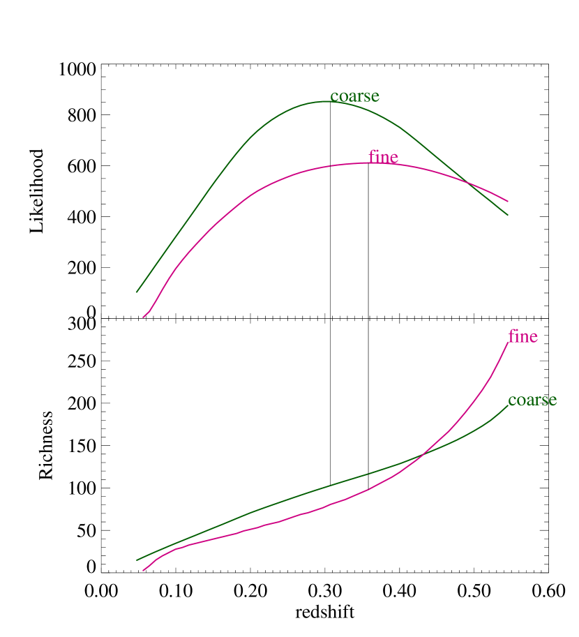
Figure 1: Plots of the “2D” (i.e., $\sigma_{z}\rightarrow\infty$) likelihood and richness as a function of redshift as computed from the coarse and fine matched filters. The input cluster has $z_{c}=0.35$ and a richness ${\Lambda}=100$ (corresponding approximately to Abell richness class 1).

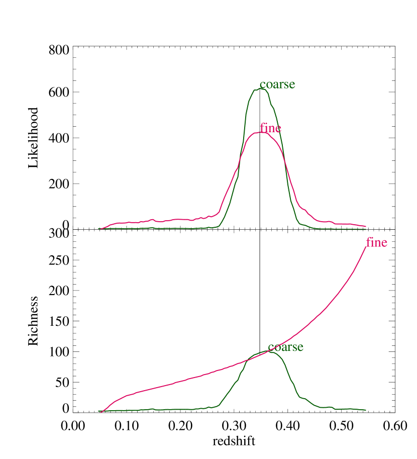
Figure 2: Plots of the “2${\text@frac{1}{2}}$D” ($\sigma_{z}\sim 0.05$) likelihood and richness as a function of redshift as computed from the coarse and fine matched filters. The input cluster has $z_{c}=0.35$ and a richness ${\Lambda}=100$. Although ${\Lambda}_{\rm fine}$ is not peaked like ${\Lambda}_{\rm coarse}$ this difference does not diminish the accuracy since the location of $z_{c}$ is determined entirely by ${\cal L}_{\rm fine}$, which is sharply peaked.

The likelihood functions derived in the previous section represent the core of the AMF cluster detection scheme. Both likelihood functions begin with picking a grid of locations over the survey area for which ${\cal L}$ and ${\Lambda}$ are computed over a range of redshifts. Figures 1 and 2 show the functions ${\cal L}(z)$ and ${\Lambda}(z)$ for a position on the sky located at the center of a ${\Lambda}=100$ cluster ($\sim\frac{2}{3}$ the richness or luminosity of Coma) at $z=0.35$ (the details of the test data are given in the next section). Figure 1 shows the results when no redshift estimate exists (i.e., $\sigma_{z}\rightarrow\infty$), and figure 2 shows what happens when using estimated redshifts with $0.03<\sigma_{z}<0.06$.

Figures 1 and 2 illustrate three of the basic properties of these likelihood functions, which were discussed in the previous section: 1. the dramatic effect of including estimated redshifts on sharpening the peak in ${\cal L}$, which makes finding clusters much easier; 2. the qualitative difference in the form of ${\Lambda}_{\rm fine}(z)$ and ${\Lambda}_{\rm coarse}(z)$ in figure 2 that arises from the fact that ${\Lambda}_{\rm coarse}$ is a simple function of ${\cal L}_{\rm coarse}$ while ${\Lambda}_{\rm fine}$ is a complicated function of ${\cal L}_{\rm fine}$; 3. the shortward bias in the cluster redshift as computed from ${\cal L}_{\rm coarse}$ in 2D (figure 1), which is a general bias in the 2D coarse likelihood function (for a discussion of how to correct for this bias see Postman et al (1996)). In the 3D case, the coarse likelihood of rich clusters has comparable accuracy to the fine likelihood. For poorer clusters (${\Lambda}<50$), the coarse likelihood yields higher richness estimates than the true values; this is a result of the Gaussian assumption used for deriving the coarse likelihood which worsens for poorer clusters.

Implementation of the AMF cluster selection consists of five steps: (1) reading the galaxy catalog, (2) defining and verifying the model, (3) computing ${\cal L}_{\rm coarse}$ over the entire galaxy survey over a range of redshifts, (4) finding clusters by identifying peaks in the ${\cal L}_{\rm coarse}$ map, and (5) evaluating ${\cal L}_{\rm fine}$ and obtaining a more precise determination of each cluster’s redshift and richness.

3.1 Reading the Galaxy Catalog

The first step of the AMF is reading the galaxy catalog over a specified region of the sky. The galaxy catalog consists of four to six quantities for each galaxy, $i$: the position on the sky RA_i and DEC_i, the apparent luminosity (i.e. flux) in specific band $l_{i}$, the Hubble type used for determining the K correction $\mu_{i}$ (e.g., E, Sa or Sc), the estimated redshift $z_{i}$ and estimated error $\sigma_{z}^{i}$. In the case of a single band survey, where no photometric redshifts are possible, $z_{i}$ and $\sigma_{z}^{i}$ will not exist. In addition to these local quantities, the following global quantities are computed from the catalog: the apparent luminosity limit $l_{\rm min}$, the mean estimated error $\bar{\sigma}_{z}$. Finally, it is necessary to set the minimum and maximum cluster redshifts for the cluster search $z_{\rm min}$ and $z_{\rm max}$.

3.2 Model Definition and Verification

The primary model components which need to be specified are: the cluster radial profile $\Sigma_{c}(r)$, the cluster luminosity profile $\phi_{c}(L)$, a normalization convention for the cluster that sets the units of richness ${\Lambda}$, and the field number density versus apparent luminosity distribution $n_{f}(l)$. In addition, a specific cosmological model needs to be chosen along with K corrections for each Hubble type, from which the angular distance $d(z)$ and luminosity distance $D(z,\mu)$ can be computed. The observed galaxy catalog needs to be tested for its consistency with the model parameters (such as $n_{f}(l)$). While this is unnecessary for the simulated galaxy catalog used below (where the model used to find clusters is the same as the one used to generate the catalog), we show some of the consistency checks for illustration purposes (see Appendix D).

3.3 ${\cal L}_{\rm coarse}$ Mapping

Mapping out the coarse likelihood function begins with picking a grid covering the survey area. The most straightforward choice is a uniform grid over the area covered, which is conceptually simple and makes finding peaks in the likelihood easy. However, a uniform grid needs to be exceedingly fine in order to ensure adequate resolution at the highest redshifts, and leads to unacceptable computer memory requirements. Another choice for the grid locations is to use the positions of the galaxies themselves. The galaxy positions are a “naturally” adaptive grid that guarantees sufficient resolution at any redshift while also eliminating unnecessary points in sparse regions. For this reason we choose to use the galaxy positions as the grid locations.

At each grid location (i.e. each galaxy position) ${\cal L}_{\rm coarse}$ is evaluated over a range of redshifts from $z_{\rm min}$ to $z_{\rm max}$. The number of redshift points is set so there is adequate coverage for the given value of $\bar{\sigma}_{z}$. Finding the maximum of the likelihood sets the values of the likelihood, redshift and richness at this point: ${\cal L}_{\rm coarse}^{i}$, $z_{\rm coarse}^{i}$, and ${\Lambda}_{\rm coarse}^{i}$. When this process has been completed for all the galaxies, the result is an irregularly gridded map ${\cal L}_{\rm coarse}^{i}({\rm RA}_{i},{\rm DEC}_{i},z_{\rm coarse}^{i})$. The peaks in this map correspond to the locations of the clusters.

3.4 ${\cal L}_{\rm coarse}$ Cluster Selection

Finding peaks in 3D regularly gridded data is straightforward. Finding the peaks in the irregularly gridded function ${\cal L}_{\rm coarse}^{i}({\rm RA}_{i},{\rm DEC}_{i},z_{\rm coarse}^{i})$ is more difficult. There are several possible approaches. We present a simple method which is sufficient for selecting rich clusters. More sophisticated methods will be necessary in order to find poor clusters that are close to rich clusters.

As a first step we eliminate all low likelihood points ${\cal L}_{\rm coarse}^{i}<{\cal L}_{\rm cut}$, where ${\cal L}_{\rm cut}$ is the nominal detection limit, which is independent of richness or redshift. ${\cal L}_{\rm cut}$ can be estimated from the distribution of the ${\cal L}_{\rm coarse}^{i}$ values (figure 3). The peak in the distribution corresponds to the background while the long tail corresponds to the clusters. Assuming the background is a Gaussian whose mean can be estimated from the location of the peak and whose standard deviation is 0.43 times the Full-Width-Half-Maximum (FWHM), then a given value of ${\cal L}_{\rm cut}$ will lie $N_{\sigma}$ standard deviations from the peak

$$N_{\sigma}\sim\frac{{\cal L}_{\rm cut}-{\cal L}_{\rm peak}}{0.43~{}{\rm FWHM}}~{}.$$ (17)

The values of ${\cal L}_{\rm cut}$ shown in figure 3 were chosen so that $N_{\sigma}\sim 5$, which was sufficiently high that no false detections occurred. To first order, ${\cal L}_{\rm cut}\propto\bar{\sigma}_{z}/\bar{z}$, where $\bar{z}$ is the average depth of the survey and is a function of $l_{\rm min}$.

Step two consists of finding the largest value of ${\cal L}_{\rm coarse}^{i}$, which is by definition the first and most overdense cluster. The third step is to eliminate all points that are within a certain radius and redshift of the cluster. Repeating steps two and three until there are no points left results in a complete cluster identification (above ${\cal L}_{\rm cut}$), with a position, redshift and richness ($\propto$ total luminosity) estimate for each cluster.

3.5 ${\cal L}_{\rm fine}$ Evaluation

The angular position, redshift and richness of the clusters determined by the ${\cal L}_{\rm coarse}$ selection are adequate, but can be complemented by determining the redshift and richness from ${\cal L}_{\rm fine}$. Recall that ${\cal L}_{\rm fine}$ requires 10 to 100 times as many operations to evaluate as compared with ${\cal L}_{\rm coarse}$, and applying it to every single galaxy position can be prohibitive. Evaluating ${\cal L}_{\rm fine}$ on just the clusters found with ${\cal L}_{\rm coarse}$ is trivial and worth doing as it should provide more accurate estimates of the cluster redshift and richness because of the better underlying assumptions that went into its derivation. Thus, the final step in our AMF implementation is to compute $z_{\rm fine}^{i}$ and ${\Lambda}_{\rm fine}^{i}$ using ${\cal L}_{\rm fine}$ on each of the cluster positions obtained with ${\cal L}_{\rm coarse}$.

3.6 Implementation Summary

We summarize the above implementation in the following step-by-step list.

1. Read galaxy catalog

   • Read in RA_i, DEC_i, $l_{i}$, $z_{i}$, $\sigma_{z}^{i}$ and $\mu_{i}$ for each galaxy.

   • Pick $l_{\rm min}$ (survey limit), $z_{\rm min}$ and $z_{\rm max}$ (cluster search limits), and compute average distance error $\bar{\sigma}_{z}$.

2. Model definition

   • Choose $\Sigma_{c}$, $\phi_{c}$, $n_{f}$, $d(z_{c})$ and $D(z,\mu)$.

   • Normalize $\Sigma_{c}$ and $\phi_{c}$.

   • Verify galaxy distributions in $l$ and $z$ with those predicted by model.

3. ${\cal L}_{\rm coarse}$ mapping

   • For each galaxy location (RA_i, DEC_i) choose a range of redshifts within $z_{\rm min}$ and $z_{\rm max}$ with a step size no larger that one half $\bar{\sigma}_{z}$.

   • Compute ${\cal L}_{\rm coarse}$ (eq. 12) and ${\Lambda}_{\rm coarse}$ (eq. 13) for each redshift. Set ${\cal L}_{\rm coarse}^{i}$, ${\Lambda}_{\rm coarse}^{i}$ and $z_{\rm coarse}^{i}$ equal to the values at the maximum of ${\cal L}_{\rm coarse}$.

4. Find peaks in the ${\cal L}_{\rm coarse}$ map

   • Compute ${\cal L}_{\rm cut}$ from the ${\cal L}_{\rm coarse}^{i}$ distribution (e.g. 5-$\sigma$ cut).

   • Find all local maxima in ${\cal L}_{\rm coarse}^{i}({\rm RA}_{i},{\rm DEC}_{i},z_{\rm coarse}^{i})$ where ${\cal L}_{\rm coarse}^{i}>{\cal L}_{\rm cut}$; these are the clusters.

5. Refine cluster redshift and richness estimates with ${\cal L}_{\rm fine}$

   • At the RA and DEC of each cluster found with ${\cal L}_{\rm coarse}$ evaluate ${\cal L}_{\rm fine}$ over the same range of redshifts within $z_{\rm min}$ and $z_{\rm max}$.

   • Compute ${\cal L}_{\rm fine}$ (eq. 14) and ${\Lambda}_{\rm fine}$ (eq. 15) for each redshift. Set ${\cal L}_{\rm fine}^{i}$, ${\Lambda}_{\rm fine}^{i}$ and $z_{\rm fine}^{i}$ equal to the values at the maximum of ${\cal L}_{\rm fine}$. These provide the best estimates for the cluster richness and redshift.

In the next section we describe a simulated galaxy catalog used to test the above AMF implementation.

4 Simulated Test Data

Our test data consists of 72 simulated clusters with different richnesses and redshifts placed in a simulated field of randomly distributed galaxies (for a non-random distribution of field galaxies see section 5). The clusters range from groups to rich clusters with total luminosities from 10 $L^{*}$ to 300 $L^{*}$ (corresponding to Abell richness counts of approximately 7 to 200, or richness classes $\ll$0 to $\sim$4) and are distributed in redshift from 0.1 to 0.5. The luminosity profile is a Schechter function with $\alpha=1.1$. The radial profile is a Plummer law given in Appendix A with $r_{\rm max}=1~{}{\rm h^{-1}Mpc}$ and $r_{\rm core}=0.1~{}r_{\rm max}$. The number and absolute luminosity of the field galaxies were generated from a Schechter function, using the field normalization $\phi^{*}=1.08\times 10^{-2}~{}{\rm h}^{3}{\rm Mpc}^{-3}$ (Loveday et al (1992)).

Three different Hubble types were used, E, Sa and Sc, with K corrections taken from Poggianti (1997). Each galaxy in a cluster was randomly assigned a Hubble type so that 60% were E, 30% were Sa, and 10% were Sc; each galaxy in the field is randomly assigned a Hubble type so that 40% were E, 30% were Sa, and 30% were Sc. Knowing the redshift of each galaxy, its absolute luminosity and Hubble type, we can compute the apparent luminosity. All galaxies with apparent luminosity below $r^{\prime}\approx 23.5$ (the anticipated limit of the SDSS) were eliminated. This limit resulted in a field number density of $\sim$5000 galaxies per square degree.

To facilitate the subsequent analysis and interpretation of the results, the clusters were placed on an 8 by 9 grid. The cluster centers were separated by 0.4 degrees, which results in the test data having dimensions of 3.2 by 3.6 degrees. The distribution of the cluster galaxies in RA and DEC is shown in figure 4, where each column has the same richness while each row of clusters is at the same redshift (see figure 6). From left to right the richnesses are $\Lambda=$ 10, 20, 30, 40, 50, 100, 200, and 300. From bottom to top the redshifts are $z_{c}=$ 0.1, 0.15, 0.2, 0.25, 0.3, 0.35, 0.4, 0.45, and 0.5. In all, the clusters contained some 30,000 galaxies, over half of which lie in the richness 200 and 300 clusters. The randomly generated field contained approximately 50,000 galaxies. The distribution of all the galaxies in RA and DEC is shown in figure 5.

So far, the redshifts for the galaxies are exact. If we assume that redshift errors are Gaussian, then we can easily generate offsets to the true positions if we know the standard deviation of the distribution $\sigma_{z}$. Not all the galaxies will have the same estimated redshift error $\sigma_{z}^{i}$, and, in the case of photometric redshifts, these values can be expected to vary by about a factor of two (Connolly et al (1995); Yee (1998)). We model this effect by first randomly generating the estimated redshift errors from a uniform distribution over a specified range (e.g., $0.03<\sigma_{z}^{i}<0.06$). The offsets from the true redshifts are then randomly generated from Gaussian distributions with standard deviations corresponding to $\sigma_{z}^{i}$ values. The estimated redshifts are computed by adding the offsets to the true redshift. Thus, a dataset with $\bar{\sigma}_{z}\sim 0.05$ refers to $0.03<\sigma_{z}^{i}<0.06$.

5 Results and Discussion

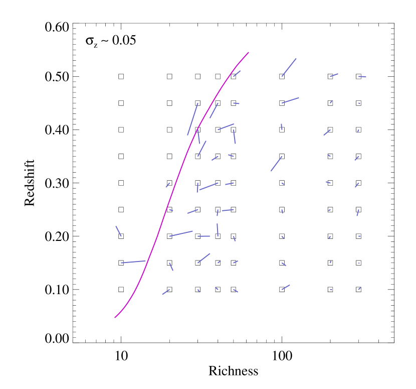
Figure 8: Richness and redshift of each of the input clusters (boxes) with the short lines indicating the corresponding values determined from the AMF fine filter. The long curved line indicates the approximate detection limit and is computed by inserting ${\cal L}_{\rm cut}=40$ into equation (12) and solving for ${\Lambda}$ as a function $z_{c}$.

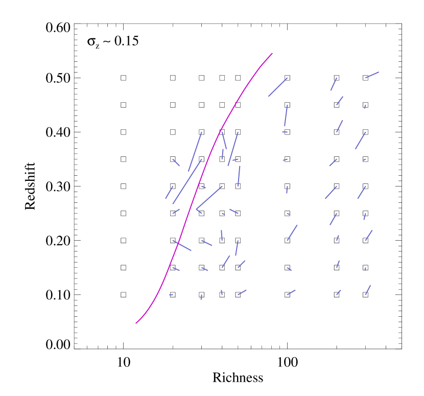
Figure 9: Richness and redshift of each of the input clusters (boxes) with the short lines indicating the corresponding values determined from the AMF fine filter. The long curved line indicates the approximate detection limit and is computed by inserting ${\cal L}_{\rm cut}=100$ into equation (12) and solving for ${\Lambda}$ as a function $z_{c}$.

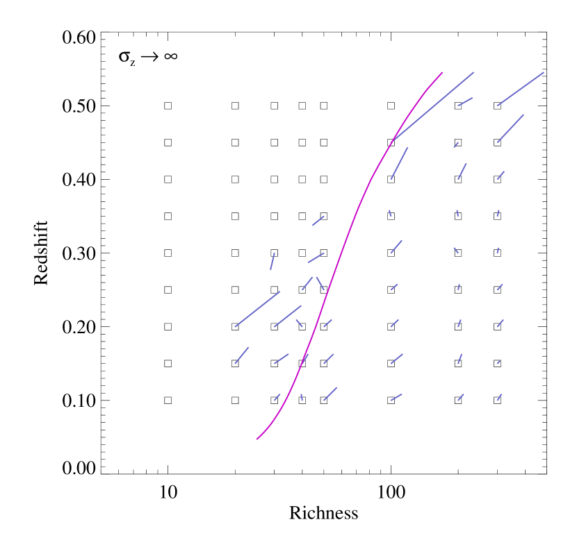
Figure 10: Richness and redshift of each of the input clusters (boxes) with the short lines indicating the corresponding values determined from the fine filter. The long curved line indicates the approximate detection limit and is computed by inserting ${\cal L}_{\rm cut}=300$ into equation (12) and solving for ${\Lambda}$ as a function $z_{c}$.

To test our AMF implementation we ran it on the above simulated galaxy catalog for three different error regimes: $\bar{\sigma}_{z}\sim 0.05$, $\bar{\sigma}_{z}\sim 0.15$ and $\bar{\sigma}_{z}\rightarrow\infty$. A contour plot computed from the maximum likelihood points ${\cal L}_{\rm coarse}^{i}$ is shown in figure 7, which indicates that the coarse filter does a good job of finding the angular positions of the clusters with no false detections. The resulting cluster centers have an accuracy that is within one core radius of the true cluster center. The redshifts and richnesses obtained by applying ${\cal L}_{\rm fine}$ to the clusters found with ${\cal L}_{\rm coarse}$ are shown in figures 8, 9, and 10. The boxes denote the true redshift and richness values of the input clusters. The short lines connect the inputs with the outputs (i.e. the values obtained with ${\cal L}_{\rm fine}$). Smaller lines indicate more accurate redshift and richness determinations. The long curve indicates the expected detection limit for the value of ${\cal L}_{\rm cut}$ used. As expected, the number of clusters detected and their accuracy decrease as $\bar{\sigma}_{z}$ increases. However, nearly all the clusters with ${\Lambda}\gtrsim 100$ (corresponding roughly to Abell richness class $\gtrsim 1$) are detected out to redshifts of 0.5 which is the effective limit of the survey. In a deeper survey it will be possible to detect clusters at higher redshifts.

The errors in the redshift and richness estimates of all detected clusters is presented in figures 11 and 12. A summary of these results is shown in table 1. In general, the AMF finds clusters with an accuracy of $\Delta z\sim 0.02$ in redshift and $\sim$10% in richness. Including distance information lowers the background and results in a substantial improvement in the detection of poorer clusters. Thus, many more clusters are detected when $\sigma_{z}\sim 0.05$ as compared to $\sigma_{z}\rightarrow\infty$. These additional clusters are all poorer and thus have higher errors, which explains why the average errors do not significantly change with $\bar{\sigma}_{z}$.

Table 1: Summary of AMF tests on simulated data

Input	Likelihood	Output	Output
error	cutoff	$z$ error	$\Lambda$ error
$\bar{\sigma}_{z}$	${\cal L}_{\rm cut}$	$\sigma(\Delta z)$	$\sigma(\Delta\Lambda/\Lambda)$
0.05	40	0.014	0.13
0.15	100	0.025	0.12
$\infty$	300	0.023	0.14

Six additional tests were conducted on the $\bar{\sigma}_{z}\sim 0.05$ case to check the robustness of the results. The first test explored the effect of spatial structure in the background distribution of galaxies by using positions taken from an N-body simulation (instead of using randomly distributed field galaxies). The second test investigated the effect of using different K-corrections. The next four tests explored the effect of changing different parameters of the cluster model: $\alpha$ in the Schechter luminosity function, $n$ in the Plummer cluster density profile, the core radius ($r_{\rm core}$) and the maximum radius of the cluster profile ($r_{\rm max}$). The results of all these tests are summarized in Table 2.

The N-body simulation contained $128^{3}$ dark matter particles in a 200 ${\rm h^{-1}Mpc}$ box (Xu (1995)) with sufficient spatial resolution to resolve cluster cores. The final $z=0$ ouput of the simulation was “stacked” in a non-repeating fashion (Gott (1997)) to create a simulated field out to $z=0.6$. Each particle was then assigned a luminosity in the same manner as described earlier for the uniform background. The 72 test clusters were placed in the N-body background. The coarse filter was run on these data using the same parameters as in the uniform case. All the clusters detected with the uniform background were also detected with the N-body background. Next, the fine filter was run on these clusters. There was no change in the estimated redshifts of the clusters. The richness estimates showed a slight increase ($\sim$ 20%) in their variance, which is due to the fluctuations in the background density.

In a real survey, it is unlikely that all the galaxies will have correctly assigned Hubble types. An error in the Hubble type primarily affects the K-correction. To test the effects of incorrect Hubble types we ran the fine filter with an assumption that all the galaxies were Ellipticals (E) and then again assuming that all the galaxies were Spirals (Sc). These changes produced no significant change in the estimated redshift or richness of the clusters out to $z\sim 0.5$.

In the real Universe, clusters can not be described by a single set of model parameters. Two tests of each of four model parameters were carried out to look at the errors produced by using an AMF cluster model with parameters different from the clusters in the data. In each case the fine filter was run on data with $\bar{\sigma}_{z}\sim 0.05$ and the differences in the estimated redshift and richness were examined. The results are summarized in Table 2. None of the changes in any of the parameters significantly affected the estimated redshifts of the clusters. The largest effect on the richness $\Lambda$ occurred with changing the parameter $\alpha$ in the Schechter luminosity function of the cluster. This induced a bias in $\Lambda$ at small redshift; the bias decreases with redshift because the galaxies at high redshift are not part of the faint-end Schechter luminosity function. Changing the slope of the cluster density profile had only a small effect on $\Lambda$. Changing the core radius had no significant effect on $\Lambda$. As expected, $\Lambda$ increases with increasing $r_{\rm max}$.

Table 2: Robustness tests on simulated data with $\sigma_{z}\sim 0.05$. A “no change” entry means that any difference in the estimated redshift or richness was within the nominal errors quoted in Table 1 (i.e., $\Delta z\sim 0.02$ and $\Delta\Lambda/\Lambda\sim 0.1$). Biases are given relative to the nominal value (e.g., a bias of 1.1$\Lambda$ implies that the new estimated richnesss is 1.1 times the nominal estimated richness). All biases are independent of redshift and richness unless stated otherwise.

Model Parameter	New	Effect on	Effect on
(nominal value)	Value	Estimated $z$	Estimated $\Lambda$
Background distribution	N-body	no change	slight ($\sim$ 20%) increase in variance
(uniform)
K correction	all E	no change	no change
(E, Sa and Sc)	all Sc	no change	no change
Cluster lum func slope	-0.8	no change	1.5$\Lambda$ bias at $z\sim 0.1$,
($\alpha=-1.1$)			decreasing to no bias at $z\sim 0.35$
	-1.3	no change	0.5$\Lambda$ bias at $z\sim 0.1$,
			increasing to 1.2$\Lambda$ at $z\sim 0.5$
Cluster profile slope	1.5	no change	1.1$\Lambda$ bias independent of $z$
($n=2.0$)	2.5	no change	0.95$\Lambda$ bias independent of $z$
Cluster core radius	0.05 ${\rm h^{-1}Mpc}$	no change	no change
($r_{\rm core}=0.1~{}{\rm h^{-1}Mpc}$)	0.20 ${\rm h^{-1}Mpc}$	no change	no change
Cluster max radius	0.75 ${\rm h^{-1}Mpc}$	no change	0.75$\Lambda$ bias independent of $z$
($r_{\rm max}=1.0~{}{\rm h^{-1}Mpc}$)	1.25 ${\rm h^{-1}Mpc}$	no change	1.25$\Lambda$ bias independent of $z$

The CPU and memory requirements of the AMF are dominated by the ${\cal L}_{\rm coarse}$ evaluation. The AMF required around 100 MBytes of memory and took from a few minutes ($\bar{\sigma}_{z}\sim 0.05$) to a little under two hours ($\bar{\sigma}_{z}\rightarrow\infty$) using one CPU (198Mhz MIPS R10000) of an SGI Origin200. For example, the SDSS will be composed of approximately 1000 fields similar in size to our test catalog. Since finding clusters in one field is independent of all the others, it is simple to run the AMF on a massively parallel computer; it will be possible to run the AMF on the entire SDSS catalog in one day.

6 Summary and Conclusions

We have presented the Adaptive Matched Filter method for the automatic selection of clusters of galaxies in a wide variety of galaxy catalogs. The AMF can find clusters in most types of galaxy surveys: from two-dimensional (2D) imaging surveys, to multi-band imaging surveys with photometric redshifts of any accuracy (2${\text@frac{1}{2}}$D), to three-dimensional (3D) redshift surveys. The method can also be utilized in the selection of clusters in cosmological N-body simulations. The AMF is based on matching the galaxy catalog with a cluster filter that models the overall galaxy distribution. The model describes the surface density, apparent magnitude, and redshift of cluster and field galaxies. Convolving the data with the filter produces a cluster probability map whose peaks correspond to the location of the clusters. The probability peaks also yield the best fit redshift and richness of each cluster.

The heart of the AMF is the apparent overdensity $\delta_{i}$ which is evaluated at each galaxy position and has a higher value for galaxies in clusters than galaxies in the field. The apparent overdensity distills the entire description of the galaxy catalog into a single function. Two likelihood functions are derived, ${\cal L}_{\rm coarse}$ and ${\cal L}_{\rm fine}$, using different underlying model assumptions. The theoretical framework of the AMF allows estimated redshifts to be included via a simple redshift filter, which effectively limits the sums in ${\cal L}_{\rm coarse}$ and ${\cal L}_{\rm fine}$ to those galaxies within a window around $z_{c}$. The maxima in the likelihood functions are used to identify cluster positions as well as their redshifts and richnesses.

The AMF is adaptive in three ways. First, it adapts to the errors in the estimated redshifts. Second, it uses the locations of the galaxies as “naturally” adaptive grid to ensure sufficient resolution at even the highest redshifts. Third, it uses a two step approach that applies a coarse filter to initially find the clusters and a fine filter to more precisely estimate the redshift and richness of each cluster.

We tested the AMF on a set of simulated clusters with different richnesses and redshifts—ranging from groups to rich clusters at redshifts 0.1 to 0.5; the clusters were placed in a simulated field of randomly distributed galaxies as well as in a non-random distribution produced by N-body cosmological simulations. We find that the AMF detects clusters with an accuracy of $\Delta z\sim$0.02 in redshift and $\sim$10% in richness to $z\lesssim 0.5$ (for a simulated galaxy survey to $r^{\prime}\approx 23.5$). In addition, robustness tests provide a strong indication that the AMF will perform well on observational data sets. Detecting clusters at even higher redshifts will be possible in deeper surveys.

Appendix A Cluster Profile

The projected cluster profile is derived from spherical modified Plummer law profile:

$$\rho_{c}(r)=\left\{\begin{array}[]{c@{\quad,\quad}c}\frac{\rho_{c}^{0}}{(1+r^{2}/r_{\rm core}^{2})^{\frac{n}{2}}}-\frac{\rho_{c}^{0}}{(1+r_{\rm max}^{2}/r_{\rm core}^{2})^{\frac{n}{2}}}&r\leq r_{\rm max}\\ 0&r>r_{\rm max}\end{array}\right.$$ (A1)

where $n\approx 2$ and the constant $\rho_{c}^{0}$ is used to normalize the profile. The projected profile is computed by integrating along the line of sight:

$$\Sigma_{c}(r)=2\int_{r}^{\infty}\frac{\rho_{c}(t)tdt}{\sqrt{t^{2}-r^{2}}},$$ (A2)

which for the modified plummer profile gives

$$\Sigma_{c}(r)=\left\{\begin{array}[]{c@{\quad,\quad}c}\frac{\Sigma_{c}^{0}}{(1+r^{2}/r_{\rm core}^{2})^{\frac{n-1}{2}}}-\frac{\Sigma_{c}^{0}}{(1+r_{\rm max}^{2}/r_{\rm core}^{2})^{\frac{n-1}{2}}}&r\leq r_{\rm max}\\ 0&r>r_{\rm max}\end{array}\right.$$ (A3)

where $\Sigma_{c}^{0}$ is a constants set by the normalization.

Appendix B Luminosity Distance

The transformation between absolute and apparent luminosities in band $\lambda_{0}$

$$L_{\lambda_{0}}=4\pi D^{2}(z;\mu)l_{\lambda_{0}},$$ (B1)

where $\mu$ is the galaxy type (e.g. elliptical, spiral, irregular, …) and $D$ is the luminosity distance at a redshift $z$ and is related to the angular size distance $d$ by

$$D^{2}(z;\mu)=\frac{(1+z)^{2}d^{2}(z)}{K_{\lambda_{0}}(z;\mu)E_{\lambda_{0}}(z;\mu)}~{},$$ (B2)

where $K_{\lambda_{0}}$ and $E_{\lambda_{0}}$ are the“K” and evolutionary corrections. For no evolution models $E_{\lambda_{0}}=1$. The angular-size distance for $\Omega+\Omega_{\Lambda}=1$ cosmologies is given by

$$d(z)=\frac{c}{H_{0}}\int_{0}^{z}\frac{dz^{\prime}}{(1-\Omega+\Omega(1+z^{\prime})^{3})^{1/2}}$$ (B3)

Appendix C Derivation of the Likelihood Functions

Various likelihood functions can be derived. The differences are due to the additional assumptions that are made about the distribution of the observations. This appendix gives the mathematical derivation of the two likelihood functions used in the AMF: ${\cal L}_{\rm coarse}$ and ${\cal L}_{\rm fine}$. Both derivations are conceptually based on virtually binning the data, but make different assumptions about the distribution of galaxies in the virtual bins.

Imagine dividing up the angular and apparent luminosity domain around a cluster into bins. We assign to each bin a unique index $j$. The expected number of galaxies in bin $j$ is denoted $n_{\rm model}^{j}$. The number of galaxies actually found in bin $j$ is $n_{\rm data}^{j}$. In general, the probability of finding $n_{\rm data}^{j}$ galaxies in cell $j$ is given by a Poisson distribution

$$P_{j}=\frac{(n_{\rm model}^{j})^{n_{\rm data}^{j}}e^{-n_{\rm model}^{j}}}{n_{\rm data}^{j}!}$$ (C1)

The likelihood of the data given the model is computed from the sum of the logs of the individual probabilities

$${\cal L}=\sum_{j}\ln P_{j}.$$ (C2)

C.1 Coarse Grained ${\cal L}$

If the virtual bins are made big enough that there are many galaxies in each bin, then the probability distribution can be approximated by a Gaussian

$$P_{j}=\frac{1}{\sqrt{2\pi n_{\rm model}^{j}}}\exp\left\{-\frac{(n_{\rm data}^{j}-n_{\rm model}^{j})^{2}}{2n_{\rm model}^{j}}\right\}~{}.$$ (C3)

Furthermore, if the field contribution is approximately uniform and large enough to dominate the noise then

$$P_{j}=\frac{1}{\sqrt{2\pi n_{f}^{j}}}\exp\left\{-\frac{(n_{\rm data}^{j}-n_{\rm model}^{j})^{2}}{2n_{f}^{j}}\right\}~{}.$$ (C4)

where $n_{\rm model}^{j}=n_{f}^{j}+{\Lambda}n_{c}^{j}$. Summing the logs of these probabilities results in the following expression for the coarse likelihood

$${\cal L}_{\rm coarse} = \sum_{j}\ln P_{j}$$ (C5)

$$= -\frac{1}{2}\sum_{j}\ln 2\pi n_{f}^{j}-\frac{1}{2}\sum_{j}\frac{(n_{\rm data}^{j}-n_{\rm model}^{j})^{2}}{n_{f}^{j}}$$

The first term does not affect the value of ${\Lambda}$ which minimizes ${\cal L}_{\rm coarse}$ and can be dropped. In addition, if the bins can also be made sufficiently small, then the sum over all the bins can be replaced by an integral

$${\cal L}_{\rm coarse}=-\int\frac{(n_{\rm data}(\theta,\l)-n_{\rm model}(\theta,l))^{2}}{n_{f}(\theta,l)}d\Omega dl~{},$$ (C6)

where $n_{\rm data}(\theta,l)$ is a sum of Dirac delta functions corresponding to the locations of the galaxies. Expanding the squared term and replacing $n_{\rm model}$ with $n_{f}+{\Lambda}n_{c}$ yields

$${\cal L}_{\rm coarse}=-\int\frac{n_{\rm data}^{2}-2n_{\rm data}n_{f}-2n_{\rm data}{\Lambda}n_{c}+n_{f}^{2}+2n_{f}{\Lambda}n_{c}+{\Lambda}^{2}n_{c}^{2}}{n_{f}}d\Omega dl~{}.$$ (C7)

The above expression can be simplified by setting $\delta=n_{c}/n_{f}$, dropping all expressions that are independent of ${\Lambda}$, and noting that ${\Lambda}\int n_{c}$ is small compared to the other terms, which leaves

$${\cal L}_{\rm coarse}=2{\Lambda}\sum_{i}\delta_{i}-{\Lambda}^{2}\int\delta(\theta,l)n_{c}(\theta,l)d\Omega dl$$ (C8)

Taking the derivative of ${\cal L}_{\rm coarse}$ with respect to ${\Lambda}$ and setting the result equal to zero, we can solve for $\Lambda_{\rm coarse}$ directly

$$\Lambda_{\rm coarse}=\frac{\sum_{i}\delta_{i}}{\int\delta(\theta,l)n_{c}(\theta,l)d\Omega dl}.$$ (C9)

where the denominator terms of $\phi_{c}$, $\Sigma_{c}$ and $n_{f}$ is

$$\int\delta(\theta,l)n_{c}(\theta,l)d\Omega dl = \int\frac{n_{c}^{2}}{n_{f}}d\Omega dl$$ (C10)

$$= \left[\int^{\infty}_{L(l_{min},z_{c})}\frac{\phi_{c}^{2}(L^{\prime})}{n_{f}(L^{\prime})}dL^{\prime}\right]\left[\frac{d_{c}^{2}}{(1+z_{c})^{2}}\int^{r_{\rm max}}_{0}\Sigma_{c}^{2}(r^{\prime})2\pi r^{\prime}dr^{\prime}\right]~{}.$$

Finally, inserting the above value of $\Lambda_{\rm coarse}$ back into the expression for ${\cal L}_{\rm coarse}$ results in

$${\cal L}_{\rm coarse}={\Lambda}\sum_{i}\delta_{i}~{}~{},$$ (C11)

which is $\Delta_{\rm data}$. Thus, maximizing the measured cluster overdensity will give the correct richness and location of the cluster.

C.2 Fine Grained ${\cal L}$

If the virtual bins are chosen to be sufficiently small that no bin contains more that one galaxy, then the calculation of ${\cal L}$ can be significantly simplified because there are only two probabilities that need to be computed. The probability of the empty bins

$$P_{\rm empty}=e^{-n_{\rm model}^{j}}$$ (C12)

and the probability of the filled bins

$$P_{\rm filled}=n_{\rm model}^{j}e^{-n_{\rm model}^{j}}.$$ (C13)

The sum of the log of the probabilities is then

$${\cal L}_{\rm fine} = \sum_{\rm empty}\ln P_{\rm empty}+\sum_{\rm filled}\ln P_{\rm filled}$$ (C14)

$$= -\sum_{\rm empty}n_{\rm model}^{j}-\sum_{\rm filled}n_{\rm model}^{j}+\sum_{\rm filled}\ln n_{\rm model}^{j}$$

By definition summing over all the empty bins and all the filled bins is the same as summing over all the bins. Thus, the first two terms in equation (C14) are just the total number of galaxies predicted by the model

$$\sum_{\rm all~{}bins}n_{\rm model}^{j} = \int^{\infty}_{l_{\rm min}}\int^{\theta_{\rm max}}_{0}n_{\rm model}(\theta^{\prime},l^{\prime};z_{c})d\Omega^{\prime}dl^{\prime}$$ (C15)

$$= N_{f}+{\Lambda}N_{c}$$

where $l_{min}$ is the apparent luminosity limit of the survey. $N_{f}$ and ${\Lambda}N_{c}$ are the total number of field and cluster galaxies one expects to see inside $\theta_{\rm max}$; they can be computed by integrating $n_{f}$ and $n_{c}$

$$N_{f}(z_{c}) = \pi\theta_{\rm max}^{2}(z_{c})\int^{\infty}_{l_{\rm min}}n_{f}(l^{\prime})dl^{\prime}~{},$$

$$N_{c}(z_{c}) = \int^{\infty}_{l_{\rm min}}\int^{\theta_{\rm max}}_{0}n_{c}(\theta^{\prime},l^{\prime};z_{c})d\Omega^{\prime}dl^{\prime}$$ (C16)

$$= \Phi_{c}(L(l_{\rm min},z_{c}))\int^{r_{\rm max}}_{0}\Sigma_{c}(r^{\prime})2\pi r^{\prime}dr^{\prime}$$

where $\Phi_{c}(L)=\int^{\infty}_{L}\phi_{c}(L^{\prime})dL^{\prime}$.

Because we retain complete freedom to locate the bins wherever we like, we can center all the filled bins on the galaxies, in which case the third term in equation (C14) becomes

$$\sum_{\rm filled}\ln n_{\rm model}^{j}\rightarrow\sum_{i}\ln[n_{f}^{i}+{\Lambda}n_{c}^{i}]~{},$$ (C17)

and the sum is now carried out over all the galaxies instead of all the filled bins. Combining these results we can now write the likelihood in terms that are readily computable from the model and the galaxy catalog

$${\cal L}_{\rm fine}=-N_{f}-{\Lambda}N_{c}+\sum_{i}\ln[n_{f}^{i}+{\Lambda}n_{c}^{i}]~{}.$$ (C18)

The simplest way to find the richness is to take the derivative of the above equation with respect to ${\Lambda}$ and setting it equal to zero yields

$$N_{c}=\sum_{i}\frac{\delta_{i}}{1+\Lambda_{\rm fine}\delta_{i}}~{},$$ (C19)

where we have substituted $\delta_{i}$ for $n_{c}^{i}/n_{f}^{i}$. Unfortunately, it is not possible to solve for $\Lambda_{\rm fine}$ explicitly, but a numerical solution can be found by standard methods. The resulting value of $\Lambda_{\rm fine}$ is then inserted into the following equation for ${\cal L}_{\rm fine}$ to obtain the maximized value of the likelihood

$${\cal L}_{\rm fine}=-\Lambda_{\rm fine}N_{c}+\sum_{i}\ln[1+\Lambda_{\rm fine}\delta_{i}]~{}.$$ (C20)

[Note: in the above expression terms that are independent of $\Lambda_{\rm fine}$ and do not contribute any additional information to ${\cal L}_{\rm fine}$ have been dropped.]

Finally, it is worth mentioning again that while ${\Lambda}_{\rm coarse}$ can be obtained directly from ${\cal L}_{\rm coarse}$, ${\Lambda}_{\rm fine}$ can only be found by numerically finding the zero point of equation (C19). Furthermore, equation (C19) does not lend itself to standard derivative based solvers (e.g., Newton-Raphson) that produce accurate solutions in only a few iterations. Fortunately, the solution can usually be bracketed in the range $0<{\Lambda}_{\rm fine}<1000$, thus obtaining a solution with an accuracy $\Delta{\Lambda}\sim 1$ takes $\log_{2}(1000/1)=10$ iterations using a bisection method.

Appendix D Data/Model Consistency Checks

The first consistency check can be made with $n_{f}(l)$, or its cumulative probability $N_{f}(l)=\int_{l}^{\infty}n_{f}(l^{\prime})dl^{\prime}$, which can be fit directly to the galaxy catalog. In the case where a simulated catalog is used the luminosity distribution is taken from the underlying field luminosity function $\phi_{f}(L)$ and it is possible to compute $N_{f}(l)$ for each Hubble type directly

$$N_{f}(l)=\int_{0}^{\infty}\Phi_{f}(L(l,z,\mu))d(z)^{2}\frac{d(z)}{dz}dz~{},$$ (D1)

where $\Phi_{f}(l)=\int_{l}^{\infty}\phi_{f}(l^{\prime})dl^{\prime}$.

The second consistency check can be made with the distribution in redshift (if estimated redshifts exist), where the number of galaxies at each redshift should satisfy the following convolution with the mean estimated error

$$\frac{dN_{f}}{dz}(z)=\int_{-\infty}^{\infty}\frac{1}{\sqrt{2\pi}\bar{\sigma}_{z}}\exp\left\{-\frac{(z-z^{\prime})^{2}}{2\bar{\sigma}_{z}^{2}}\right\}\Phi_{f}(L(l_{\rm min},z^{\prime},\mu))\frac{d(z^{\prime})}{dz}dz^{\prime}~{}.$$ (D2)

Figure 3: Distribution of ${\cal L}_{\rm coarse}$ values. The range has been chosen so the distributions appear similar. The left dashed line denotes the value of the peak of the distribution. The right dashed line shows the value of ${\cal L}_{\rm cut}$ that was used. The horizontal solid line shows the FWHM around the peak. The significance levels of ${\cal L}_{\rm cut}$ from top to bottom are approximately 8-$\sigma$, 5-$\sigma$ and 5-$\sigma$.

Figure 4: Angular positions of all the simulated cluster galaxies with no background galaxies.

Figure 5: Angular positions of all the simulated cluster and field galaxies.

Figure 6: Richness and redshift of each of the simulated clusters. In this view the cluster parameters match the same 8 by 9 grid used in Figure 4.

Figure 7: Contour plot of ${\cal L}_{\rm coarse}$ computed from simulated data with photometric redshift errors $\sigma_{z}\sim 0.05$. Contour levels begin at ${\cal L}_{\rm coarse}=40$ and increase by a factor of 3 with each subsequent level.

Figure 11: Redshift error as a function of redshift for all the detected clusters. Dashed lines indicate the 1-$\sigma$ error range computed from these data, which from top to bottom are 0.014, 0.025 and 0.023.

Figure 12: Fractional richness error as a function of redshift for all the detected clusters. Dashed lines indicate the 1-$\sigma$ range error computed from these data, which from top to bottom are 0.13, 0.12 and 0.14.

References

- Abell (1958) Abell, G. 1958, ApJS, 3, 211
- Abell, Corwin & Olowin (1989) Abell, G., Corwin, H. & Olowin, R. 1989, ApJS, 70, 1
- Bahcall (1988) Bahcall, N. 1988, ARA&A, 26, 631
- Bahcall & Cen (1992) Bahcall, N. & Cen, R. 1992, ApJ, 398, L81
- Bahcall & Cen (1993) Bahcall, N. & Cen, R. 1993, ApJ, 408, L77
- Bahcall, Fan & Cen (1997) Bahcall, N., Fan, X. & Cen, R. 1997, ApJ, 485, L53
- Bahcall, Lubin & Dorman (1995) Bahcall, N., Lubin, L. & Dorman, V. 1995, ApJ, 447, L81
- Bertschinger & Gelb (1991) Bertschinger, E. & Gelb, J. 1991, Computers in Physics, 5, 164
- Binggeli, Sandage & Tammann (1988) Binggeli, B., Sandage, A. & Tammann, G. 1988 ARA&A, 26, 509
- Carlberg et al (1996) Carlberg, R., Yee, H., Ellingson, E., Abraham, R., Gravel, P., Morris, S. & Pricthet, C. 1996 ApJ, 462, 32
- Carlberg et al (1997) Carlberg, R., Morris, S., Yee, H. & Ellingson, E. 1997 ApJ, 478, L19
- Connolly et al (1995) Connolly, A., Szalay, A., Bershady, M., Kinney, A. & Calzetti, D. 1995, AJ, 110, 2655
- Dalton, Maddox & Sutherland (1997) Dalton, G., Maddox, S. & Sutherland, W. 1997, MNRAS, 289, 263
- Dalton et al (1994) Dalton, G., Efstathiou, G., Maddox, S. & Sutherland, W. 1994, MNRAS, 269, 15
- Efstathiou et al (1988) Efstathiou, G., Frenk, C.S., White, S.D.M. & Davis, M. 1988, MNRAS, 235, 715
- Eke, Cole & Frenk (1996) Eke, V., Cole, S. & Frenk, C. 1996, MNRAS, 282, 263
- Evrard (1989) Evrard, A. 1989, ApJ, 341, L71
- Gelb & Bertschinger (1994) Gelb, J. & Bertschinger, J. 1994, ApJ, 436, 467
- Gott (1997) Gott, J.R. 1997, personal communication
- Henry et al (1992) Henry, J. et al 1992, ApJ, 386, 408
- Huchra et al (1990) Huchra, J. Geller, M., Henry, P. & Postman, M. 1990, ApJ, 365, 66
- Kawasaki et al (1997) Kawaski, W., Shimasaku, K., Doi, M. & Okamura, S. 1997 astro-ph/9705112, accepted A&AS
- Kaiser & Squires (1993) Kaiser, N. & Squires, G. 1993, ApJ, 404, 441
- Kleyna et al (1996) Kleyna, J.T., Geller, M.J., Kenyon, S.J. & Kurtz, M.J. 1996, AJ, 113, 624
- Loveday et al (1992) Loveday, J., Peterson, B., Efstathiou, G. & Maddox, S. 1992 ApJ, 390, 338
- Lubin & Postman (1996) Lubin, L., & Postman, M. 1996, AJ, 111, 1795
- Lubin (1996) Lubin, L., & Postman, M. 1996, AJ, 112, 23
- Lumsden et al (1992) Lumsden, S., Nichol, R., Collins, C. & Guzzo, L. 1992, MNRAS, 258, 1
- McGill & Couchman (1990) McGill, C. & Couchman, H. 1990, ApJ, 364, 426
- Oukbir & Blanchard (1997) Oukbir, J. & Blanchard, A. 1997, A&A, 317, 1
- Peacock & Dodds (1994) Peacock, P.J.E. & Dodds, S. 1994 MNRAS, 267, 1020
- Peebles, Daly & Juszkiewicz (1989) Peebles, P.J.E., Daly, R. & Juszkiewicz, R. 1989 ApJ, 347, 563
- Peebles (1993) Peebles, P.J.E. 1993 Principles of Physical Cosmology
- Poggianti (1997) Poggianti, B. 1997 A&AS, 122, 399
- Postman, Huchra & Geller (1992) Postman, M., Huchra, J. & Geller, M. 1992, ApJ, 384, 404
- Postman et al (1996) Postman, M. et al 1996, AJ, 111, 615
- Schechter (1976) Schechter, P. 1976, ApJ, 203, 297
- Schuecker & Bohringer (1998) Schuecker, P. & Bohringer, H. 1998, astro-ph/9809396, to appear in A&A
- Suto, Cen & Ostriker (1992) Suto, Y., Cen, R. & Ostriker, J.P. 1992, ApJ, 395, 1
- Tyson, Valdes & Wenk (1990) Tyson, J.A., Valdes, F. & Wenk, R.A. 1990, ApJ, 349, L1
- Xu (1995) Xu, G., 1995, Ph.D. Thesis, Princeton University
- Yee (1998) Yee, H.K. to appear in the proceedings of the Xth Recontres de Blois: Birth of Galaxies, Blois, France, July 1998
- Zwicky (1957) Zwicky, F. 1957, Morphological Astronomy, Springer-Verlag
- Zwicky et al 1961- (68) Zwicky, F., Herzog, E., Wild, P., Karpowicz, M. & Kowal, C. 1961-68, Catalog of Galaxies and Clusters of Galxies, Vol. 1-6, CalTech