A CATALOG OF 200 GALAXY CLUSTERS SERENDIPITOUSLY DETECTED IN THE ROSAT PSPC POINTED OBSERVATIONS

Abstract

We present a catalog of 200 clusters of galaxies serendipitously detected in 647 ROSAT PSPC high Galactic latitude pointings covering 158 square degrees. This is one of the largest X-ray selected cluster samples, comparable in size only to the ROSAT All-Sky Survey sample of nearby clusters (Ebeling et al. 1997). We detect clusters in the inner 17.5′ of the ROSAT PSPC field of view using the spatial extent of their X-ray emission. Fluxes of detected clusters range from $1.6\times 10^{-14}$ to $8\times 10^{-12}\,$ergs s${}^{-1}\,$cm^-2 in the 0.5–2 keV energy band. X-ray luminosities range from $10^{42}~{}$erg s^-1, corresponding to very poor groups, to $\sim 5\times 10^{44}\,$erg s^-1, corresponding to rich clusters. The cluster redshifts range from $z=0.015$ to $z>0.5$. The catalog lists X-ray fluxes, core-radii, spectroscopic redshifts for 73 clusters and photometric redshifts for the remainder. Our detection method, optimized for finding extended sources in the presence of source confusion, is described in detail. Selection effects necessary for a statistical analysis of the cluster sample are comprehensively studied by Monte-Carlo simulations.

We have optically confirmed 200 of 223 X-ray sources as clusters of galaxies. Of the remaining 23 sources, 18 are likely false detections arising from blends of unresolved point X-ray sources, and for 5 we have not obtained deep CCD images. Above a flux of $2\times 10^{-13}\,$ergs s${}^{-1}\,$cm^-2, 98% of extended X-ray sources are optically confirmed clusters. The $\log N-\log S$ relation for clusters derived from our catalog shows excellent agreement with counts of bright clusters derived from the Einstein Extended Medium Sensitivity Survey (Henry et al. 1992) and ROSAT All-Sky Survey (Ebeling et al. 1997). At fainter fluxes, our $\log N-\log S$ relation agrees with the smaller-area WARPS survey (Jones et al. 1998). Our cluster counts appear to be systematically higher than those from a 50 deg² survey of Rosati et al. (1998). In particular, at a flux of $2\times 10^{-13}\,$ergs s${}^{-1}\,$cm^-2, we find a surface density of clusters of $0.57\pm 0.07$ per square degree, which is a factor of 1.3 more than found by Rosati et al. This difference is marginally significant at the $\sim 2$ sigma level. The large area of our survey makes it possible to study the evolution of the X-ray luminosity function in the high luminosity range inaccessible with other, smaller area ROSAT surveys.

1. Introduction

Clusters of galaxies are among the most important objects for cosmological studies. Models of large scale structure formation such as CDM, predict that the abundance of clusters is determined by the spectrum of primordial perturbations and cosmological parameters $\Omega$ and $\Lambda$. Observations of clusters at different redshifts can be used to constrain these parameters (e.g., White & Rees 1978, Kaiser 1986, White, Efstathiou, & Frenk 1993, Henry & Arnaud 1991, Viana & Liddle 1996, Henry 1997). Following a different approach, observations of the Sunyaev-Zel’dovich effect (Sunyaev & Zel’dovich 1972) in a large sample of distant clusters can be used for a direct measurement of the distance to these clusters, and thus provide the values of $H_{0}$ (e.g., Birkinshaw, Hughes, & Arnaud 1991) and $q_{0}$.

Up until the present, the largest samples of distant clusters resulted from optical surveys that searched for enhancements in the surface density of galaxies (e.g., Postman et al. 1996). This method suffers seriously from projection effects (e.g., van Haarlem et al. 1997). Distant clusters found by such techniques as galaxy concentrations around distant radio sources (Dickinson 1996) or “dark” lenses (Hattori et al. 1997) cannot be considered as statistical samples. Of all methods for detecting distant clusters, X-ray surveys are the least sensitive to projection, because the X-ray emission is proportional to the square of the density of the hot gas, which must be compressed in a deep potential well for us to detect it. It is noteworthy that unlike optical, X-ray surveys have the possibility of finding interesting objects such as “fossil” clusters in which almost all galaxies have merged to form a cD galaxy (Ponman et al. 1994), and hypothetical “failed” clusters in which galaxy formation was suppressed (Tucker et al. 1995). To date, the largest published sample of distant X-ray selected clusters is that from the Einstein Extended Medium Sensitivity Survey (EMSS; Goia et al. 1990, Stocke et al. 1991). However, because of the relatively high flux limit, the EMSS sample contains only 6 clusters at $z>0.5$.

Finding clusters in X-rays is complicated by their rarity among other types of sources. A comparison of the $\log N-\log S$ relations for all sources (Hasinger et al. 1993a) and clusters (this work) shows that at a flux of $10^{-14}\,$ergs s${}^{-1}\,$cm^-2 in the 0.5–2 keV band, clusters comprise not more than 10–20% of the total source population. The large amount of optical identification work needed for cluster selection can be greatly reduced if they are searched for among spatially extended X-ray sources. Even at $z=1$, a rich cluster with a core-radius of 250 kpc has an angular radius of $>20\arcsec$, which still can be resolved with the ROSAT PSPC on-axis. Detection of extended sources requires new analysis techniques. Even if the spatial extent is not used for cluster selection, special detection techniques are needed because clusters at $z\approx 0.2-0.3$ are 3–4 times broader than the ROSAT PSPC point spread function.

The idea of selecting distant cluster samples from various ROSAT surveys was pursued by different groups in the past few years. Rosati et al. (1995, 1998) searched for clusters in long exposure ($>15$ ksec) ROSAT PSPC pointed observations with a total area of 50 deg², using optical identifications of all extended X-ray sources found by wavelet transform analysis. Their sample consists at present of 70 clusters. The Wide Angle ROSAT Pointed Survey (WARPS, Scharf et al. 1997, Jones et al. 1998) uses the Voronoi Tessellation and Percolation technique to detect both point-like and extended sources, followed by optical identifications of all sources. The WARPS cluster sample consists at present of 46 clusters found in ROSAT pointings with exposures $>8$ ksec, covering 16.2 deg². A small sample of 15 clusters at $0.3<z<0.7$ was identified by the SHARC survey (Collins et al. 1997). The RIXOS cluster sample (Castander et al. 1995) consists of 13 clusters, detected using a technique which was optimized for point sources. Their results on cluster evolution appear to contradict other ROSAT surveys (Collins et al. 1997), probably because the point source detection algorithm had a low efficiency for detecting extended cluster emission. Finally, important information about the surface density of clusters at very low fluxes is provided by several very deep ROSAT pointings in which complete optical identifications are performed (e.g. McHardy et el. 1997). Note that because of the small area, none of the aforementioned surveys is able to study the luminosity function of distant clusters above $3\times 10^{44}$ ergs s^-1, where the deficit of high redshift EMSS clusters was reported (Henry et al. 1992).

In this paper, we present a sample of distant clusters selected from 647 ROSAT PSPC observations of high Galactic latitude targets, covering a solid angle of 158 square degrees, a factor of three larger than the largest of the other ROSAT surveys. The source catalog includes 200 optically confirmed clusters, and thus is one of the largest X-ray selected samples, comparable in size only to the ROSAT All-Sky Survey sample of nearby clusters (Ebeling et al. 1997). We detect cluster candidates as extended X-ray sources using the wavelet decomposition technique described in this paper and Maximum Likelihood fitting of the surface brightness distributions to determine the significance of the source extent. We then identify only significantly extended sources with optical follow-up observations. Optical observations confirm that 90% of our sources are indeed clusters of galaxies. Various selection effects such as the fraction of clusters which remain unresolved or undetected, are studied using extensive Monte-Carlo simulations. Comparison of the $\log N-\log S$ relation for clusters derived from our and other ROSAT surveys shows that our cluster counts at the bright end are in excellent agreement with those from the ROSAT All-Sky Survey sample of Ebeling et al. (1997). At a flux of $2\times 10^{-13}\,$ergs s${}^{-1}\,$cm^-2, our $\log N-\log S$ relation agrees well with the WARPS survey (Jones et al. 1998), but is somewhat higher than that found by Rosati et al. (1998).

Cluster size and flux estimates throughout the paper use $H_{0}=50$ km s^-1 Mpc^-1 and $q_{0}=0.5$. All X-ray fluxes and luminosities are reported in the 0.5–2 keV energy band.

2. X-ray data

We analyzed only ROSAT PSPC pointings at high Galactic latitudes, $|b|>30^{\circ}$, and low absorption, $N_{H}<6\times 10^{20}\,$cm^-2, excluding the 10^∘ radius regions around the LMC and SMC. Low Galactic latitude fields were not used because the absorption is large and nonuniform in these regions, and because a high density of stars complicates optical identifications. We also excluded observations of extended targets, such as known clusters of galaxies, nearby galaxies, SNRs, and star clusters. As the only exception, we included the 2146+0413 pointing (ROSAT sequences 800150 and 800150a01) which was an X-ray follow-up of clusters selected optically in a blank field.

All individual ROSAT sequences with listed exposures longer than 2 ksec, meeting the above criteria and publicly available by April 1996, were extracted from the data archive at GSFC. Using S. Snowden’s software, we cleaned the data excluding high background intervals. We also generated exposure maps using R4–R7 detector maps (energy range 0.5–2 keV) weighted according to the average PSPC background spectrum. Multiple observations of the same target were merged. Observations with cleaned exposures $<1.5$ ksec were discarded. The final dataset consists of 647 fields, schematically shown in Galactic coordinates in Fig 2. We used only hard band images, 0.6–2 keV, which increases the sensitivity of cluster detection given that the spectrum of the ROSAT background is much softer than that of a typical cluster. This energy band is slightly different from that used for the exposure map generation, but this discrepancy results only in a very small, $<2\%$, error in the vignetting correction in the inner region of the field of view where clusters are detected. To oversample the PSF adequately, an image pixel size of 5″ was chosen.

The distribution of ROSAT pointings in Galactic coordinates. The higher density in the Northern hemisphere is caused by a preferential choice of Northern objects as ROSAT targets.

Our next step was to calculate the background map for each observation. The ROSAT PSPC background cannot be modeled simply using the exposure map template because of the non-uniformity of the cosmic X-ray background, the presence of scattered solar X-rays, and the wings of the PSF around bright sources. The angular correlation function of the XRB (Vikhlinin & Forman 1995, Soltan et al. 1996) predicts $\approx 10\%$ brightness fluctuations on a $10\arcmin$ scale. If not modeled, such background variations can cause errors in measured cluster fluxes. Since the best approximation to the background in each field is a smoothed source-subtracted image, we created background maps as follows. We first divided an image by its exposure map to remove the imprint of the PSPC window support structure. Using the wavelet decomposition technique (§3.2), we subtracted all sources with characteristic sizes $\leq 3\arcmin$ in radius and smoothed the cleaned image with a $\sigma=6\arcmin$ Gaussian. The background map was finally obtained as a product of the smoothed image and the exposure map.

3. Detection of extended sources

3.1. General Considerations

Finding clusters in ROSAT PSPC images requires detection of sources of widely different angular size ranging from approximately the FWHM of the PSF, $\sim 25\arcsec$, to several arcminutes. Any algorithm for finding spatially extended sources solves two tasks: A) source detection, i.e. identifying regions where the surface brightness significantly exceeds that of the background, and B) determining extent, i.e. deciding whether the detected source is significantly broader than the point spread function. The two-stage nature of extended source detection is not usually emphasized, but can be seen in practice. Rosati et al. (1995) convolved images with wavelet kernels of varying scale to find sources and then derived the source extent from wavelet amplitudes. Scharf et al. (1997) used Voronoi Tessellation and Percolation (VTP) to find regions with enhanced surface brightness and then derived the source extent from the measured area and flux. Each of these methods has advantages for certain tasks. For example, VTP can find extended sources regardless of their shape. However, none of these methods is optimal for both parts of the problem. Obviously, the best sensitivity can be achieved if, at each stage, one uses a separate algorithm optimized for its task. We show below that our method of detecting sources using wavelets and determining source extent by Maximum Likelihood fitting is theoretically close to optimum for finding regularly-shaped clusters.

The optimal method of source detection is matched filtering (e.g. Pratt 1978). For faint sources, the filter is close in shape to the sources themselves, and any filter with a shape close to the matched one performs almost equally well (Press et al. 1992). Our wavelet detection method uses filters which approximate Gaussians with $\sigma=1,2,4,\ldots$ pixels. Since these filters span a range of sizes, nearly optimal detection is achieved for circular sources of any size. With an axially-symmetric filter, it is possible to miss very irregular sources. However, most clusters are relatively regular (Jones & Forman 1998) for detection purposes. Also, this shortcoming is clearly outweighed by the merits of the wavelet method, such as optimal detection of sources with regular shape, complete background subtraction and elimination of the influence of point sources. We discuss these issues below in detail.

Consider now the optimal method to discriminate between extended and point sources. Cluster radial surface brightness profiles can be described by the so called $\beta$-model, $I(r,r_{c})=I_{0}\,(1+r^{2}/r_{c}^{2})^{-3\beta+0.5}$ (e.g. Cavaliere & Fusco-Femiano 1976). Therefore, to discriminate between a cluster and a point source, we should determine whether $I(r,r_{c})$ with core radius $r_{c}>0$ describes the data better than a $\delta$-function, that is, $I(r,r_{c})$ with $r_{c}=0$. According to the Neyman-Pearson Lemma (e.g. Martin 1971), the most sensitive test for this problem is the change in the value of the likelihood function between the best-fit value of $r_{c}$ and $r_{c}=0$. Maximum Likelihood fitting may not be the best method for finding clusters with arbitrary shape, but theoretically it is the best one for the vast majority of clusters having regular shape.

Based on the considerations above, we implemented an algorithm for detection of extended sources which uses our own variant of wavelet transform analysis, wavelet decomposition, to find all sources even in the presence of source confusion and Maximum Likelihood fitting of $\beta$-models to determine whether each source is extended. Each step is discussed below in detail.

3.2. Wavelet Detection of Cluster Candidates

Cluster detection in the ROSAT PSPC images is complicated by the varying background and confusion with point sources located in the vicinity of clusters. The wavelet transform is well-suited to overcome these difficulties. We briefly outline the relevant properties of the wavelet transform and then describe our particular implementation.

3.2.1 General Properties of the Wavelet Transform

The basic idea of the wavelet transform applied to astronomical images (e.g. Grebenev et al. 1995 and references therein) is a convolution with a kernel which consists of a positive core and an outer negative ring, so that the integral of the kernel over the $x,y$ plane is zero. The convolution with such kernels allows complete background subtraction and isolation of structures of particular angular size. This can be shown using a kernel which is the difference of two Gaussians:

$$W(r)\;=\;\frac{\exp(-r^{2}/2a^{2})}{2\pi a^{2}}\;-\;\frac{\exp(-r^{2}/2b^{2})}{2\pi b^{2}},$$ (1)

where $b=2a$. The convolution of this kernel with any linear function $s(x,y)=ax+by+c$ is zero. Therefore, any slowly varying background which can be locally approximated by a linear function is subtracted by a convolution with this kernel. To demonstrate the ability of wavelets to reveal structures with a given size, consider the convolution of the wavelet kernel with a Gaussian $\exp(-r^{2}/2\sigma^{2})$. The convolution amplitude achieves its maximum when $\sigma=a\sqrt{2}$ but rapidly falls to $1/2$ of the maximum for $\sigma=a/2$ and $\sigma=4a$. These properties of the wavelet transform are used for source detection (e.g., Damiani et al. 1997). In most applications, an image is convolved with a family of kernels of the same functional form while varying its scale ($a$ in eq. 1). Sources are detected as significant local maxima in the convolved images. Information about the source angular extent can be derived from the wavelet transform values at different scales. This simple approach works well for detection of isolated sources, but fails if another bright source is located nearby, as is shown in Fig. 1a,b. A point source with a flux four times that of the cluster is located at $2/3$ core-radii from the cluster center (a). The image is convolved with the wavelet kernels (eq.1) of scale $a=1,2,4,\ldots,32$ pixels (b). At each scale, the point source dominates the convolution, and the cluster remains undetected. A different kind of complication for a simple wavelet analysis is caused by compact groups of point sources. Convolved with a wide kernel, such groups appear as a single extended source, resulting in false cluster detections. Neither of these problems can be overcome by using a different symmetric wavelet kernel with compact support (Strag & Nguyen 1995). However, they can be overcome using the idea employed in the CLEAN algorithm commonly applied in radio astronomy (Högbom 1974): point sources are detected first and subtracted from the image before the detection of extended sources. Below we describe our algorithm, which we call wavelet decomposition, which combines this approach with wavelet transform analysis.

3.2.2 Wavelet Decomposition

The family of wavelet kernels we use is given by eq. 1, in which we use several combinations of $a$ and $b$ which we call scales. At scale 1, the positive component in eq.1 is a $\delta$-function ($a=0$) and $b=1$ pixel. At scale 2, $a=1$ and $b=2$ pixels, at scale 3, $a=2$ and $b=4$ pixels and so on. At the largest scale $n$, the kernel is a single, positive Gaussian with $a=2^{n-1}$ pixels. How close is this family of kernels to the optimal filter for detecting sources with the $\beta$-model surface brightness profiles? Numerical calculations show that in at least one of the scales, the signal-to-noise ratio exceeds 80% of the maximum value corresponding to the optimal filter — the $\beta$-model itself — for $0.55<\beta<0.8$.

The described family of wavelet kernels has the advantage of an easy and linear back-transformation. The original image $z(x,y)$ is given by

$$z(x,y)=\sum_{j=1}^{n}w_{j}(x,y),$$ (2)

where $w_{j}(x,y)$ is the convolution with the kernel of scale $j$. An important interpretation of this wavelet transform follows from this equation: it provides a decomposition of an image into a sum of components of different characteristic sizes. With this interpretation, we construct the following iterative scheme to remove the effect of point sources.

We convolved the image with a kernel of the smallest scale, estimated the detection threshold as described below, and cleaned the image of noise. The convolved image values were preserved in those regions where the brightness exceeded $1/2$ of the detection threshold and which contained at least one maximum above the detection threshold. The remaining image was set to zero. We subtracted this cleaned image from the input image to remove the sources that have been detected at this step, and repeated the convolution and cleaning procedure iteratively until no more sources were detected at this scale. We also added cleaned images obtained at each iteration to produce a composite image of significant sources detected at this scale. We then moved to the next scale, at which the input image was set to the original image minus everything detected at the first scale. The iterations were stoped at scale 6, for which $a=80\arcsec$ and $b=160\arcsec$ and detected sources have typical full widths of 3′–4′.

The bottom panels of Fig. 1 illustrate this procedure. The smallest wavelet kernel is insensitive to the broad cluster emission and detects only the point source. When iterations at scale 1 are completed, $\sim 90\%$ of the point source flux has been subtracted. Subtraction of the point source continues at scales 2 and 3, while the cluster remains undetected because it is broader than the analyzing kernel. The point source is almost completely subtracted at small scales and does not interfere with cluster detection at scales 4–6. The result of these iterations is a set of images containing statistically significant structures detected at each scale, whose characteristic size corresponds to the width of the analyzing kernel at this scale. Therefore, to separate point and extended sources, one can combine small and large scales, respectively. As Fig. 1d shows, the sum of scales 1–3 and 4–6 provides almost perfect separation of the original image into the point source and the cluster.

It is important to choose the correct detection thresholds. Although several analytic methods of deriving detection thresholds for the wavelet transform were suggested (Starck & Pierre 1998 and references therein), we determined them through Monte-Carlo simulations. We simulated $512\times 512$ images consisting of a flat Poisson background and convolved them with the wavelet kernels. The distribution of the local maxima in the convolved images was used to define the detection threshold. We set this threshold at that value above which one expects to find on average $1/3$ local maximum per simulated background image per scale in the absence of real sources, so that in the combined scales 4–6 we expect one false detection per image. Thus defined, detection thresholds correspond to a formal significance of $\approx 4.5\sigma$. Detection thresholds were tabulated for a grid of simulated background intensities. In the analysis of real images, we estimated the local background and found the detection threshold by interpolation over the precalculated grid. Detection thresholds were deliberately set low, allowing approximately 600 false detections in the entire survey, since our goal at this step was to detect all possible candidates for the subsequent Maximum Likelihood fitting, where the final decision about source significance and extent is made.

Figure 1.— Advantage of the wavelet decomposition algorithm. A bright point source is located in the vicinity of a cluster (a). Dashed lines show the strip in which brightness profiles (panels b–d) were extracted. Panel (b) shows the result of convolution of this image with wavelet kernels (eq.1) with the scale $a=1,2,4,\ldots,32$ pixels. The data profile is shown by the solid histogram, and the profiles of convolved images by solid lines. At all scales, the convolution is dominated by the point source and there is no separate peak corresponding to the cluster. Therefore, the cluster remains undetected by this simple analysis. Our method (c) provides a decomposition of the original image into components with the characteristic size 1, 2, 4, $\ldots$, 32 pixels. Small-scale components model the point source. The cluster becomes apparent and well-separated from the point source at large scales. The sum of the three smallest and three largest scales of the wavelet decomposition provide almost perfect decomposition of the raw image into its original components (d).

As a result of the wavelet decomposition, we obtain six images which contain detected sources of characteristic size (FWHM) approximately $7\arcsec,15\arcsec,30\arcsec,60\arcsec,120\arcsec,240\arcsec$ (scales 1 through 6). We use these images to select candidate extended sources for subsequent modeling. Since the FWHM of the PSF is 25″ on-axis, most point sources are detected on scales 1–3 and are absent at scales 4–6. On the other hand, a distant cluster with core radius of 250 kpc at $z=0.5$ has an angular radius of 35″ (equivalent to $\sim 70\arcsec$ FWHM) and hence is detected at scales 4–6, to which point sources do not contribute. Even clusters with smaller core radii, $\sim 10\arcsec$, would be detected at scale 4, because their surface brightness profiles become broader than $\sim 30\arcsec$ FWHM when blurred by the PSF. Therefore, cluster candidates can be selected as sources detected at scale 4 or higher. Some point sources, especially those at large off-axis angles where the angular resolution degrades, are detected at scale 4. This shows that our cluster candidate selection based on the wavelet decomposition is lenient, and we are unlikely to miss any real clusters at this step. The next step is the Maximum Likelihood fitting of selected candidate extended sources to determine the significance of their extent and existence, which will be used for the final cluster selection.

3.3. Maximum Likelihood Fitting of Sources

3.3.1 Isolated Clusters

The procedure is straightforward for isolated extended sources. The photon image is fit by a model which consists of the $\beta$-model convolved with the PSF. Source position, core-radius, and total flux are free parameters, while $\beta$ is fixed at a value of $2/3$. The model also includes the fixed background taken from the map calculated as described in §2. The PSF is calculated at the appropriate off-axis angle for a typical source spectrum in the 0.6–2 keV energy band (Hasinger et al. 1993b). The best fit parameters are found by minimizing $-2\ln L$ (Cash 1979):

$$-2\ln L\;=\;-2\sum\left(d_{ij}\ln m_{ij}-m_{ij}\right),$$ (3)

where $d_{ij}$ and $m_{ij}$ are the number of photons in the data and the model in pixel $(i,j)$, respectively, and the sum is over all pixels in the fitted region. Note that $m_{ij}$ includes background, so $-2\ln L$ is defined even if the source flux is set to zero. Along with best-fit parameters we determine the formal significances of source existence and extent. The significance of source existence is found from the change in $-2\ln L$ resulting from fixing the source flux at zero (Cash 1979). Similarly, the significance of the source extent is found by fixing the core-radius at zero and re-fitting the source position and flux.

3.3.2 Modeling of Non-Isolated Clusters

Point sources in the vicinity of the extended source must be included in the fit. We use local maxima in the combined wavelet scales 1–3 to create the list of point sources. For the fitting, point sources are modeled as the PSF calculated for a typical source spectrum as a function of off-axis angle. Point source fluxes are free parameters, but their positions are fixed, because they are accurately determined by the wavelet decomposition. The fitting procedure is analogous to that for isolated extended sources.

As was discussed above, some point sources are detected at scale 4, and therefore we initially fit them as extended sources, i.e. by the $\beta$-model with free core-radius and position. The best fit core radii for such sources are small and consistent with zero, so they are not included in the final catalog. However, these sources may interfere with the determination of significance of source extent. Suppose that a faint point source is located next to a bright cluster, and that the point source is fitted by the $\beta$-model with free position. The best fit core-radius of the point source component will be close to zero. To estimate the significance of the cluster extent, we set the core-radius of the cluster component to zero and refit all other parameters, including source positions. In this case the best fit model will consist of the former cluster component at the position of the point source and the former point source component at the position of the cluster having non-zero core radius. The net change of $-2\ln L$ will be zero and we will conclude that the cluster component is not significantly extended. To overcome this interference, we update source lists after the first fitting. Those extended sources which have best fit core radii $<5\arcsec$ are removed from the list of extended sources and added to the list of point sources. Parameters of the remaining extended sources are then refitted.

3.3.3 Final Source Selection

Next, we make the final selection of extended sources.

1. The main requirement is that the source must be real and significantly extended. For this, we require that the formal significance of the source existence must exceed $5\sigma$ and the significance of its extent must be greater than $3.5\sigma$.

2. We find, however, that because of the non-linearity of the model, the formal significance of the source extent is often overestimated for faint sources on top of the very low background. To exclude these cases, we required that the total source flux must exceed 25 photons.

3. Some bright sources have a small but significant intrinsic extent. An example is a bright Galactic star with a very soft spectrum. Its image is slightly broader than the PSF for hard point sources because the PSF is broader at low energies and the stars have a larger proportion of soft photons. To exclude such cases, we required that the source core-radius must be greater that 1/4 of the FWHM of the PSF. This requirement is met automatically for faint clusters, because faint sources with small core radii cannot be significantly extended, i.e. cannot satisfy condition (1). This third criterion sets the lower limit of 6.25″ for core-radii of clusters in our catalog. Even at $z=1$, this angle corresponds to 50 kpc.

4. Finally, one has to exclude sources associated with the target of observation, as well as sources detected at large off-axis angles where PSF degradation makes detection of the source extent uncertain. Our last requirement was that the source is at least 2′ from the target of the observation and at off-axis angle smaller than 17.5′.

Sources satisfying criteria 1–4 comprise the final catalog.

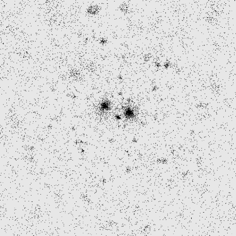
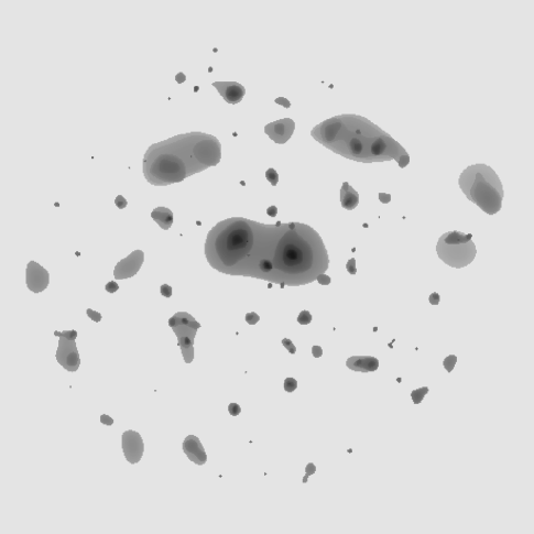
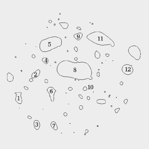
Figure 2.— Detection of extended sources in the 1701+6411 field. The wavelet decomposition uses the photon image (a) to detect significant structures of different angular scale (b). The wavelet image is split into a number of connected domains (c). The domains containing candidate extended sources are numbered. The best fit image is shown in panel d. Extended sources which passed our final selection are marked. All four sources were later confirmed as clusters by optical observations.

3.4. A Real-Life Example

To minimize computations, we fit the data only in those regions where the sum of scales 1–6 is positive, i.e. where an excess over the background is found by the wavelet decomposition. To improve the computational efficiency still further, the image is split into connected domains. Sources located within the same domain are fit simultaneously. The whole procedure of the extended source detection is illustrated in Fig 2. The raw photon image is shown in panel (a). The wavelet decomposition detects 97 sources in this field. The sum of scales 1–6 is shown in Fig 2b. This image is split into connected domains (Fig 2c). Domains which contain sources detected at scales 4, 5, or 6, are numbered. The best-fit model image in these domains is shown in Fig 2d. Extended sources which passed the final selection, are marked by arrows. All four of them are optically confirmed clusters. Note that the number of candidate extended sources found by the wavelet decomposition is more than 3 times the number of finally selected clusters. Thus, the selection of candidate sources by the wavelet analysis is rather lenient and does not miss real extended sources.

Using the detection procedure described in this section, we selected 239 significantly extended X-ray sources in 647 fields. In the following sections we describe the measurement of their X-ray parameters, optical observations, and present our final catalog.

4. Measurement of Cluster X-ray Parameters

For each detected cluster, we derive its position, radius, total X-ray flux, and their uncertainties. All these quantities are derived from the best-fit $\beta$-model, and their statistical errors are determined by Monte-Carlo simulations. For this, we use the best-fit model image (which includes clusters, point sources, and the background) as a template, simulate the data using Poisson scatter, and refit the simulated data. The errors are determined from the distribution of the best fit values in 100 simulations. In this section, we discuss the measurement details and sources of additional systematic errors of the cluster parameters.

4.1. Positional Accuracy

Cluster position is measured as the best-fit centroid of the $\beta$-model. In addition to the statistical uncertainty of the position, there is a systematic uncertainty due to inaccuracy of the ROSAT aspect solution. The aspect solution errors result in a systematic offset of all X-ray sources in the field with respect to their optical counterparts. To correct this error, we examined the positional correspondence of X-ray sources and objects in the Digitized Sky Survey (DSS). If possible, targets of observations or other prominent sources (galaxies or bright stars) were used to find the precise coordinate correction. Coordinate shifts measured this way have an uncertainty of 2″–5″, which is negligible compared to the statistical error of cluster positions. If no optical counterparts of X-ray sources were found in the DSS, we assigned a systematic position error of 17″, the rms value of shifts measured using targets of observation. In some observations without a bright target, we found a correlation between fainter X-ray and optical sources, and measured shifts from this correlation. We regarded this shift measurement as less reliable than that using targets, and assigned an intermediate systematic error of 10″ to the cluster position in such fields. The uncertain rotation of the PSPC coordinate system results in a systematic error of $\sim 5\arcsec$ or less (Briel et al. 1996). We did not correct for the rotation, but simply added $5\arcsec$ in quadrature to the offset uncertainty. The final position error listed in Table 2 is the sum of systematic and statistical errors in quadrature.

4.2. Core-Radius

Since it is impossible to fit the $\beta$-parameter using our data, we measure core-radius for fixed $\beta=0.67$ and refer to this value as the effective cluster radius $r_{e}$. Effective radius can be also defined as the radius at which the surface brightness falls by a factor of $2^{3/2}$ and hence is a physically meaningful combination of core-radius and $\beta$. The $r_{e}$ measurement by fitting a $\beta=0.67$ model is accurate to $\pm 20\%$ within the observed range of $\beta$, $0.6<\beta<0.8$ (Jones & Forman 1998).

We will now show that the radius measurement is relatively insensitive to the presence of cooling flows which cause a surface brightness excess in the central region of the cluster (e.g.  Fabian 1994). Cooling flow clusters in general cannot be fit by the $\beta$-model. However, in distant clusters, the cenral excess is completely removed by the PSF blurring, and cooling flows simply reduce the core-radius value. To study the possible influence of the cooling flow on the derived effective radii, we use the ROSAT PSPC image of Abell 2199, a nearby cluster with a moderate cooling flow of $200\,M_{\odot}\,$yr^-1 (Edge et al. 1992). The $\beta$-model fit for all radii yields $\beta=0.57$, $r_{c}=69\,$kpc. If the inner 200 kpc region is excluded to remove the cooling flow contamination, the best-fit parameters are $\beta=0.64$, $r_{c}=137\,$kpc, which corresponds to an effective radius of $142\,$kpc. We then determine the radius value which we would measure if A2199 were located at $z=0.4$. At this redshift, the FWHM of the PSF corresponds to $\sim 200$ kpc. We convolve the image with this “PSF” and fit accounting for the smoothing and without exclusion of the center. The best fit parameters for the smoothed data are $\beta=0.61$, $r_{c}=95\,$kpc. Fixing $\beta=0.67$, as we do for the analysis of distant clusters, we obtain $r_{c}=110$ kpc, only 22% smaller than the true value obtained by excluding the cooling flow.

4.3. X-ray Flux

The surface brightness of most of detected extended sources significantly exceeds the background only in a very limited area near the source center. Therefore, the total source flux simply integrated in a wide aperture has unacceptably large statistical uncertainty. To overcome this, the flux is usually directly measured within some small aperture, and then extrapolated to infinity using a reasonable model of the surface brightness profile (Henry et al. 1992, Nichol et al. 1997, Scharf et al. 1997). Similarly to this approach, we derived total fluxes from the normalization of the best fit $\beta$-model. The most serious problem with the flux measurement using such limited aperture photometry is the necessity to extrapolate the observed flux to infinity. This extrapolation is a potential source of large systematic errors because the surface brightness distribution at large radii is unknown. For example, consider the flux extrapolation from the inner 2.5 core radius region using $\beta$-models with different $\beta$. This inner region contains 49% of the total flux if $\beta=0.6$, 64% if $\beta=0.67$, and 70% if $\beta=0.7$. Therefore, assuming $\beta=0.67$ one underestimates the flux by $\sim 30\%$ if in fact $\beta=0.6$, the median value in the Jones & Forman (1998) sample. In addition, a trend of $\beta$ with cluster redshift or luminosity will introduce systematic changes within the sample. For example, Jones & Forman find that lower luminosity clusters have smaller $\beta$, which might result in underestimation of their fluxes.

To address the issue of systematic flux errors in more detail, we have used simulated realistic data (§7) to estimate the effect of the assumed value of $\beta$ on the cluster flux determination. Clusters were fit as described in §3.3, but for three different values of $\beta$, 0.6, $0.67$, and $0.7$. Dashed lines in Fig 4.3 show average ratios of the measured and input total flux as a function of the true $\beta$, if the flux is measured as a normalization of the best-fit model with $\beta$ fixed at 0.6 and 0.7. In all cases significant biases are present over the observed range of $\beta$ (Jones & Forman 1998; shaded region). We are interested in a flux measure which has the smallest uncertainty for the whole range of $\beta$, not the one which yields an unbiased flux estimate for some fixed value of $\beta$. The quantity $(f_{0.6}+f_{0.7})/2$, where $f_{0.6}$ and $f_{0.7}$ are cluster fluxes calculated assuming $\beta=0.6$ and $0.7$, respectively, is close to the desired flux measure (solid line in Fig 4.3). It provides a satisfactory flux estimate, accurate to $\pm 10\%$ over the observed range of $\beta$. We use this quantity to measure cluster fluxes throughout the rest of this paper, and add the systematic error of $10\%$ to the statistical uncertainty in the flux.

Table 1Comparison of flux measurements

Cluster	$z$	Our survey	EMSS	Nichol et al.	WARPS	Flux ratioa
		0.5–2 keV	0.3–3.5 keV	0.3–3.5 keV	0.5–2 keV	EMSS	Nichol et al.	WARPS
MS 1201.5+2824	0.167	102.6	169.4	174.7	95.6	1.03	1.00	1.07
MS 1208.7+3928	0.340	126.6	141.1	142.7	29.3	1.12	1.08	0.91
MS 1308.8+3244	0.245	146.7	169.3	174.9	50.7	1.16	1.07	0.92
MS 2255.7+2039	0.288	150.5	157.6	173.9	51.9	1.53	1.19	0.97
Average						1.21	1.09	0.97

^a Ratios of fluxes measured in our survey and EMSS, Nichol et al., and WARPS. To calculate these ratios, 0.3–3.5 keV fluxes were converted to the 0.5–2 keV energy band using the conversion coefficients from Jones et al. (1998).

Our sample includes four EMSS clusters (Henry et al. 1992), which were also detected in the WARPS survey (Jones et al. 1998) and whose ROSAT observations were studied by Nichol et al. (1997). We use these clusters to compare fluxes from all these surveys. Table 1 shows general agreement, within 10%, between different ROSAT surveys, especially between ours and WARPS. However, Henry et al. and, to a smaller degree, Nichol et al. find fluxes which are systematically lower than those from our survey and WARPS. Note that all ROSAT surveys use essentially the same data, so the difference cannot be explained by statistical fluctuations. Jones et al. have earlier performed a similar comparison using a larger number of clusters. They also noted the systematic difference of their fluxes compared to EMSS and Nichol et al., and explained this by the difference in flux measurement methods. All the surveys derived fluxes by extrapolation from that measured within some aperture using a $\beta$-model. However, Henry et al. and Nichol et al. assumed fixed $\beta=0.67$ and $r_{c}=250$ kpc, while Jones et al. estimated core-radii individually for each cluster, similar to our procedure. Also, our fluxes can be $\sim 5\%$ higher than those obtained for $\beta=0.67$, because our measurements are optimized for the entire observed range of $\beta$. Cluster-to-cluster variations of $\beta$ probably explain $\sim 10\%$ non-systematic differences in flux for the same cluster in different surveys. Jones et al. also compared their measurements with fluxes directly integrated in a 4 Mpc aperture. They found that their fluxes exceed the directly measured values by 10%, with $\sim 60\%$ of that difference explained by the cluster luminosity originating from outside 4 Mpc. Since our measurements are $\sim 3\%$ lower than those of Jones et al., we conclude that our fluxes are accurate within a few percent which is better than the assigned systematic uncertainty.

Ratio of the measured and input cluster flux as a function of the cluster $\beta$. Fluxes of simulated clusters were measured by fitting $\beta$-models with $\beta$ fixed at 0.6 (upper dashed line), 0.7 (lower dashed line) and 0.67 (dotted line). Solid line corresponds to the flux measure $(f_{0.6}+f_{0.7})/2$ used for our sample.

5. Optical observations

We are carrying on a program of optical photometric and spectroscopic observations of our clusters. A complete discussion of optical observations and data reduction will be presented in McNamara et al. (in preparation). Below we discuss the optical results relevant to the X-ray catalog presented here.

5.1. Cluster Identification

In some earlier works, optical identification of X-ray selected clusters seeks a concentration of galaxies in redshift space, which requires a large investment of telescope time. For our sources, the detected extended X-ray emission is already a strong indication of cluster existence. Therefore, we relaxed the optical identification criteria and required that either a significant enhancement in the projected density of galaxies be found or that an elliptical galaxy not included in the NGC catalog lie at the peak of the X-ray emission. While the galaxy concentration criterion is obvious, the elliptical galaxy one is needed to identify poor clusters and groups which fail to produce a significant excess of galaxies over the background. It also helps to identify “fossil groups”, in which galaxies have merged into a cD (Ponman et al. 1994). A potential problem with this second criterion is that an active nucleus of an elliptical galaxy might be falsely identified as a cluster. However, a significant extent of X-ray emission in all our sources makes this unlikely. Also, our spectroscopic observations of such single-galaxy sources never showed emission lines characteristic of AGNs.

Status of optical identifications

Total sample
Objects	223
Confirmed clusters	200
False X-ray detections	18
No CCD imaging data	5
NED identifications
Previously known clusters	37
Previously known clusters with measured redshift	29
NED AGN	1
X-ray flux $>2\times 10^{-13}\,$ergs s${}^{-1}\,$cm-2
Objects	82
Confirmed clusters	80
False detections	1
No data	1

We obtained R, and in some cases I, V, and B band CCD images on the FLWO 1.2m, Danish 1.54m, and Las Campanas 1m telescopes. For brighter clusters, we also used second generation Digitized Sky Survey (DSS-II) plates. Using the DSS-II, it is possible to identify clusters at $z\lesssim 0.45$. The sensitivity of our CCD images is adequate to identify clusters to $z=0.7-0.9$. If no cluster was visible in the CCD image, we considered this object as a false detection (although it could be a very distant cluster). These objects were retained in the sample for statistical completeness, but marked in Table 2.

We also searched for possible optical counterparts in the NASA Extragalactic Database (NED). The summary of NED identifications is given in Table 5.1. We obtained CCD photometry for some of the catalogued clusters and tried to obtain spectroscopic data if redshifts were not available. Fifteen extended sources were identified with isolated NGC galaxies, and therefore removed from the cluster catalog. One object, identified with an AGN, was considered as a false detection but was left in the catalog for statistical completeness.

A summary of optical identifications of our cluster catalog is given in Table 5.1. In total, we confirmed 90% of sources as clusters in the total sample, while 8% of sources are likely false detections. For 2% of sources, no optical counterpart was present in the DSS-II and no CCD images were yet obtained. In the X-ray bright subsample, $f>2\times 10^{-13}\,$ergs s${}^{-1}\,$cm^-2, we optically confirmed 98% of sources as clusters; one object in this subsample is a false detection and for the remaining one, optical images are saturated by neighboring Arcturus. These high success rates demonstrate the high quality of our X-ray selection.

Figure 3.— (a) X-ray luminosity corrected BCG magnitudes vs. redshift. The dotted line shows the analytical fit (see text). The estimated redshift uncertainty of $\Delta z=^{+0.04}_{-0.07}$ is shown by dashed lines. Crosses mark five high-redshift EMSS clusters. These clusters were not used in the fit. (b) Same as (a) but magnitudes were measured using DSS-II. The dotted line shows the best fit relation, and dashed lines correspond to $\Delta z=\pm 0.07$.

5.2. Spectroscopic and Photometric Redshifts

We observed an incomplete subsample of clusters spectroscopically on the MMT, ESO 3.6m, and Danish 1.54m telescope. In most cases, we identified several obvious cluster galaxies in the CCD images and then obtained a long-slit spectrum, usually for 2–3 galaxies per cluster. The slit always included the brightest cluster galaxy. For 10 clusters observed at the ESO 3.6m telscope, we obtained multi-object spectra, 10–15 galaxies per cluster. Altogether, we measured 47 redshifts ranging from $z=0.040$ to $z=0.574$. Further details of spectroscopic observations will be presented in McNamara et al. (1998, in preparation).

For those clusters without spectroscopic data, we estimated redshifts from the magnitude of the brightest cluster galaxy (BCG). The BCG was selected as the brightest galaxy either within the error circle of the cluster X-ray position or the one in the center of the galaxy concentration; both criteria were met simultaneously in most cases. Although the BCG selection was somewhat subjective, the tightness of the magnitude vs. redshift relation obtained for $\sim 1/4$ of the total sample confirms our procedures. For nearby clusters, the scatter in the absolute magnitude of BCGs is small, $\sigma_{M}\approx 0.2$ (Sandage 1972), which corresponds to $\approx 10\%$ distance error. Our results show that the scatter is small at higher redhifts as well. The magnitude vs. redshift relation is calibrated within our sample, and photometric redshifts are estimated using the CCD images obtained under photometric conditions or DSS-II plates.

The CCD galaxy photometry was performed in the R band. The BCG magnitudes were measured within a fixed 4″aperture. Such an aperture was chosen to make the measurement relatively insensitive to poor seeing, which was $\sim 2\arcsec$ in some cases, and encompass $\sim 50\%$ of light in high-redshift galaxies. The fixed angular aperture corresponds to the metric aperture increasing with redshift, from 10 kpc at $z=0.1$ to 29 kpc at $z=0.5$. The increase of the metric aperture is a monotonic function of redshift, the same for all clusters, and thus does not prevent us from using the $m-z$ relation for photometric redshift estimates. We did not make K-corrections of BCG magnitudes because this is also a monotonic systematic function of redshift. Measured magnitudes were corrected for Galactic extinction using Burstein & Heiles (1982) maps.

There is a correlation between the BCG magnitude and the cluster X-ray luminosity (Hudson & Ebeling 1997), which increases the scatter in the $m-z$ relation. Within our sample, the absolute BCG magnitude changes approximately as $-0.5\log L_{x}$, in good agreement with the Hudson & Ebeling results. Below we use the corresponding correction, $m^{\prime}=m+0.5\log(L_{x}/10^{44}\,\mbox{erg s${}^{-1}$})$ to compensate for this effect.

The X-ray luminosity-corrected BCG magnitude is plotted vs. cluster redshift in Fig 3. This dependence can be well fit by a cosmological dimming law $m^{\prime}=m_{0}+5\log z-1.086(q^{\prime}-1)z$ with best-fit parameters $m_{0}=20.45^{\rm m}$ and $q^{\prime}=-0.121$. In this equation, $q^{\prime}$ provides a useful parametrization but does not have the meaning of the cosmological deceleration parameter, because magnitudes were not K-corrected and a varying metric aperture was used. The best fit relation is shown by the dotted line in Fig. 3. Photometric redshifts were estimated from the analytical fit using the following iterative procedure. We estimated redshift from the uncorrected BCG magnitude. Using the estimated redshift, we calculated the X-ray luminosity, corrected the BCG magnitude as described above, and re-estimated $z$. The process was repeated until the estimated redshift converged. We checked this procedure by estimating photometric redshifts of clusters with measured redshifts. This comparison has shown that the photometric estimate is unbiased and has an uncertainty of $\Delta z=^{+0.04}_{-0.07}$.

We also observed five high-$z$ EMSS clusters (0302+1658, 0451.6–0305, 0015.9+1609, 1137.5+6625, and 1054.5–0321) to check the $m-z$ relation at high redshift using an external X-ray selected sample. These clusters are plotted by crosses in Fig. 3. They follow the relation defined by our sample very well. In addition, these five EMSS clusters are very X-ray luminous; their accordance with the $m-z$ relation confirms the validity of the X-ray luminosity correction we apply to BCG magnitudes.

For 13 clusters without photometric CCD data, redshifts were estimated using the Second Digitized Sky Survey plates. Photometric calibration of was performed using our CCD images, and will be described in McNamara et al. (1998, in preparation). BCG magnitudes were measured in a fixed angular aperture of 5″. No K-correction was applied. The X-ray luminosity corrected DSS-II magnitudes are plotted vs. redshift in Fig. 3. The $m-z$ relation can be fit by the relation $m=m_{0}+5\log z-1.086(q^{\prime}-1)z$ with best fit parameters $m_{0}=19.84$, $q^{\prime}=-1.23$ photometric redshifts were estimated using a procedure analogous to that for the CCD data. The comparison of the estimated and measured redshifts yields the accuracy of the photometric estimate of $\Delta z\approx\pm 0.07$.

6. The Catalog

Our cluster catalog is presented in Table 2. The object number is given in column 1. The coordinates (J2000.0) of the X-ray centroid are listed in columns 2 and 3. The total unabsorbed X-ray flux in the 0.5–2 keV energy band (observer frame) in units of $10^{-14}\,$ergs s${}^{-1}\,$cm^-2 and it uncertainty are listed in columns 4 and 5. Angular core-radius and its uncertainty are given in columns 6 and 7. Column 8 contains spectroscopic or photometric redshifts. The 90% confidence interval of the photometric redshift is given in column 9. Thirteen clusters for which the DSS was used for photometric redshift are marked by superscript in column 9. If redshift is spectroscopic, no error interval is given. Three clusters show clear concentrations of galaxies near the X-ray position, but the choice of BCG is uncertain because of the large cluster angular size. We do not list photometric redshifts for these clusters and mark them by “U” in the Notes column. Columns 10 lists 90% X-ray position error circle. Column 11 contains notes for individual clusters. In this column, we list the optical identifications from the literature. We also mark likely false detections by “F”.

Table 9 shows coordinates and exposures for the 647 analyzed ROSAT pointings. For a quick estimate of sensitivity in each field, one can use the listed exposure time and Fig 7.1. In this figure, we show the limiting flux, at which clusters are detected with a probability of $90\%$ for off-axis angles between 2′ and 17.5′.

7. Monte-Carlo Simulations of Cluster Detection

For a statistical analysis of our cluster catalog, the detection efficiency as a function of flux and extent, and measurement uncertainty is required. To derive these functions, we used extensive Monte-Carlo simulations described in this section.

7.1. Correcting for Selection Effects

The most direct way to compare theoretical models with our cluster catalog is to predict the number of clusters within some interval of measured fluxes and radii (and redshift) and then compare the prediction with the number of detected clusters in this interval. To predict the number of detected clusters, one needs to know the detection probability as a function of real cluster flux, $f$, and radius, $r_{c}$, and the distribution of measured values, $f_{m}$ and $r_{c,m}$, also as a function of $f$ and $r_{c}$. Using a theoretical model, one calculates the number of real clusters as a function of flux and radius, then multiplies this number by the detection probability, and then convolves it with the measurement scatter.

Since the detection algorithm for extended sources is rather complicated, the only method of deriving appropriate corrections is through Monte-Carlo simulations.

Approximate limiting flux, at which the cluster detection probability is 90% in the range of off-axis angles $2\arcmin-17.5\arcmin$, plotted vs. exposure time. Limiting fluxes for three values of cluster core-radius, $r_{c}=15\arcsec$, 30″, and 60″, are shown. Sensitivity is best for $r_{c}\approx 30\arcsec$ and declines for smaller and larger clusters.

7.2. What Affects the Cluster Detection?

In this section, we discuss the effects that influence the cluster detection process, and therefore should be included in Monte-Carlo simulations.

The first obvious effect is the degradation of the ROSAT angular resolution at large off-axis angles. Because of this degradation, a cluster with $r_{c}=20\arcsec$ is well-resolved on-axis where the FWHM of the PSF is 25″, but the same cluster is indistinguishable from a point source if located at an off-axis angle of 17′ where the PSF is 57″ (FWHM).

Point sources, which may lie in the vicinity of a cluster, reduce the efficiency of cluster detection and increase the measurement errors. Therefore, the simulations should include realistic spatial and flux distributions of point sources.

In addition, exposure time, Galactic absorption, and the average background level vary strongly among the analyzed ROSAT fields, and so does the probability to detect a cluster of given flux. Also, the background has to be modeled individually for each field, and cannot be assumed known in simulations.

To model all these effects, we simulate realistic ROSAT images containing point sources, insert clusters with known input parameters at random positions into the simulated images, and analyze these images identically to the real data. The selection functions are then derived from comparison of the numbers and parameters of input and detected clusters.

7.3. Simulating ROSAT Images without Clusters

We begin with point sources which are the major contributor to the X-ray background in the ROSAT band. To simulate source fluxes, we use the $\log N-\log S$ relation measured in the flux range of $1.2\times 10^{-15}-10^{-12}\,$ergs s${}^{-1}\,$cm^-2 (Vikhlinin et al. 1995). Fluxes are simulated using the extrapolation of $\log N-\log S$ in the range from $10^{-11}$ to $2.5\times 10^{-17}\,$ergs s${}^{-1}\,$cm^-2, where the integral emission of point sources saturates the X-ray background. Source positions are simulated either randomly or with a non-zero angular correlation function using a two-dimensional version of the Soneira & Peebles (1978) algorithm. After the source position is determined, we convert the flux to the number of detected photons using the exposure time at the source position, and the counts-to-flux conversion appropriate to a power law spectrum with $\Gamma=2$ and the actual Galactic absorption in the simulated field. The number of detected source photons is drawn from a Poisson distribution. The photon positions are simulated around the source position according to the PSF as a function of off-axis angle. Finally, we add a flat Poisson background (corrected for the exposure variations across the field) until the average background levels are equal in the simulated image and the corresponding real observation. This flat uniform component corresponds to truly diffuse backgrounds, such as foreground Galactic emission, scattered solar X-rays, and the particle background.

The images simulated according to the described procedure correctly reproduce fluxes and the spatial distribution of point sources, the average background level, and background fluctuations caused by undetected point sources and their possible angular correlation.

7.4. Simulations of clusters

The next step is to put a cluster of a given flux and angular size at a random position in the image. An elliptical $\beta$-model

$$I(x,y)=I_{0}\;\left(1+x^{2}/a_{x}^{2}+y^{2}/a_{y}^{2}\right)^{-3\beta+1/2},$$ (4)

was used for cluster brightness. Cluster $\beta$ parameters and axial ratios were randomly selected from the distribution observed in nearby clusters (Jones & Forman 1998, Mohr et al. 1995). To include the influence of edge effects arising because detected clusters must lie between off-axis angles of 2′–17.5′, cluster positions were simulated in the inner 18.5′ circle of the field of view. Cluster flux was converted to the number of detected photons using the local exposure and the counts-to-flux coefficient corresponding to a $T=5$ keV plasma spectrum and the Galactic absorption for the field. The cluster model was convolved with the PSF calculated for the given off-axis angle. Photons were simulated using a Poisson distribution around the model and added to the image.

Reducing simulated images identically to the real data, we derive the detection efficiency as a function of flux and effective radius. Effective radius is defined as the radius at which the radially-averaged surface brightness drops by a factor of $2^{3/2}$ (§4.2). The effective radius can be calculated from parameters in eq. 4 as

$$r_{e}=\sqrt{a_{x}a_{y}\left(2^{1.5/(3\beta-0.5)}-1\right)}.$$ (5)

In simulations, we verified that the detection probability indeed has very little dependence on the $\beta$-parameter and axial ratio and is determined by $r_{e}$ only.

7.5. Simulation Runs

Simulated images were reduced identically to the real data, i.e. we modeled the background (§2), detected candidate extended sources by the wavelet decomposition (§3.2), fitted these candidate sources and applied our final selection criteria (§3.3), and recorded parameters of input and detected clusters. Each of the 647 ROSAT fields was simulated 650 times. Radii and fluxes of input clusters were randomly distributed in the 5″–300″, $10^{-14}$–$3\times 10^{-12}\,$ergs s${}^{-1}\,$cm^-2 range.

To derive the distribution of false detections, we performed a separate set of simulations without putting clusters into simulated images. In this set of simulations, each field was simulated 50 times.

Simulations were performed with point sources distributed either randomly or with the angular correlation function measured by Vikhlinin & Forman (1995) for faint ROSAT sources. The spatial correlation of point source significantly increases the number of false detections (by a factor of 1.5), but has little or no effect on the detection probability of real clusters.

The simulation results were used to measure the cluster selection functions necessary for a statistical study of our catalog. These data are available in electronic publication on AAS CDROM and through the WWW page http://hea–www.harvard.edu/x–ray–clusters/.

Probability of cluster detection as a function of flux and core-radius. Contours correspond to the detection probabilities of 1, 5, 10, 20, 30, 40, 50, 60, 70, 80, 90, and 99%.

7.6. Results of Simulations: Detection Probability

The probability that a cluster with unabsorbed flux $f$ and radius $r_{e}$, whose position falls within 18.5′ of the center of one of the analyzed ROSAT fields will be detected, is shown in Fig. 7.5. This probability is normalized to the geometric area of the annulus in which detected clusters may be located (2′–17.5′). At a given flux, the detection probability is the highest for clusters with radii of $\sim 30\arcsec$. It gradually decreases for clusters with large radius, because their flux is distributed over the larger area, thus decreasing their statistical significance. The detection probability also decreases for compact clusters, because they become unresolved at large off-axis angles. This effect is important for clusters with angular core radii of $\lesssim 15\arcsec$. Even at $z=1$ this radius corresponds to 130 kpc, which is two times smaller than the core-radius of a typical rich cluster (250 kpc, Jones & Forman 1998). Therefore, cluster detection efficiency is limited mainly by the low number of photons, not by the resolution of the ROSAT PSPC.

The detection probability changes by less than 10% for clusters with axial ratios $<0.7$ compared to azimuthally symmetric clusters. This is caused by significant PSF smearing, which reduces the apparent ellipticity of distant clusters. Similarly, we have found no significant dependence of the detection probability on the value of the $\beta$-parameter.

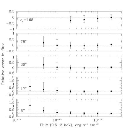
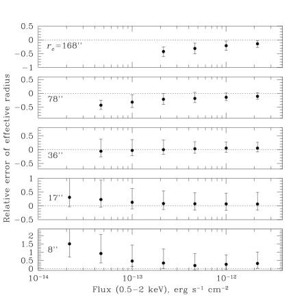
Figure 4.— Bias and scatter of flux and radius measurements. Points show the average relative deviation of the measured quantity. Error bars show the relative scatter of the measured quantity, not errors of bias.

Figure 5.— Distribution of false sources as a function of measured flux and radius (left), and a cumulative distribution as a function of flux (right). In the left panel, contours represent the levels of equal density of false source distribution. Contour labels show the number of false sources outside the contour. Points represent parameters of the likely false detections in the data, i.e. those X-ray sources which have no cluster counterparts in deep CCD images.

7.7. Results of Simulations: Measurement Scatter and Bias

In this section we consider the distribution of measured flux and radius of detected clusters, as a function of input flux and radius. This distribution is derived for clusters detected in any field and at any off-axis angle, and is different from the uncertainties listed in Table 2, which are determined only by the photon counting statistics. Fig. 4 shows the distributions derived for several values of input cluster flux and radius. The points in this figure represent the mean relative deviation of the observed parameter, while the error bars show the mean relative scatter (both positive and negative). Generally, the flux measurement is unbiased and has a small relative scatter of $\sim 20\%$. At low fluxes, where the detection probability decreases, the measured fluxes tend to be overestimated. This bias is naturally present whenever a flux measurement is performed near the detection threshold, and is not related to the particular detection algorithm. For example, a source with a true flux exactly equal to the detection threshold will be detected with 50% probability, and in all these cases the measured flux exceeds the true flux. Averaged over detections, the measured flux exceeds the true value. This flux bias should be accounted for in deriving the luminosity functions and the $\log N-\log S$ relation. On the other hand, for clusters with very large radii, the flux is underestimated, because the background is overestimated near broad clusters. This effect is important only for clusters at low redshifts which have large angular core radii.

The radii of very compact clusters are strongly overestimated on average, because such clusters can be detected as extended sources only if their measured radius is a positive fluctuation with respect to the true value, similar to the flux bias above. The measured radii of very broad clusters are underestimated because of the oversubtraction of the background. The sizes of distant clusters mostly fall in the range of $15\arcsec-1\arcmin$, where our radius measurements are unbiased. For example, a radius of 250 kpc corresponds to 45″ at $z=0.3$, 35″ at $z=0.5$, and 29″ at $z=1$. At $z<0.2$, 250 kpc corresponds to large angular radii and therefore measured sizes of large low-redshift clusters are underestimated.

7.8. Results of Simulation: False Detections

Because of the finite angular resolution of the ROSAT PSPC, closely located point sources can be falsely classified as a single extended source. Optical identification is the most direct way of finding such false detections. However, optical observations alone, with no estimate of the number of false detections, could result in our failure to identify interesting new classes of objects such as quasars lensed by “dark” clusters (Hattori et al. 1997), clusters dominated by a single galaxy (Ponman et al. 1994), “failed” clusters (Tucker, Tananbaum, & Remillard 1995). Therefore, it is desirable to have an independent estimate of the number of false detections and their distribution as a function of flux and radius. For this, we simulate ROSAT images without clusters and reduce them identically to the real data. All the extended sources detected in these simulations are false. Since the simulations correctly reproduce fluxes and spatial distribution of point sources and all the instrumental artifacts of the ROSAT PSPC, the expected number of false detections can be accurately measured.

Confusion of point sources is the main effect leading to false cluster detections. The degree of confusion depends strongly on whether point sources are distributed randomly or have angular correlation, and the number of false detections changes correspondingly. From simulations, we derive that our source catalog should on average contain 17.2 false detections if point sources are randomly located. If point sources have correlation with the observed amplitude (Vikhlinin & Forman 1995), the number of false detections increases to 25.9. Fig 5 shows the distribution of false detections in radius vs. flux coordinates and their cumulative distribution as a function of flux, obtained for correlated point sources. For randomly located sources, the distributions in Fig 5 should simply be scaled. The contamination of our extended source catalog by confused point sources is between 8% and 11%.

The predicted number of false detections agrees well with results of optical identifications. From simulations, we expect on average $\approx 1.5$ false detections with fluxes $>2\times 10^{-13}\,$ergs s${}^{-1}\,$cm^-2. Of 82 X-ray sources above this flux, 80 are optically confirmed clusters, and one is a likely false detection. In the total sample, we expect $\approx 17-26$ false sources, while the presently available optical identifications set an upper limit of 23 and lower limit of 18 false detections in the data (Table 5.1). Finally, the distribution of flux and core-radius of X-ray sources without optical cluster counterparts matches well the distribution for false detections found in simulations (Fig 5). Thus, our sample provides no support for the existence of “dark” clusters.

7.9. Sky Coverage as a Function of Flux

To compute the $\log N-\log S$ function, the survey solid angle as a function of flux is required. Traditionally, the sky coverage is thought of as the area, in which a survey is “complete”, i.e. all sources above the given flux are detected. The differential $\log N-\log S$ is computed as the ratio of the number of detected sources in a given flux bin and the sky coverage in this flux bin. However, this view of the sky coverage is not correct in the presence of significant flux measurement errors, which is the case in all ROSAT surveys. First, the source detection probability changes gradually from 0 to 1 in a flux range of finite width, and cannot be adequately approximated by a step-like function of flux. Second, the measurement scatter leads to significant biases in the derived $\log N-\log S$ relation, as we describe below. Some intrinsically bright sources have low measured fluxes, while some intrinsically faint sources have high measured fluxes. For surveys with uniform sensitivity, the number of sources usually increases at faint fluxes and the described effect leads to overestimation of $\log N-\log S$ (Eddington 1940). In X-ray surveys, the sky coverage usually drops rapidly at faint fluxes and therefore the number of detected sources decreases at faint fluxes. In this case, the sign of the Eddington bias is opposite and the $\log N-\log S$ function is underestimated (see Fig. 6 in Hasinger et al. 1993a).

Sky coverage of the survey

Limiting Flux	Solid Angle (deg2)
ergs s${}^{-1}\,$cm-2	entire sample	$z>0.5$ clusters
$1.3\times 10^{-14}$	0.074	0.070
$1.5\times 10^{-14}$	0.094	0.089
$2.0\times 10^{-14}$	0.185	0.190
$3.0\times 10^{-14}$	1.354	1.364
$4.5\times 10^{-14}$	9.026	9.100
$7.0\times 10^{-14}$	34.74	34.03
$1.0\times 10^{-13}$	66.55	66.20
$1.5\times 10^{-13}$	102.6	104.3
$2.0\times 10^{-13}$	122.8	127.4
$3.0\times 10^{-13}$	140.9	147.0
$4.5\times 10^{-13}$	148.1	154.0
$7.0\times 10^{-13}$	149.3	159.6
$1.0\times 10^{-12}$	151.1	161.3
$1.5\times 10^{-12}$	157.1	164.7
$2.0\times 10^{-12}$	158.5	165.1

For a plausible model of the source population, one can calculate the ratio of the differential $\log N-\log S$ for detected and real sources, if the detection probability and measurement scatter is known. The ratio of these $\log N-\log S$ functions has the usual meaning of the sky coverage. This approach to the survey area calculation was used by Vikhlinin et al. (1995 and 1995b) to obtain an unbiased measurement of the $\log N-\log S$ relation for point sources. We use the same approach here to define the survey area for the present cluster survey. We assume non-evolving clusters with the luminosity function of Ebeling et al. (1997) in a $q_{0}=0.5$ cosmology. The distribution of cluster radii and their correlation with luminosities is adopted from Jones & Forman (1998). We simulate cluster redshifts between $z=0$ and $z=2$ using the cosmological volume-per-redshift law (e.g. Peebles 1993). We then simulate the rest-frame luminosity between $L_{x}=10^{42}$ and $10^{46}\,$ergs s^-1. Cluster radius is simulated from the distribution corresponding to the simulated luminosity. We then calculate the observed angular radius and flux accounting for the correlation between X-ray luminosity and temperature (e.g., David et al. 1993), the probability to detect this cluster (§7.6), and finally we simulate the measured flux (§7.7). The detection probability is added to the distribution of detected clusters as a function of measured flux, and 1 is added to the the number of input clusters in the corresponding bin of real flux. Simulating $10^{6}$ clusters according to this procedure, we determine the sky coverage as the ratio of detected and input sources in the corresponding flux bins. The calculated survey area is shown in Table 7.9. In this table we also show the sky coverage for the distant, $z>0.5$, subsample. The sky coverage for distant subsamples differs from that for the entire sample because of the different distribution of angular sizes.

Using different cluster evolution models (including evolution of luminosities, number density, and radii), we verified that the derived sky coverage varies by no more than $10\%$ compared to the no-evolution assumption, if cluster radii do not evolve. Using the present cluster sample, Vikhlinin et al. (1998) show that the distribution of sizes of distant and nearby clusters is indeed very similar.

Cluster $\log N-\log S$ relation. The results from our survey are shown as the heavy solid histogram with several individual points including error bars. Vertical error bars represent the uncertainty in the number of clusters, while horizontal error bars correspond to a possible systematic uncertainty in flux (§4.3). Other surveys are shown for comparison.

8. ${\rm LOG}\;N-{\rm LOG}\;S$  relation for clusters

Using the survey solid angle, we calculate the $\log N-\log S$ relation for clusters. Each optically confirmed cluster is added to the cumulative distribution with the weight equal to the inverse solid angle corresponding to its measured flux. The derived cumulative $\log N-\log S$ function is shown in Fig 7.9. We also show the cluster counts derived in other surveys: EMSS (adopted from Jones et al. 1998), ROSAT All-Sky survey sample of X-ray brightest clusters (BCS; Ebeling et al. 1997), WARPS survey (Jones et al. 1998), Rosati et al. (1998 and 1995), and an ultra-deep UK ROSAT survey (McHardy et al. 1997). The $\log N-\log S$ relation derived from our survey spans more than 2.5 orders of magnitude in flux. At the bright end, our result shows excellent agreement with the samples of nearby clusters from the BCS and EMSS. At intermediate fluxes, around $2\times 10^{-13}\,$ergs s${}^{-1}\,$cm^-2, our cluster counts agree well with a small-area WARPS survey. Finally, the extrapolation of our $\log N-\log S$ relation down to $3\times 10^{-15}\,$ergs s${}^{-1}\,$cm^-2, agrees with results of McHardy et al. (1997), who identified most of the X-ray sources, regardless of extent, in their ultra-deep survey. Our $\log N-\log S$ relation seems to be systematically higher than the surface density of clusters identified in the 50 deg² survey of Rosati et al. For example, the difference is a factor of 1.3 at $2\times 10^{-13}\,$ergs s${}^{-1}\,$cm^-2, where we optically confirmed 98% of detected sources and where the survey area corrections are relatively small. This difference is marginally significant at the $\sim 2\sigma$ level. Since Rosati et al. have not published their cluster sample nor the details of the survey area calculations, it is hard to assess the source of this discrepancy. We only note that it can be explained, for example, if there is a systematic difference of 15–20% in fluxes. A discrepancy of our $\log N-\log S$ relation with the EMSS near their sensitivity limit is most likely due to the difference in measured fluxes (§4.3).

9. Summary

We present a catalog of 200 clusters detected as extended X-ray sources in 647 ROSAT PSPC observations covering a solid angle of 158 square degrees. To detect these sources, we used a novel detection algorithm combining a wavelet decomposition to find candidate extended sources and Maximum Likelihood fitting to evaluate the statistical significance of the source extent. Optical identifications demonstrate a high success rate of our X-ray selection: 90% of detected sources in the total sample, and 98% in the bright subsample are optically confirmed as clusters of galaxies. We present X-ray parameters of all detected sources and spectroscopic or photometric redshifts for optically confirmed clusters. Extensive Monte-Carlo simulations of our source detections are used to derive the sky coverage of the survey necessary for a statistical study of X-ray properties of our clusters. We present the $\log N-\log S$ relation derived from our cluster catalog. This relation shows a general agreement with other, smaller area surveys.

In a subsequent paper (Vikhlinin et al. 1998) we use this sample to constrain the evolution of cluster luminosities and radii at high redshift.

Table 2Cluster catalog

No.	RA	DDec	$F_{x}$	$\delta F_{x}$	$r_{c}$	$\delta r_{c}$		$z$	$z_{\rm min}-z_{\rm max}$		$\delta r$	Note
	(J2000)	D(J2000)	$10^{-14}$ cgs		(″)	(″)					(″)
1	00  30  33.2	$+$26  18  19	24.3	3.0	31	3		0.500			13
2	00  41  10.3	$-$23  39  33	9.8	2.4	25	12		0.15	0.08–0.22dss		19
3	00  50  59.2	$-$09  29  12	36.6	4.9	45	4		0.21	0.14–0.25		11
4	00  54  02.8	$-$28  23  58	10.8	1.5	37	6		0.25	0.18–0.29		16
5	00  56  55.8	$-$22  13  53	25.9	5.2	61	12		0.11	0.04–0.18dss		17
6	00  56  56.1	$-$27  40  12	6.9	0.8	14	2		0.563			13	1
7	00  57  24.2	$-$26  16  45	186.1	21.3	82	6		0.113			14	2
8	01  10  18.0	$+$19  38  23	7.8	1.6	35	8		0.24	0.17–0.28		16
9	01  11  36.6	$-$38  11  12	8.9	1.7	18	3		0.122			9
10	01  22  35.9	$-$28  32  03	26.9	6.3	37	16		0.24	0.17–0.28		14	3
11	01  24  35.1	$+$04  00  49	7.5	2.2	31	14		0.27	0.20–0.31		20
12	01  27  27.8	$-$43  26  13	5.7	1.9	34	13		—3			19	F
13	01  28  36.9	$-$43  24  57	7.5	1.3	10	3		0.26	0.19–0.30		9
14	01  32  54.7	$-$42  59  52	32.3	8.1	75	25		0.088			23	4
15	01  36  24.2	$-$18  11  59	4.8	1.0	21	8		0.25	0.18–0.29		15
16	01  39  39.5	$+$01  19  27	10.9	2.0	37	8		0.25	0.18–0.29		12
17	01  39  54.3	$+$18  10  00	27.3	3.8	33	5		0.176			9	5
18	01  42  50.6	$+$20  25  16	26.1	4.5	29	6		0.43	0.36–0.47		22
19	01  44  29.1	$+$02  12  37	10.1	2.3	32	11		0.15	0.08–0.19		13
20	01  54  14.8	$-$59  37  48	14.5	3.2	22	7		0.360			12
21	01  59  18.2	$+$00  30  12	32.7	4.1	13	2		0.26	0.19–0.30		9
22	02  06  23.4	$+$15  11  16	13.0	2.5	53	10		0.27	0.20–0.31		14
23	02  06  49.5	$-$13  09  04	26.0	4.4	28	8		0.31	0.24–0.35		15
24	02  10  13.8	$-$39  32  51	4.6	1.1	22	10		0.19	0.12–0.23		11
25	02  10  25.6	$-$39  29  47	6.4	1.3	28	9		0.27	0.20–0.30		14
26	02  28  13.2	$-$10  05  40	24.4	3.9	35	6		0.149			15
27	02  36  05.2	$-$52  25  03	5.8	1.2	16	4		0.60	0.53–0.67dss		9
28	02  37  59.2	$-$52  24  40	64.4	8.2	49	8		0.13	0.06–0.20dss		14	6
29	02  39  52.6	$-$23  20  35	8.4	1.8	51	14		0.49	0.42–0.53		23
30	02  58  46.1	$+$00  12  44	10.8	2.9	28	7		0.23	0.16–0.27		19
31	02  59  33.9	$+$00  13  47	32.4	5.2	42	11		0.17	0.10–0.21		12
32	03  22  20.1	$-$49  18  40	40.3	7.2	69	11		0.067			15	7
33	03  37  44.9	$-$25  22  39	3.7	0.7	7	2		0.38	0.31–0.42		8
34	03  41  57.1	$-$45  00  11	1.7	0.4	27	9		0.36	0.29–0.43dss		12
35	03  51  37.8	$-$36  49  50	8.8	2.2	31	17		$\cdots$	$\cdots$		24	f?
36	04  28  43.0	$-$38  05  54	20.8	5.0	54	13		0.154			20	8
37	04  34  15.7	$-$08  31  17	7.2	2.2	25	14		0.24	0.17–0.28		24
38	05  05  57.8	$-$28  25  47	14.2	1.9	25	4		0.131			15
39	05  06  03.7	$-$28  40  44	19.5	3.4	84	20		0.11	0.04–0.18dss		21
40	05  21  10.7	$-$25  30  44	17.6	4.0	37	13		$\cdots$	$\cdots$		15
41	05  22  14.2	$-$36  25  04	18.4	3.8	16	5		0.54	0.47–0.61dss		9
42	05  28  40.3	$-$32  51  38	19.9	2.5	26	3		0.273			8
43	05  29  38.4	$-$58  48  10	5.6	1.0	10	3		$\cdots$	$\cdots$		9	f?
44	05  32  43.7	$-$46  14  11	41.1	4.3	12	1		0.10	0.03–0.17dss		7
45	05  33  53.2	$-$57  46  52	22.2	6.1	81	28		0.15	0.08–0.22dss		37
46	05  33  55.9	$-$58  09  16	9.0	2.8	53	20		$\cdots$	$\cdots$		30	f?
47	08  10  23.9	$+$42  16  24	238.6	27.2	59	5		0.064			14
48	08  18  57.8	$+$56  54  34	10.1	2.5	29	9		0.260			17
49	08  19  22.6	$+$70  54  48	10.1	1.8	24	6		0.226			15
50	08  19  54.4	$+$56  34  35	30.8	5.0	16	5		0.260			14
51	08  20  26.4	$+$56  45  22	22.9	4.2	39	14		0.043			18
52	08  26  06.4	$+$26  25  47	10.9	2.6	59	19		0.351			22
53	08  26  29.7	$+$31  25  15	11.1	4.7	47	22		0.26	0.19–0.30		31
54	08  31  16.0	$+$49  05  06	12.3	4.0	30	15		—3			17	F
55	08  34  27.4	$+$19  33  24	8.3	1.7	31	7		—3			18	F
56	08  41  07.4	$+$64  22  43	29.1	3.2	35	3		0.36	0.29–0.40		8
57	08  41  43.4	$+$70  46  53	8.9	2.1	31	12		0.235			13
58	08  42  52.8	$+$50  23  16	6.3	1.7	23	10		0.48	0.41–0.53		16
59	08  47  11.3	$+$34  49  16	12.2	3.0	28	9		0.560			17
60	08  48  47.6	$+$44  56  21	3.3	0.6	14	4		0.574			13
61	08  48  56.3	$+$44  52  16	2.7	0.6	23	6		—3			14	F
62	08  49  11.1	$+$37  31  25	14.7	3.0	36	10		0.240			14
63	08  52  33.6	$+$16  18  08	37.1	6.2	33	10		0.098			19
64	08  53  14.1	$+$57  59  39	19.8	5.8	35	14		0.475			17
65	08  57  45.7	$+$27  47  32	6.8	1.6	42	11		0.50	0.43–0.54		27
66	08  58  25.0	$+$13  57  16	6.4	1.0	14	5		0.54	0.47–0.58		10
67	09  07  17.9	$+$33  30  09	4.4	0.8	24	5		0.46	0.39–0.49		14
68	09  07  20.4	$+$16  39  09	148.5	17.6	55	5		0.076			9	9
69	09  10  39.7	$+$42  48  41	8.3	2.0	76	23		$\cdots$	$\cdots$		24	U
70	09  21  13.4	$+$45  28  50	23.9	4.7	26	5		0.337			11
71	09  26  36.6	$+$12  42  56	16.7	2.1	16	3		0.50	0.43–0.54		9
72	09  26  45.6	$+$12  34  07	11.7	3.5	60	22		—3			41	F
73	09  43  32.2	$+$16  40  02	23.1	3.7	36	5		0.256			10
74	09  43  44.7	$+$16  44  20	21.2	4.1	69	13		0.180			17
75	09  47  45.8	$+$07  41  18	13.5	3.7	32	10		0.59	0.52–0.63		17
76	09  51  47.0	$-$01  28  33	7.1	1.9	25	11		0.53	0.46–0.57		22
77	09  52  08.7	$-$01  48  18	9.3	2.5	39	14		—3			18	F
78	09  53  31.2	$+$47  58  57	13.0	5.2	41	20		—3			20	F, 10
79	09  56  03.4	$+$41  07  14	15.6	3.3	13	6		0.73	0.66–0.77		13
80	09  57  53.2	$+$65  34  30	9.4	1.7	19	5		0.530			12
81	09  58  13.5	$+$55  16  01	48.2	7.1	67	14		0.20	0.12–0.23		15	11
82	09  59  27.7	$+$46  33  57	10.5	5.2	37	23		—3			31	F
83	10  02  40.4	$-$08  08  46	8.6	2.1	29	7		0.62	0.55–0.66		12
84	10  10  14.7	$+$54  30  18	21.0	2.9	20	4		0.045			14	12
85	10  11  05.1	$+$53  39  27	4.7	1.2	23	9		0.30	0.23–0.34		11
86	10  11  26.0	$+$54  50  08	20.0	5.1	94	22		0.294			24
87	10  13  38.4	$+$49  33  07	45.6	9.8	107	21		0.17	0.10–0.21		22
88	10  15  08.5	$+$49  31  32	10.8	2.6	14	8		0.45	0.38–0.49		10
89	10  33  51.9	$+$57  03  10	14.5	4.3	24	9		0.06	0.00–0.10		16
90	10  36  11.3	$+$57  13  31	18.8	3.9	15	6		0.31	0.24–0.35		13
91	10  48  00.1	$-$11  24  07	18.5	3.6	35	7		0.065			19
92	10  49  02.7	$+$54  24  00	9.1	1.6	22	9		0.20	0.13–0.24		12
93	10  53  18.4	$+$57  20  47	2.5	0.3	12	3		0.340			8	13
94	10  56  12.6	$+$49  33  11	12.9	1.9	64	15		0.199			23
95	10  58  13.0	$+$01  36  57	129.5	19.3	113	13		0.038			15	14
96	11  17  12.0	$+$17  44  24	12.0	5.6	65	33		0.51	0.44–0.55		26
97	11  17  26.1	$+$07  43  35	6.1	1.6	18	7		0.40	0.33–0.44		12
98	11  17  30.2	$+$17  44  44	14.4	2.5	36	10		0.63	0.56–0.67		16
99	11  19  43.5	$+$21  26  44	5.5	0.9	12	3		0.11	0.04–0.15		9
100	11  20  57.9	$+$23  26  41	21.3	5.0	29	8		0.71	0.64–0.75		16
101	11  23  10.2	$+$14  09  44	18.2	4.9	49	24		0.32	0.25–0.36		27
102	11  24  03.8	$-$17  00  11	10.8	3.4	34	19		0.41	0.34–0.45		22
103	11  24  36.9	$+$41  55  59	40.1	9.6	110	30		0.18	0.11–0.22		31
104	11  35  54.5	$+$21  31  05	17.8	4.0	72	20		0.14	0.07–0.18		17
105	11  38  43.9	$+$03  15  38	15.9	3.7	18	6		0.14	0.07–0.18		10
106	11  42  04.6	$+$21  44  57	45.9	17.4	56	34		0.18	0.11–0.22		26
107	11  46  26.9	$+$28  54  15	39.2	5.8	79	11		0.17	0.10–0.21		18
108	11  51  40.3	$+$81  04  38	3.7	1.1	27	7		0.27	0.20–0.31		14
109	11  58  11.7	$+$55  21  45	4.7	1.0	21	5		0.15	0.08–0.19		9
110	11  59  51.2	$+$55  31  56	74.2	7.6	24	2		0.081			7	15
111	12  00  49.7	$-$03  27  31	18.5	2.6	29	5		0.39	0.32–0.42		10
112	12  04  04.0	$+$28  07  08	102.6	11.4	32	3		0.167			7	16
113	12  04  22.9	$-$03  50  55	8.7	1.3	26	6		0.22	0.15–0.26		14
114	12  06  33.5	$-$07  44  28	129.0	16.3	64	7		0.12	0.05–0.16		15
115	12  11  15.3	$+$39  11  38	26.6	3.8	14	4		0.340			8	17
116	12  13  35.3	$+$02  53  26	14.3	3.0	27	9		0.39	0.32–0.43		13
117	12  16  19.4	$+$26  33  26	15.4	4.2	15	6		0.428			15
118	12  18  29.1	$+$30  11  46	5.3	1.4	18	9		0.33	0.26–0.37		11
119	12  21  24.5	$+$49  18  13	20.6	4.6	34	8		0.70	0.64–0.74		18
120	12  22  32.5	$+$04  12  02	6.3	1.6	15	7		—3			12	F
121	12  36  31.4	$+$00  51  43	4.8	1.2	28	8		0.17	0.10–0.21		14
122	12  37  25.1	$+$11  41  27	10.6	3.4	41	15		$\cdots$	$\cdots$		21	U
123	12  37  38.6	$+$26  32  23	7.0	2.3	31	12		0.28	0.21–0.33		14
124	12  52  05.4	$-$29  20  46	21.7	4.2	46	11		0.17	0.10–0.21		13
125	12  52  11.3	$-$29  14  59	8.7	1.6	11	5		—3			8	F
126	12  54  38.3	$+$25  45  13	10.2	2.0	31	7		0.193			13
127	12  54  53.6	$+$25  50  55	13.2	2.5	40	8		0.23	0.16–0.27		12
128	12  56  04.9	$+$25  56  52	9.9	1.9	30	7		0.17	0.10–0.21		11
129	12  56  39.4	$+$47  15  19	5.7	0.8	25	5		0.40	0.33–0.44		10
130	13  01  43.6	$+$10  59  33	28.1	5.6	54	11		0.30	0.23–0.34		18
131	13  09  55.6	$+$32  22  31	9.0	2.9	42	19		0.290			23
132	13  11  12.8	$+$32  28  58	46.7	5.8	22	3		0.245			8	18
133	13  11  30.2	$-$05  51  26	13.7	2.4	36	6		0.49	0.42–0.53		20
134	13  25  14.9	$+$65  50  29	10.1	3.1	54	21		0.180			28
135	13  25  43.9	$-$29  43  51	7.7	2.7	43	11		—3			17	F
136	13  29  27.3	$+$11  43  31	97.0	16.6	120	16		0.023			22	19
137	13  34  31.1	$-$08  22  29	5.2	1.1	13	5		—3			10	F
138	13  34  34.4	$+$37  56  58	1.6	0.3	16	5		0.308			11	20
139	13  35  03.7	$+$37  50  00	2.9	0.4	21	4		0.382			9	21
140	13  36  42.1	$+$38  37  32	5.9	1.6	20	9		0.180			16
141	13  37  48.3	$+$48  15  46	7.1	1.5	16	4		—3			10	F
142	13  37  50.4	$+$26  38  49	9.6	2.1	21	6		0.28	0.21–0.33		12
143	13  37  53.3	$+$38  54  09	14.3	3.6	32	9		0.29	0.22–0.33		17
144	13  40  33.5	$+$40  17  47	16.1	2.5	19	5		0.171			10	22
145	13  40  53.7	$+$39  58  11	34.4	6.9	66	16		0.169			19	23
146	13  41  51.7	$+$26  22  54	814.0	84.6	103	4		0.070			8	24
147	13  42  05.0	$+$52  00  37	12.4	1.9	10	4		—3			13	F
148	13  42  49.1	$+$40  28  11	7.4	2.0	15	6		0.53	0.46–0.57		16
149	13  43  25.0	$+$40  53  14	12.6	2.8	18	7		0.140			10
150	13  43  29.0	$+$55  47  17	17.5	2.8	109	17		0.11	0.04–0.18dss		23
151	13  54  16.9	$-$02  21  47	14.5	2.6	27	4		0.49	0.42–0.53		11
152	13  54  49.1	$+$69  17  20	6.4	1.9	26	10		0.18	0.11–0.22		15
153	14  06  16.3	$+$28  30  52	8.5	1.2	14	4		0.546			9
154	14  06  54.9	$+$28  34  17	25.7	3.2	30	3		0.118			8
155	14  10  12.4	$+$59  42  40	33.5	5.1	38	12		0.249			18
156	14  10  15.2	$+$59  38  31	20.1	8.7	31	22		0.249			17	25
157	14  15  37.9	$+$19  06  33	25.4	3.4	52	5		$\cdots$	$\cdots$		13	26
158	14  16  28.7	$+$44  46  41	40.4	5.2	16	4		0.400			8
159	14  18  31.1	$+$25  10  50	75.6	7.8	33	1		0.24	0.17–0.28		7
160	14  18  45.2	$+$06  44  02	16.4	3.0	18	5		—3			9	F
161	14  19  23.5	$+$06  38  42	13.1	1.9	17	4		0.61	0.54–0.65		9
162	14  19  57.2	$+$06  34  26	10.3	2.1	35	7		0.61	0.54–0.65		15
163	14  29  38.1	$+$42  34  25	8.5	2.4	35	12		0.30	0.23–0.34		26
164	14  38  55.5	$+$64  23  44	26.2	3.6	103	11		$\cdots$	$\cdots$		19	U
165	14  44  07.7	$+$63  44  58	17.4	3.2	26	9		0.298			15	27
166	15  00  02.7	$+$22  33  51	14.5	4.5	37	17		0.21	0.14–0.25		24
167	15  00  51.5	$+$22  44  41	17.8	4.2	31	10		0.450			16
168	15  15  32.5	$+$43  46  39	34.6	9.7	60	19		0.26	0.19–0.30		18
169	15  15  36.8	$+$43  50  50	10.5	3.8	34	18		0.14	0.07–0.18		22
170	15  24  40.3	$+$09  57  39	30.4	4.1	26	3		0.11	0.04–0.15		9	28
171	15  37  44.3	$+$12  00  26	26.4	7.4	84	26		0.15	0.08–0.19		30
172	15  40  53.3	$+$14  45  34	7.6	2.0	17	8		0.45	0.38–0.49		13
173	15  44  05.0	$+$53  46  27	9.7	2.2	35	11		0.33	0.26–0.37		19
174	15  47  20.7	$+$20  56  50	25.4	7.0	51	20		0.23	0.17–0.28		24
175	15  52  12.3	$+$20  13  45	49.5	6.0	59	7		0.136			9
176	16  06  42.5	$+$23  29  00	12.1	2.8	34	13		0.310			12
177	16  20  22.0	$+$17  23  05	20.8	3.7	35	8		0.112			12
178	16  29  46.1	$+$21  23  54	25.3	4.0	46	8		0.184			19
179	16  30  15.2	$+$24  34  59	179.4	25.9	129	13		0.09	0.02–0.13		23	29
180	16  31  04.6	$+$21  22  02	29.1	6.4	58	14		0.098			16
181	16  33  40.0	$+$57  14  37	3.5	0.7	24	8		0.239			14
182	16  39  55.6	$+$53  47  56	130.5	14.8	170	8		0.111			12	30
183	16  41  10.0	$+$82  32  27	80.5	10.9	78	11		0.26	0.19–0.30		13	31
184	16  41  52.5	$+$40  01  29	29.4	7.8	51	15		0.51	0.44–0.55		24
185	16  42  33.5	$+$39  59  05	5.3	1.4	19	9		—3			12	F, 32
186	16  42  38.9	$+$39  35  53	10.1	2.3	27	9		0.47	0.40–0.51		16
187	16  58  34.7	$+$34  30  12	33.6	5.2	58	10		0.330			16
188	16  59  44.6	$+$34  10  17	9.8	3.4	25	11		0.32	0.25–0.36		16
189	17  00  42.3	$+$64  13  00	45.6	4.7	18	1		0.225			7	33
190	17  01  23.0	$+$64  14  11	38.6	4.2	25	2		0.453			7
191	17  01  46.1	$+$64  21  15	3.5	0.7	32	8		0.220			14
192	17  02  13.3	$+$64  20  00	6.3	1.2	32	7		0.224			12
193	17  22  53.8	$+$41  05  25	29.4	6.5	42	12		0.33	0.26–0.37		22
194	17  29  01.9	$+$74  40  46	17.3	7.2	100	31		0.28	0.21–0.35dss		40
195	17  46  29.1	$+$68  48  54	22.3	3.2	56	10		0.217			13
196	20  03  28.4	$-$55  56  47	47.6	6.3	16	2		0.015			8	34
197	20  04  49.4	$-$56  03  44	10.4	2.5	30	11		0.71	0.64–0.78dss		16
198	20  05  13.6	$-$56  12  58	35.0	4.9	7	3		—3			9	F
199	20  59  55.2	$-$42  45  33	11.2	1.8	9	3		0.47	0.40–0.51		8
200	21  08  51.2	$-$05  16  49	11.6	1.7	34	7		0.30	0.23–0.34		12
201	21  14  20.4	$-$68  00  56	25.8	3.3	17	3		0.15	0.08–0.19		13
202	21  37  06.7	$+$00  26  51	27.8	5.7	55	20		0.05	0.00–0.12dss		21	35
203	21  39  58.5	$-$43  05  14	8.3	2.0	12	6		0.30	0.23–0.34		15
204	21  46  04.8	$+$04  23  19	13.8	2.1	17	2		0.531			13
205	22  02  44.9	$-$19  02  10	6.6	2.2	36	9		0.34	0.27–0.38		22
206	22  12  38.2	$-$17  13  55	5.4	1.4	22	13		0.12	0.05–0.16		12
207	22  13  31.0	$-$16  56  11	18.1	3.2	41	12		0.32	0.25–0.36		17
208	22  39  24.7	$-$05  47  04	22.2	3.5	11	2		0.245			13	36
209	22  39  34.4	$-$06  00  14	5.9	2.0	21	10		0.15	0.08–0.19		19
210	22  39  38.9	$-$05  43  18	32.4	5.0	34	5		0.245			15	37
211	22  47  29.1	$+$03  37  13	23.0	6.3	46	17		0.18	0.11–0.22		20
212	22  57  49.4	$+$20  56  25	11.1	2.1	22	7		0.28	0.21–0.32		11
213	22  58  07.1	$+$20  55  07	50.5	6.1	24	3		0.288			9	38
214	23  05  26.2	$-$35  46  01	15.5	3.4	55	14		0.21	0.14–0.25		15
215	23  05  26.6	$-$51  30  30	4.2	1.4	21	10		0.21	0.14–0.25		17
216	23  18  04.8	$-$42  35  30	15.5	2.7	28	8		0.27	0.20–0.31		17
217	23  19  33.9	$+$12  26  17	38.2	4.7	30	6		0.25	0.18–0.29		10
218	23  25  39.1	$-$54  43  59	22.4	7.7	91	26		0.10	0.03–0.14		35
219	23  28  49.9	$+$14  53  12	7.6	1.7	27	12		0.49	0.42–0.54		21
220	23  31  52.1	$-$37  47  11	10.8	4.7	46	25		0.26	0.18–0.29		28
221	23  48  53.7	$-$31  17  20	32.5	5.1	43	8		0.21	0.14–0.28dss		12	39
222	23  49  07.6	$-$31  22  26	6.0	1.4	21	6		—3			11	F
223	23  55  11.8	$-$15  00  26	26.6	6.7	70	20		0.15	0.08–0.19		26

Note. — 1— J1888.16 cluster $z=0.563$ 2— A122 $z=0.11278$ 3— Abell S154 4— APMBGC 244-064-098 $z=0.08764$ 5— A277 $z=0.17625$ 6— A3038 7— Abell S346 $z=0.067$ 8— A3259 9— A744 $z=0.0756$ 10— 2′ of PDCS 040 11— A899 12— J101016.1+543006 group $z=0.045$ 13— $z=0.340$ cluster (Schmidt et al. 1998) 14— UGC 06057 group $z=0.0382$ 15— MS 1157.3+5548 $z=0.081$ 16— MS 1201.5+2824 $z=0.167$ 17— MS 1208.7+3928 $z=0.340$ 18— MS 1308.8+3244 $z=0.245$ 19— MKW 11 $z=0.02314$ 20— $z=0.308$ cluster (McHardy et al. 1997) 21— $z=0.382$ cluster (McHardy et al. 1997) 22— RX J13406+4018 group $z=0.171$ 23— A1774 $z=0.1691$ 24— A1775 $z=0.0696$ 25— probably part of A1877 $z=0.2493$ 26— Image saturated by a nearby star 27— A1969 $z=0.29809$ 28— Distant cluster behind the nearby group 29— MCG $+04-39-010$ group 30— A2220 $z=0.1106$ 31— TTR95 1646+82 cluster 32— QSO 1640+400 $z=1.59$ 33— A2246 $z=0.225$ 34— Abell S840 $z=0.0152$ 35— UGC 11780 group 36— part of A2465, $z$ from Jones et al. (1995) 37— part of A2465, $z$ from Jones et al. (1995) 38— Zw2255.5+2041 $z=0.288$ 39— A4043

List of ROSAT pointings

Table 2—Continued

Table 2—Continued

References

- (1) Cash, W. 1979, ApJ, 228, 939
- (2) Castander, F. J. et al. 1995, Nature, 377, 39
- (3) Cavaliere, A. & Fusco-Femiano, R. 1976, A&A, 49, 137
- (4) Collins, C. A., Burke, D. J., Romer, A. K., Sharples, R. M., & Nichol, R. C. 1997, ApJ, 479, L117
- (5) Birkinshaw, M., Hughes, J. P., & Arnaud, K. A. 1991, ApJ, 379, 466
- (6) Briel, U. G. et al. 1996, ROSAT User’s Handbook
- (7) Burstein, D., & Heiles, C. 1982, AJ, 87, 1165
- (8) Damiani, F., Maggio, A., Micela, G., & Sciortino, S. 1997, ApJ, 484, 350
- (9) David, L. P., Slyz, A., Jones, C., Forman, W., Vrtilek, S. D., & Arnaud, K. A. 1993, ApJ, 412, 479
- (10) Dickinson, M. 1996, Proceedings of the second meeting “Science with the VLT”, preprint astro-ph/9612177
- (11) Ebeling, H., Edge, A. C., Fabian, A. C., Allen, S. W., Craford, C. S., & Böhringer, H. 1997, ApJ, 479, L101
- (12) Eddington, A. S. 1940, MNRAS, 100, 354
- (13) Edge, A. C., Stewart, G. C., & Fabian, A. C. 1992, MNRAS, 258, 177
- (14) Fabian, A. C. 1994, ARA&A, 32, 277
- (15) Gioia, I. M., Maccacaro, T., Schild, R. E., Wolter, A., Stocke, J. T., Morris, S. L., & Henry, J. P. 1990b, ApJS, 72, 567
- (16) Grebenev, S. A., Forman, W., Jones, C., & Murray, S. 1995, ApJ, 445, 607
- (17) Hasinger, G., Burg, R., Giacconi, R., Schmidt, M., Trümper, J., & Zamorani, G. 1993a, A&A, 275, 1
- (18) Hasinger, G., Boese, G., Predehl, P., Turner, T., Yusaf, R., George, I., & Rohrbach, G. 1993, GSFC OGIP Calibration Memo CAL/ROS/93-015
- (19) Hattori, M. et al. 1997, Nature, 388, 146
- (20) Henry, J. P., & Arnaud, K. A. 1991, ApJ, 372, 410
- (21) Henry, J. P., Gioia, I. M., Maccacaro, T., Morris, S. L., Stocke, J. T., & Wolter, A. 1992, ApJ, 386, 408
- (22) Henry, J. P. 1997, ApJ, 489, L1
- (23) Högbom, J. A. 1974, A&A Suppl, 15, 417
- (24) Hudson, M. J., & Ebeling, H. 1997, ApJ, 479, 621
- (25) Jones, C. J. & Forman, W. R. 1998, ApJ, submitted
- (26) Jones, L. R., Scharf, C. A., Perlman, E., Ebeling, H., Wegner, G., & Malkan, M. 1995, Proc. ‘Röntgenstrahlung from the Universe’, eds. Zimmermann, H. U., Trümper, J., and Yorke, H., MPE Report 263, 591
- (27) Jones, L. R., Scharf, C. A., Ebeling, H., Perlman, E., Wegner, G., Malkan, M., & Horner, D. 1998, ApJ, 495, 100
- (28) Kaiser, N. 1986, MNRAS, 222, 323
- (29) Martin, B. R. 1971, Statistics for Physicists (Academic Press, New York)
- (30) McHardy, I. M. et al. 1997, MNRAS, in press (astro-ph/9703163)
- (31) Mohr, J. J., Evrard, A. E., Fabricant, D. G., & Geller, M. J. 1995, ApJ, 447, 8
- (32) Nichol, R. C., Holden, B. P., Romer, A. K., Ulmer, M. P., Burke, D. J., & Collins, C. A. 1997, ApJ, 481, 644
- (33) Peebles, P. J. E. 1993, Principles of Physical Cosmology (Princeton: Princeton University Press)
- (34) Ponman, T. J., Allan, D. J., Jones, L. R., Merrifield, M., McHardy, I. M., Lehto, H. J., & Luppino, G. A. 1994, Nature, 369, 462
- (35) Postman, M., Lubin, L. M., Gunn, J. E., Oke, J. B., Hoessel, John G., Schneider, D. P., & Christensen, J. A. 1996, AJ, 111, 615
- (36) Pratt, W. K. 1978 Digital Image Processing, Wiley
- (37) Press, W. H., Teukolsky, S. A., Vetterling, W. T., & Flannery, B. P. 1992, Numerical Recipes (Cambridge University Press)
- (38) Rosati, P., Della Ceca, R., Burg, R., Norman, C., & Giacconi, R. 1995, ApJ, 445, L11
- (39) Rosati, P., Della Ceca, R., Norman, C., & Giacconi, R. 1998, ApJ, 492, L21
- (40) Sandage, A. 1972, ApJ, 173, 485
- (41) Scharf, C. A., Jones, L. R., Ebeling, H., Perlman, E., Malkan, M., Wegner, G. 1997, ApJ, 477, 79
- (42) Schmidt, M. et al. 1998, A&A, 329, 495
- (43) Soltan, A. M., Hasinger, G., Egger, R., Snowden, S., & Trümper, J 1996, A&A, 305, 17
- (44) Soneira, R. M., & Peebles, P. J. E. 1978, AJ, 83, 845.
- (45) Starck, J.-L., & Pierre, M. 1998, A&A, 330, 801
- (46) Stocke, J. T., Morris, S. L., Gioia, I. M., Maccacaro, T., Schild, R., Wolter, A., Fleming, T. A., & Henry, J. P. 1991, ApJS, 76, 813
- (47) Strag, G. & Nguyen, T. 1995, Wavelets and Filter Banks, (Wellesley: Wellesley-Cambridge Press)
- (48) Sunyaev, R. A. & Zel’dovich, Ya., B. 1972, Comm. Astrophys. Space Phys., 4, 173
- (49) Tucker, W. H., Tananbaum, H., Remillard, R. A. 1995, ApJ, 444, 532
- (50) van Haarlem, M. P., Frenk, C. S., & White, S. D. M. 1997, MNRAS, 287, 817
- (51) Viana, P. P. & Liddle, A. R. 1996, MNRAS, 281, 323
- (52) Vikhlinin, A., Forman, W., Jones, C., & Murray, S. 1995, ApJ, 451, 553
- (53) Vikhlinin, A., Forman, W., Jones, C., & Murray, S. 1995b, ApJ, 451, 542
- (54) Vikhlinin, A., & Forman, W. 1995, ApJ, 455, L109
- (55) Vikhlinin, A., McNamara, B. R., Forman, W., Jones, C., Quintana, H., & Hornstrup, A. 1998, ApJ Letters, in press
- (56) White, S. D. M. & Rees, M. J. 1978, MNRAS, 183, 341
- (57) White, S. D. M., Efstathiou, G., & Frenk, C. S. 1993, MNRAS, 262, 1023