Spotted disks

Abstract

Rotating, turbulent cosmic fluids are generally pervaded by coherent structures such as vortices and magnetic flux tubes. The formation of such structures is a robust property of rotating turbulence as has been confirmed in computer simulations and laboratory experiments. We defend here the notion that accretion disks share this feature of rotating cosmic bodies. In particular, we show that the intense shears of Keplerian flows do not inhibit the formation of vortices. Given suitable initial disturbances and high enough Reynolds numbers, long-lived vortices form in Keplerian shear flows and analogous magnetic structures form in magnetized disks. The formation of the structures reported here should have significant consequences for the transport properties of disks and for the observed properties of hot disks.

NOTE: figures here have been bitmapped to conform to xxx.lanl standards, please contact A. Bracoo or P. Yecko for original figures

1 Introduction

Whenever it has been possible to observe rotating, turbulent fluids with good resolution, it has been seen that individual, intense vortices form (Bengston & Lighthill 1982; Hopfinger et al. 1982; Dowling and Spiegel 1990). In each case where the medium is a good conductor, as in the solar convection zone, the vortices are instead magnetic flux tubes but the guiding principle remains the same: vector fields, whether vorticity or magnetic fields, are amplifed and concentrated by the combined effects of rotation and turbulence.

It seems natural that one should apply this principle to the theory of accretion disks (Dowling & Spiegel 1990). However, as critics of this idea have objected, accretion disks are exceptional among rotating turbulent objects in the strong shears that these bodies are believed to possess and this shear might lead to rapid destruction of any structures that tend to form. This objection is here overruled by a large number of simulations. Naturally, this does not prove that coherent structures must form on disks, but it does strengthen the argument that disks are likely to follow the norm of rotating, turbulent bodies. We may point also to numerical results suggesting that vortices form on disks (Hunter & Horak 1983) as well as experimental work (Nezlin & Snezhkin 1993).

Even if it is granted that vortices and magnetic flux tubes can form on accretion disks, one must naturally ask whether this matters for processes such as transport rates or for observational properties. For both these issues, we suggest that there can indeed be an important role of vortices. As we shall explain in the fluid dynamical review given below, there is an important property of rapidly rotating fluids called the potential vorticity that is approximately conserved following the motion of the fluid (Ghil & Childress 1987). When a vortex is perturbed (for example, by interaction with other vortices) it will be set to oscillating and will radiate fluid dynamical waves, especially Rossby waves (Llewellyn Smith 1996). This radiation represents a loss of specific angular momentum and, to conserve potential vorticity, the vortex must move to a location with a different mean angular velocity. This results in radial angular momentum transport. Moreover, coherent vortices trap passive tracers for long times (Elhmaidi et al. 1993; Babiano et al. 1994) and are responsible for much of the transport of passive and active constituents in rotation-dominated flows, see Provenzale et al. (1997) for a general review and Tanga et al. (1996) for an application to the early solar nebula.

It may be true that the fluid dynamics of disks, particularly of the turbulence in them, is so poorly understood that one should not worry about such effects, unless they threaten to become dominant. On this issue, unfortunately, we remain uncertain. But the possible observational effects of vortices (and flux tubes) do seem to us to have a real importance.

The centrifugal force or magnetic pressure produced by vortices produce local extrema in the total pressure (gas plus radiation). Hence, these structures can act either like holes in the disks or thickenings according to whether the vortices are cyclonic (having the sense of the local rotation) or anticyclonic. The holes may even go all the way through the disk in some cases, allowing the rapid escape of hard radiation from within the disk. Such radiation, coming from within an optically thick hot disk, can produce spots on disks that may affect the observed spectra of AGNs (Abramowicz et al. 1991).

In this paper, we shall not enter into the discussion of these motivating topics, but rather shall stick to the immediate fluid dynamical issues. We shall review some of the fluid equations of the disk problem and report on simulations that suggest that vortices form in the presence of intense shears. We realize that this suggestion has not gained general acceptance among specialists in disk theory, but are encouraged by the recent softening of their attitude toward the issue of vortex formation on disks. Thus, several years ago, when we suggested at the cataclysmic variable meeting in Eilat that disks would have spots, with the consequence that phenomena associated with the solar cycle might be expected around disks, including hot coronas and long term variations, the summarizer of that meeting disparaged these suggestions. At the meeting in Iceland, at which the present version was reported, the summarizer merely ignored our remarks and did not mention them at all. Given this apparent warming of the climate of opinion, we are encouraged in this case to report our findings here. These strongly suggest that disks are not so different from other rotating cosmic bodies and that they produce coherent structures that may play a role in their large scale properties.

2 Thin-Layer Theory

Our discussion focuses on fluid dynamical issues with little attention paid to the thermal aspects of accretion flows. The Navier-Stokes and continuity equations then govern the fluid fields, velocity ${\bf v}=(u,v,w)$ and density $\rho$, which depend on position and time. These equations are

$${{D{\bf v}}\over{Dt}}=-{1\over\rho}\nabla p-\nabla\Phi+{\bf D}_{\bf v}$$ (1)

and

$${{D\rho}\over{Dt}}+\rho\nabla\cdot{\bf v}=0$$ (2)

where $D/Dt=\partial/\partial t+{\bf v}\cdot\nabla$ is the material derivative, $p$ is pressure and $\Phi$ is the potential of the (imposed) gravitational field. We shall be concerned with flow at some distance from the central object and will assume that $\Phi=-GM/R$, where $R$ is the distance from that object and $M$ is its mass. The last term in (1) is the viscous force per unit mass, which, for constant viscosity, is

$${\bf D}_{\bf v}=\nu[\nabla^{2}{\bf v}+{1\over 3}\nabla(\nabla\cdot{\bf v})]\ .$$ (3)

In discussions of rotating and turbulent fluids the vorticity field, ${\kern-0.24994pt\hbox{$\omega$}\kern-6.22453pt\kern-0.50003pt\hbox{$\omega$}\kern-6.22453pt\kern-0.24994pt\raise 0.233pt\hbox{$\omega$}}=\nabla\times{\bf v}$, proves to be a very important quantity. We obtain an equation for it by taking the curl of eq.(1); this is

$${D{\kern-0.24994pt\hbox{$\omega$}\kern-6.22453pt\kern-0.50003pt\hbox{$\omega$}\kern-6.22453pt\kern-0.24994pt\raise 0.233pt\hbox{$\omega$}}\over Dt}+{\kern-0.24994pt\hbox{$\omega$}\kern-6.22453pt\kern-0.50003pt\hbox{$\omega$}\kern-6.22453pt\kern-0.24994pt\raise 0.233pt\hbox{$\omega$}}(\nabla\cdot{\bf v})={\kern-0.24994pt\hbox{$\omega$}\kern-6.22453pt\kern-0.50003pt\hbox{$\omega$}\kern-6.22453pt\kern-0.24994pt\raise 0.233pt\hbox{$\omega$}}\cdot\nabla{\bf v}+{\nabla\rho\times\nabla p\over\rho^{2}}+{\bf D}_{\kern-0.17496pt\hbox{$\omega$}\kern-4.35718pt\kern-0.35002pt\hbox{$\omega$}\kern-4.35718pt\kern-0.17496pt\raise 0.1631pt\hbox{$\omega$}}$$ (4)

where ${\bf D}_{\kern-0.17496pt\hbox{$\omega$}\kern-4.35718pt\kern-0.35002pt\hbox{$\omega$}\kern-4.35718pt\kern-0.17496pt\raise 0.1631pt\hbox{$\omega$}}=\nabla\times{\bf D}_{\bf v}$. We see that if the surfaces of constant $p$ and $\rho$ are not coincident, vorticity is generated by the so-called baroclinic term. We shall not include this effect here. Instead, we assume that the fluid is barotropic, which means that the pressure is a function only of the density. A familiar example of such a relation is the adiabatic gas law

$$p=K\rho^{\gamma}$$ (5)

where $K$ and $\gamma$ are constants. This holds for a perfect gas when the specific entropy, $S=c_{v}log(p/\rho^{\gamma})$, is constant in space and time.

In a thin layer of fluid, there is not much horizontal vorticity and we are concerned mainly with the component of $\omega$$\omega$$\omega$ parallel to the rotation axis, which, in the case of a disk with rough cylindrical symmetry, we associate with the $z$-axis, or vertical direction. We call this component of vorticity, the vertical component, $\zeta$. When ${\kern-0.24994pt\hbox{$\omega$}\kern-6.22453pt\kern-0.50003pt\hbox{$\omega$}\kern-6.22453pt\kern-0.24994pt\raise 0.233pt\hbox{$\omega$}}\approx(0,0,\zeta)$, the fluid velocity is approximately horizontal. This is the thin-layer approximation that is used in the study of shallow layers in geophysical and planetary fluid dynamics. The idea is that if the vertical velocity were not small the layer would not be thin. Then we may approximate (4) as

$${{D\zeta}\over{Dt}}+\zeta\nabla\cdot{\bf u}=D_{\zeta}$$ (6)

where ${\bf u}=(u,v)$ is the horizontal velocity (in the plane of the disk) and $D_{\zeta}$ is the $z$-component of ${\bf D}_{\kern-0.17496pt\hbox{$\omega$}\kern-4.35718pt\kern-0.35002pt\hbox{$\omega$}\kern-4.35718pt\kern-0.17496pt\raise 0.1631pt\hbox{$\omega$}}$.

There are two ways to derive thin-layer equations in a more formal and systematic way other than the appeal to physical intuition that we make here. One is by integrating over $z$, with certain assumptions on the vertical structures of the fields and the other is to make expansions in terms of small thickness (Ghil & Childress 1987; Qian et al. 1991). These approaches work as well on compressible as on incompressible fluids, as long as the motions remain reasonably subsonic. The resulting equations are those of a compressible fluid, but it is the surface density that is varying strongly, whether or not the real density varies. We see this in the integrated continuity equation.

To reduce (2) to an equation for the surface density we consider here only the case where the layer is symmetric under the transformation $z\rightarrow-z$. We assume that the disk has a surface on which the density goes to zero and that this is given by a height function $h$ as $z=\pm h(x,y,t)$. The surface density is then defined as

$$\sigma(x,y,t)=\int_{-h}^{h}\rho(x,y,z,t)dz.$$ (7)

For barotropic, axisymmetric stationary disks, it may be shown that the velocity is independent of $z$. Naturally, this will not be exactly right for turbulent, time-dependent disks without axisymmetry, but if the violations are mild, we may use this picture in first approximation. Then, if we integrate the continuity equation over the depth of the disk, we obtain

$${{D\sigma}\over{Dt}}+\sigma\nabla\cdot{\bf u}=0.$$ (8)

We see from the structure of this equation that the dynamical description of a thin disk is that of a compressible, two-dimensional fluid with density $\sigma$. But $\sigma$ is really a surface density and its variations can reflect either real density variations or thickness variations. Since the thin-layer description is the same for gases and liquids, apart from coefficients in the equations, the term density wave has therefore to be used with caution since the real density variations associated with variations of $\sigma$ need not be large. In particular, the waves associated with gravitational instability in thin layers are gravity waves and not sound waves (Qian & Spiegel 1994).

Combining equations (6) and (8) we obtain

$${{Dq}\over{Dt}}=D_{q}$$ (9)

where

$$q(x,y,t)={{\zeta(x,y,t)}\over{\sigma(x,y,t)}}$$ (10)

is the potential vorticity in the shallow-layer approximation and the dissipation term is $D_{q}=D_{\zeta}/\sigma$.

In the absence of dissipation ($D_{q}=0$) in (9) the potential vorticity becomes a material invariant, that is, $Dq/Dt=0$. This condition is central to many discussions of planetary and geophysical fluid dynamics (Pedlosky 1987). The approach in those subjects is to use an approximation to provide the velocity in the $D/Dt$ of this equation. The approximation usually used is geostrophy, in which the Coriolis force is exactly balanced by the pressure gradient. In the presence of the intense shear of accretion disks, this approximation is less useful than in those other subjects and we shall, in this section, adopt another approach.

In order to concentrate on the behaviour of vorticity and the effects of shear, we shall omit the variations in surface density, both globally and locally. Then, by requiring that $\sigma$ be constant we find that $\nabla\cdot{\bf u}=0$ where ${\bf u}\equiv(u,v)$ is the (horizontal) velocity in the disk and ${\bf r}=(x,y)$ are the horizontal coordinates. Evidently, the resulting description is formally equivalent to two-dimensional incompressible hydrodynamics and we may introduce a stream function $\psi$ such that

$$(u,v)=\left(-{\partial\psi\over\partial y}\ ,{\partial\psi\over\partial x}\right)\ .$$ (11)

Then the (total) vertical vorticity,

$$\zeta=\nabla^{2}\psi\ ,$$ (12)

is the potential vorticity and we use equations (6), which can be written in the form

$${{\partial\zeta}\over{\partial t}}+[\psi,\zeta]=D_{\zeta}$$ (13)

where $[\psi,\zeta]=(\partial_{x})\psi\partial_{y}\zeta-(\partial_{x}\zeta)\partial_{y}\psi$.

For a solenoidal velocity, the viscosity term simplifies and we have followed standard practice in fluid dynamics by considering a variety of representations of it, all of which may be written as

$$D_{\zeta}=(-1)^{p-1}\nu_{p}\nabla^{2p}\zeta\$$ (14)

with $\nu_{p}$ taken constant. The case $p=1$ corresponds to the conventional Newtonian viscosity but values of $p>1$, the so-called hyperviscous cases, have also been used. Hyperviscosity is a device used in turbulence simulations to represent the effects of eddy viscosity, see e.g. McWilliams (1984). Its advantage is that it cuts off the viscous tail of the spectrum rapidly so that high spatial resolution is more easily achieved in a given computational time.

With this specification of $D_{\zeta}$, we first use (12)- (13) to study the formation of coherent structures. This is physically reasonable when (a) the local vorticity of the rotation of the disk is larger than the vorticity of perturbations of the basic state and (b) the dynamics takes place on a scale smaller than that over which the disk thickness varies appreciably. Since vorticity has the dimensions of inverse time, (a) is valid when the dynamics of the perturbed flow is slower than the typical rotation time scale of the whole disk at the given radius. If we indicate by $\tilde{\zeta}$ a typical vorticity perturbation, and by $\Omega$ the mean angular velocity at the given radius, we expect that (13) is valid in the limit $\tilde{\zeta}/f\ll 1$ where $f=2\Omega$ is the local Coriolis frequency.

Since the typical order of magnitude of $\tilde{\zeta}$ may be written as $[\tilde{\zeta}]=U/L$ where $U$ and $L$ are a typical velocity and length scale of the perturbation, one can express the above constraint by the requirement $Ro=U/(fL)\ll 1$, where $Ro$ is called the Rossby number. The smallness of the Rossby number is a requirement for approximating the shallow-layer equation (9) by the quasi-geostrophic vorticity equation (Pedlosky 1987). Since $\Omega=\Omega(|{\bf r}|)$, the Rossby number depends on the radial coordinate of the disk.

In the absence of dissipation ($D_{\zeta}=0$), eq.(13) admits an infinite number of conserved quantities, two of which are quadratic invariants. These are the kinetic energy $E=1/2\int{(\nabla\psi)^{2}dxdy}$ and the enstrophy $Z=1/2\int{(\nabla^{2}\psi)^{2}dxdy}$. The conservation of these two quantities induces a direct cascade of enstrophy from large to small scales and an inverse (from small to large scales) cascade of kinetic energy (Charney 1971; Rhines 1979; Kraichnan & Montgomery 1980). This is different from the more familiar direct cascade of energy in three-dimensional turbulence, where the energy flows from large to small scales.

For freely decaying ($D_{\zeta}\neq 0$) barotropic turbulence in shear-free environments, intense long-lived vorticity concentrations are observed to form after an energy dissipation time. These coherent objects are characterized by a broad distribution of size and circulation and they contain most of the energy and the enstrophy of the system (McWilliams 1984; McWilliams 1990). The question addressed here is whether the strong Keplerian shears of accretion disks modify this well-documented behaviour.

3 Simulations with Keplerian Shear

In the case of the Keplerian disk, where the shear and differential rotation are quite strong, the question of vortex formation and survival remains open and we address it in this section. By using the same formalism as in previous simulations of vortices, we may isolate the effect of the shear, which favours the propagation of a class of dispersive waves, called Rossby waves (Pedlosky 1987), that do not occur in plane layers with rigid background rotation. Rossby waves transport energy away from a source of perturbation and so can inhibit the formation of large-scale vortices. Analytical studies and numerical simulations have shown that, in the so-called $\beta$-plane — a slab with linear differential rotation, $2\Omega=f(y)=f_{0}+\beta y$ — coherent vortices form and dominate the dynamics on small scales, while Rossby waves inhibit the formation of vortices at large scales. The larger is $\beta$, the smaller is the scale below which vortices can survive (Cho & Polvani 1996a; 1996b).

Here, we report simulations based on a standard pseudo-spectral code with 2/3 dealiasing and resolution $512\times 512$ grid points in a square box with periodic boundary conditions. After checking that the value of $p$ had no significant effect on the outcome, if sufficient running time was allowed, we have used the hyperviscosity with $p=2$ for most of this work.

We start each calculation with an initial condition corresponding to a perturbed Keplerian disk, namely

$$\zeta({\bf r},t=0)=\Omega(r)+\tilde{\zeta}({\bf r},0)$$ (15)

where $r=|{\bf r}|$, $\Omega(r)=Kr^{-3/2}$ is the Keplerian vorticity profile, $K$ is a constant depending on the mass of the central object, and $\tilde{\zeta}({\bf r},0)$ is the initial vorticity perturbation which is superposed on the Keplerian profile. The center of the disk is placed at the center of the simulation box at ${\bf r}=(0,0)$ and the initial Keplerian profile has been smoothed at the center to eliminate the vorticity singularity in ${\bf r}=0$.

In this section, we use dimensionless variables. The space scale is fixed by defining the simulation box to have size $2\pi$. The time scale is fixed by the imposed values of the energy and of the enstrophy. In the simulations discussed below, we have chosen the initial kinetic energy of the unperturbed Keplerian disk to be $E_{kep}=2.0$. This gives a Keplerian initial enstrophy $Z_{kep}\approx 6$. At $r=\pi/4$, the local Keplerian vorticity is $\Omega(\pi/4)\approx 6$, which gives a typical rotation time $T_{kep}(r=\pi/4)=2\pi/\Omega\approx 1$. The simulations have in general been run up to a total time $T=20$, which means $\approx 20$ rotations at $r=\pi/4$. The initial energy of the perturbation, $\tilde{E}$, has then been fixed in the range $0\leq\tilde{E}/E_{kep}\leq 0.1$. The eddy viscosity coefficient has been fixed at the value $\nu_{2}=5\cdot 10^{-8}$.

Simulations starting with a pure Keplerian profile (i.e., $\tilde{E}=0$) have indicated that this profile is stable to small disturbances. The perturbations involved in normal numerical procedures produce no instability and the disk shear slowly decays due to dissipation. The decay time is extremely long and the shear survives for hundreds of rotation times $T_{kep}(\pi/4)$.

In the course of this study we have considered three types of initial perturbations $\tilde{\zeta}({\bf r},0)$: a single vortex structure, radially localized waves with various azimuthal wavenumbers, and a random initial perturbation field. All of these initial conditions produce analogous results. In the following, we present the evolution of the disk resulting from a random initial perturbation field $\tilde{\zeta}$, as this represents the most physically plausible type of perturbation. The initial perturbation has been generated as a narrow-band random vorticity field with energy spectrum

$$E(k)=E_{0}{{k^{n}}\over{[(m/n)k_{0}+k]^{m+n}}}$$ (16)

where $E_{0}$ is a normalization factor; we used $k_{0}=10$, $n=5$ and $m=30$. The Fourier phases are randomly distributed between $0$ and $2\pi$. In order to avoid unrealistic periodicity effects, the perturbation has been set to zero for $r>2\pi/3$, such that no perturbation is present at the edges of the simulation box.

For small perturbation energies, the vorticity perturbations are sheared away by the Keplerian flow, and the disk quickly returns to an unperturbed, slowly decaying Keplerian profile. This behavior is consistent with the linear stability of Keplerian profiles.

For large perturbation energies, the initial random vorticity field self-organizes into coherent vortices, similarly to what happens in non-shearing conditions. We refer to the sense of the basic Keplerian rotation as cyclonic (counterclockwise in the figures shown here). In the presence of the basic Keplerian shear cyclonic disturbances are rapidly sheared away, and are not able to organize themselves into individual vortices. By contrast, initial anticyclonic (negative vorticity) perturbations grow and form coherent vortices. Once formed, these anticyclonic vortices merge with each other, and generate larger vortices. This growth by merger is halted by the Keplerian shear, that, analogously to what happens for turbulence on the $\beta$-plane, sets an upper limit to the size of the surviving vortices. The anticyclonic vortices are coherent in the sense that they live much longer than the typical eddy turnover time of the perturbation, $\tilde{T}=\tilde{Z}^{-1/2}$ where $\tilde{Z}$ is the perturbation enstrophy.

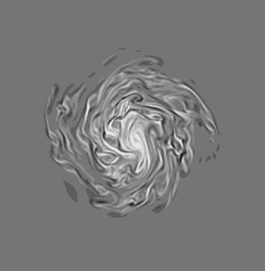
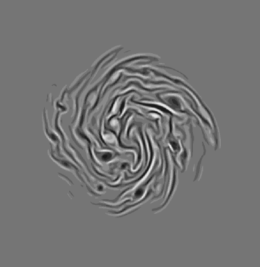
Figure 3: Vorticity (figure 3a) and current (figure 3b) at time $t=10$ for a magnetized, two–dimensional initially Keplerian disk with no initial background current.

Figures 1, 2 show the vorticity field for a simulation, in which the initial perturbation energy was normalized so that $\tilde{E}/E_{kep}\approx 0.005$. The vorticity is shown at the times $t=5$ (figure 1) and $t=10$ (figure 2). Figure 3 shows a section of the vorticity field at time $t=0$ (the initial condition) and at time $t=5$. The average vorticity profile remains Keplerian for the whole simulation and the rotation curves show bumps like those seen on rotation curves of galaxies.

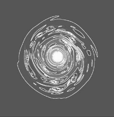
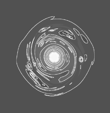
Figure 1: Section of the vorticity field of a perturbed two–dimensional Keplerian disk, at time $t=0$ and $t=5$.

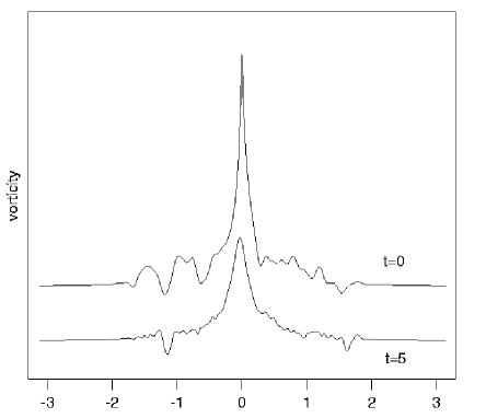
Figure 2: Section of the vorticity field of a perturbed two–dimensional Keplerian disk, at time $t=0$ and $t=5$.

These results show that long-lived, coherent anticyclonic vortices form in Keplerian shears, starting from an initially random perturbation field. Several other simulations, including ones with different energies in the Keplerian profile, different shapes of the initial perturbation, and different ratios between the energy of the perturbation and that of the unperturbed disk have given analogous results, provided that the perturbation energy $\tilde{E}$ was larger than a certain threshold. For the value of the hperviscosity $\nu_{2}=5\cdot 10^{-8}$ used in the previous simulation, the requirement is that $\tilde{E}/E_{kep}$ should be larger than about 0.001 for sustained vortices to form. The fate of nonlinear perturbations did not, as might have been supposed, lead to disorganized motions, but to coherent structures. These are anticyclonic vortices and they typically survive for tens or even hundreds of rotation times before being dissipated. Whether the final dissipation is a numerical artifact or a real phenomenon is not decidable as yet and this may be relevant to a discussion about whether the Keplerian profile should be considered as nonlinearly unstable or not (Balbus and Hawley 1996; Dubrulle and Zahn 1991). When we ran simulations with Newtonian viscosity, $p=1$, and $\nu_{1}=2\cdot 10^{-4}$ in eq.(14)), we found that coherent vortices form in this case as well. The only difference is that the vortices obtained with $p=1$ are slightly broader than those obtained with a $p=2$ hyperviscosity, as commonly observed for turbulence simulations in a homogeneous background flow.

The size of the viscosity coefficient plays an interesting role. The larger is the viscosity, the broader are the vortices. For large values of $\nu_{2}$, small vortices cannot form and only a few of the largest vortices survive. Conversely, the smaller is the viscosity, the more numerous the small-scale vortices are. Simulations with $\nu_{2}=5\cdot 10^{-9}$ show the presence of many small-scale anticyclonic vortices that penetrate well inside the central regions of the Keplerian disk. The smaller is the viscosity, the smaller is the minimum energy ratio $\tilde{E}/E_{kep}$ which is required in order to generate the vortices.

The roles of both the amplitude of the initial disturbance and of the viscosity emerge in the definition of two length scales that are used in discussions of geostrophic turbulence. In the present context, a length relating to the shear, $L_{S}=\sqrt{U/\Omega^{\prime}}$ may be defined where $\Omega^{\prime}=d\Omega/dr$ and $U$ is a characteristic initial velocity disturbance. The shear length, $L_{S}$ is the disk analogue of the Rhines scale of geostrophic turbulence theory (see Cho and Polvani 1996a; 1996b). In both situations, where the rotation rate varies in one direction, it is found that perturbations with scales greater than $L_{S}$ become highly anisotropic. It is believed that such structures do not participate in the inverse cascade of energy and remain elongated. Their decay takes place through radiation of Rossby waves.

Distinct vortices can form only with sizes less than $L_{S}$. On the other hand, vortices that are too small will be rapidly destroyed by viscosity. The viscous decay time of a structure of size $L$ is of the order of $L^{2p}/\nu_{p}$. For a vortex to live several rotation periods, this time must be much larger than $\Omega^{-1}$, which requires $L\gg L_{\nu}=(\nu_{p}/\Omega)^{1/2p}$. Thus, we expect that the copious formation of coherent vortices will be possible only if $L_{\nu}\ll L_{S}$. If the viscosity is too large, or the shear is too strong, $L_{\nu}$ and $L_{S}$ become comparable and vortices cannot form. For $p=1$ and with $\Omega/\Omega^{\prime}=r$, the criterion is that $Ur/\nu\gg 1$. Though this is in a sense to be expected, the ingredients in the derivation are somewhat different than they are in the usual derivation of criteria involving the Reynolds number. Our Reynolds number is the ratio of the $\beta$ term from the Coriolis force to the viscous term.

We have observed in these simulations that vortices form from general perturbations having initial sizes of the order of $L_{\nu}$. The vortices then merge with each other, and the size of the surviving vortices grows with time. In a homogeneous background, the only limit to this growth is set by the size of the domain. In a shear flow, the scale $L_{S}$ sets an upper limit to the vortex size. Thus, the older is a vortex, the closer its size is to $L_{S}$. At late evolutionary stages, most anticyclonic vortices have a size comparable with $L_{S}$. Since the strength of the local shear depends on the radius $r$, and $L_{S}=L_{S}(r)$, the range of radii in which vortices form will depend on the variation of $\nu$, hence density, with $r$. In the present simulations with constant $\nu_{p}$, we see larger vortices farther out.

4 Magnetic Effects

The inclusion of a magnetic field in the disk can produce linear instability and so change the fluid dynamics in an important way (Balbus and Hawley 1998). We study the effect of a purely horizontal magnetic field on the disk dynamics discussed in the previous section in the usual MHD approximation with displacement current neglected. The field is assumed to be not so strong as to modify the thin layer assumptions. We express it in terms of a scalar magnetic potential $a({\bf r},t)$ such that the horizontal field ${\bf B}=(B_{x},B_{y})$ is given by $B_{x}=-\partial a/\partial y$ and $B_{y}=\partial a/\partial x$. This magnetic field is horizontally non-divergent so any vertical field that is present must be independent of $z$.

The current is $\nabla\times{\bf B}$ and is in the vertical direction. This does not fit in well with the thin layer image and is more suited to the picture of two-dimensional incompressible flow. We nevertheless proceed formally to consider what happens when the Lorentz force ${\bf j}\times{\bf B}$ is included in the dynamics of the previous section, where the current ${\bf j}$ is purely in the $z$-direction and its magnitude is given by

$$j=\nabla^{2}a\ .$$ (17)

The equation of motion for the vertical vorticity becomes

$${{\partial\zeta}\over{\partial t}}+[\psi,\zeta]-[a,j]=D_{\zeta}$$ (18)

where the various quantities are as before. In addition, the induction equation for the magnetic field, when expressed in terms of the magnetic potential, is

$${{\partial a}\over{\partial t}}+[\psi,a]=D_{a}\ .$$ (19)

The Ohmic dissipation $D_{a}$ term is given by

$$D_{a}=(-1)^{q-1}\eta_{q}\nabla^{2q}a\ .$$ (20)

In the absence of dissipation, eqs.(18) and (19) have three quadratic invariants: the total (kinetic plus magnetic) energy $E=1/2\int(\nabla\psi)^{2}dxdy+1/2\int(\nabla a)^{2}dxdy$, the integral of the squared magnetic potential, $A=\int a^{2}dxdy$, and the cross helicity $H=\int{\bf u}\cdot{\bf B}dxdy$. The simultaneous conservation of these quantities induces a direct cascade of energy, from large to small scales, and an inverse cascade of magnetic potential, from small to large scales (Fyfe & Montgomery 1976; Fyfe et al. 1977). One thus expects to see coherent structures in the current field rather than in the vorticity. Since the three-dimensional MHD equations have three quadratic invariants as well, the fact that energy cascades to small scales, makes 2D MHD closer to the full three-dimensional MHD problem than 2D Navier-Stokes is to 3D hydrodynamics.

The 2D MHD system has a wide range of dynamical behaviours. In the limit of weak magnetic field, the magnetic potential behaves as a passive scalar, and the term $[a,j]$ in eq.(18) can be discarded. In this limit, one recovers the behavior of the 2D Navier-Stokes equations (13). An initially weak magnetic field does however grow with time, and in later stages the dynamics is significantly affected by magnetic forces.

An important diagnostic quantity is the global correlation between the velocity and the magnetic fields defined as $C=H/E$. If the velocity and magnetic fields are nearly aligned, the absolute value of the global correlation coefficient is close to one. Several simulations have shown that, if $|C|$ is larger than about 0.2 initially, then it grows with time toward the value $|C|=1$. In this process, called dynamic alignment, Lorentz forces cause the magnetic and velocity fields to become parallel (or anti-parallel) to each other. On the other hand, if $C\approx 0$ initially, then the two fields remain uncorrelated.

Numerical simulations of the dissipative 2D MHD equations with $D_{\zeta}\neq 0$ and $D_{a}\neq 0$, in a homogeneous background reveal the formation of current and vorticity sheets (Biskamp & Welter 1989). Coherent magnetic vortices also form and dominate the current distribution and the dynamics of the system (Kinney et al. 1995) so that, at later times, the fluid vorticity plays a minor role, concentrating in sheets at the periphery of the magnetic vortices. In the individual magnetic vortices, there may be a non-zero correlation between vorticity and current. The sign of this correlation is different in different vortices, leading to an approximately zero global correlation between the magnetic and the velocity fields.

The question that we consider here is whether magnetic vortices can form in a shearing background. To address this issue, we have run a series of simulations on the behavior of a magnetized, barotropic Keplerian disk, by modifying the code described in the previous section to deal with (18)-(19). In the runs discussed below, we have chosen a hyperviscous dissipation with $p=q=2$, $\nu_{2}=5\cdot 10^{-8}$ and $\eta_{2}=2.5\cdot 10^{-7}$. This gives a magnetic Prandtl number $Pr_{mag}=\nu_{2}/\eta_{2}=0.2$. Runs with $Pr_{mag}=1$ have provided analogous results.

In simulating a magnetized disk, we have to specify the initial background current distribution. Though it seems likely that an initial field will quickly develop a strong toroidal presence, we have decided to leave the matter open, and so we show the results of two different simulations. In the first, we assume no background current; here the magnetic field is present only as a perturbation of a basically unmagnetized background state. In the second type of simulation, we assume the presence of a Keplerian background current, with the same amplitude as the background vorticity field at the outset. In both cases, the background vorticity is assumed to be Keplerian, as in Section 3.

In the case with no background current, the background Keplerian vorticity field has energy $E_{kep}=0.5$. The typical rotation time at $r=\pi/4$ is $T_{kep}(\pi/4)\approx 2$ and the simulation has been run up to a time $T=20$. In this simulation, we initially perturb the magnetic field away from zero and do not perturb the vorticity; the perturbation energy is $\tilde{E}\approx 0.004E_{kep}$. The spectrum of the initial magnetic perturbation is given by eq.(16). This case is characterized by an almost zero correlation between the initial magnetic and velocity fields.

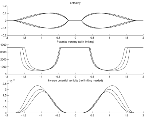
Figure 5: Enthalpy (top), potential vorticity (middle), and potential thickness (bottom) for three thin disks having respectively $n_{o}={3/4}$, ${4/4}$ and ${5/4}$.

Figures 4 and 5 show the vorticity and the current at time $t=10$ and they reveal that strong magnetic vortices form in the presence of an initial Keplerian shear. As already observed by previous studies without a background shear, the vorticity is dominated by magnetic effects, with fluid vorticity concentrating in sheets and in weaker structures associated with the magnetic vortices. In the evolved fields, there is no global correlation between vorticity and current.

A significant difference from the non-magnetic case is found in the evolution of the mean vorticity profile. Without the magnetic field the Keplerian profile is linearly stable to perturbations and we find that the average radial profile remains Keplerian during the evolution. In the MHD simulation shown here, the presence of the magnetic perturbation leads to a modification of the background Keplerian profile, which becomes flatter as the evolution proceeds. This is not surprising, as the magnetic torques enter the dynamics significantly.

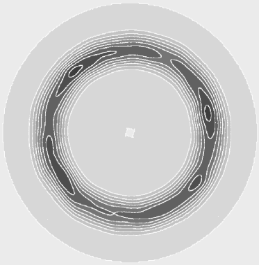
Figure 6: Potential thickness (inverse potential vorticity) at time $t=2$ for a perturbed thin disk with $n_{i}=3/4$ and $n_{o}=5/4$.

Figures 6 and 7 show the vorticity and the current obtained when the current has a background Keplerian component $J(r)$, equal in strength to the background vorticity profile $\Omega(r)$. No vortices form in this case, the two fields becoming rapidly fully correlated and frozen into alignment due to the presence of an initial correlation $|C|>0.2$. The terms $[\psi,\zeta]$ and $[a,j]$ then cancel each other in eq.(18), and the field remains in its Keplerian state, slowly decaying due to dissipation.

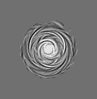
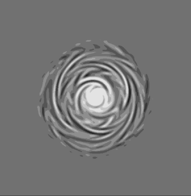
Figure 4: Vorticity (figure 4a) and current (figure 4b) at time $t=10$ for a magnetized, two–dimensional initially Keplerian disk with an initially Keplerian background current.

These simulations have thus shown that, when there is no background Keplerian current, coherent magnetic vortices can be generated. In the magnetic field, the strong cyclone-anticyclone asymmetry observed for purely hydrodynamic disks is absent. The vorticity field is dominated by the magnetic effects, and weaker vorticity concentrations can be observed in the magnetic vortices. In the absence of a background Keplerian current, the vorticity profile does not remain Keplerian. These results are restricted to the unrealistic case of purely horizontal magnetic field and do not include the influence of an external gravitational force that might favor the maintenance of the Keplerian background flow. In the appendix we describe the inclusion of this effect and observe that it does not change the general character of the results.

5 Disks With Variable Surface Density

The full thin-layer theory is like that of a two-dimensional compressible fluid, where density fluctuations are important, except that in the thin-layer approximation these fluctuations propagate as compressible gravity waves rather than acoustic waves (Qian & Spiegel 1994). We present here some first results from numerical simulations of the full thin-layer problem. This problem is computationally more demanding than the version we have just considered so that they involve even more modest parameter values than the incompressible case. We begin by recalling some of the theoretical background for the thin-layer simulations (Balmforth et al. 1992). To do that, we temporarily ignore the viscous term in order to keep the discussion simple; it is restored for the numerical computations.

In the full thin-layer theory of section 2, we solve the continuity equation (8) together with the vertically integrated counterpart of the momentum equation (1). Since vertical motions are negligible in thin layers, we have hydrostatic balance in the vertical direction. The simplified ${\hat{z}}$-component of the momentum equation then integrates to:

$$\int_{-h}^{h}{1\over\rho}{\partial p\over\partial z}dz=\int_{-h}^{h}{\partial H\over\partial z}dz=-\int_{-h}^{h}{\partial\Phi\over\partial z}dz,$$ (21)

where we have introduced the specific enthalpy $H$ according to the definition provided by the first equality in (21). For a thin layer, the thickness of the disk, from $h$ above to $-h$ below the plane, is small compared to the radial coordinate, $r$, so this equation tells us that the enthalpy is well approximated by

$$H={GM\over 2r^{3}}\left(h^{2}-z^{2}\right)\ .$$ (22)

Since the pressure, and therefore the enthalpy, vanishes at $z=\pm h$, (21) and (22) become

$$\eta(x,y,t)=H(x,y,0,t)={GMh^{2}\over 2r^{3}},$$ (23)

where $\eta$ is the specific enthalpy to be used in the thin layer. Then, an effective equation of state for the layer can be found by substituting the polytropic formula for enthalpy, $H=K{\gamma\over\gamma-1}\rho^{\gamma-1}$, into (21), allowing the density to be expressed as a function of the disk thickness; we get

$$\rho=\left[{\gamma-1\over\gamma K}{GM\over 2r^{3}}\left(h^{2}-z^{2}\right)\right]^{1/\gamma-1}.$$ (24)

This relation, when inserted into the definition of the surface density, equation (7), yields the vertically integrated equation of state,

$$\sigma=\sigma_{0}\left[\eta^{\gamma+1\over\gamma-1}r^{3}\right]^{1/2},$$ (25)

where $\sigma_{0}$ is a constant. Because of the dependence on the local vertical gravity, the equation of state depends on $r$.

The horizontal momentum equation is now

$${{D{\bf u}}\over{Dt}}=-\nabla\left(\eta+\phi\right)+{\bf D}_{\bf u}$$ (26)

where $u$ is the two-dimensional velocity ${\bf u}=(u,v)$, $\phi$ is the gravitational potential in the plane ($\phi(x,y)=\Phi(x,y,0)$) and the viscous term has been restored. The expression for the potential vorticity of the disk has been given in equation (10).

We have solved equations (8), (25) and (26) in finite-difference form, on grids of $256\times 256$ and $512\times 512$ using a modified form of the Miami Isopycnal Coordinate Model (MICOM), a second order algorithm which incorporates a flux-corrected transport of the surface density. This code has been used successfully for a wide variety of oceanic flows; in particular, it has been used to study the ocean thermocline, another thin layer whose equations are like the ones studied here. The special feature of this code, not contained in typical shallow fluid codes, is that it allows for a vanishing layer thickness (Sun et al. 1993).

For the initial conditions, we need a background disk. For this we used steady axisymmetric models with angular velocity profile given by

$$\Omega=\left({1\over r}{d{\bar{\eta}}\over dr}+{1\over r}{d\phi\over dr}\right)^{1/2}\;,$$ (27)

where $\bar{\eta}$ is the time-independent enthalpy. When (as is usual in the mean state) the enthalpy variations are negligible, we recover from (27) the Keplerian velocity $\Omega_{K}=r^{-3/2}$ for the potential $\phi=-1/r$.

Since enthalpy variations are not negligible, the variations of the background surface density lead to both a departure from Keplerian flow, according to (27), and to a modulation of the background potential vorticity, according to (10) in a way that is analogous to topographic effects frequently encountered in geophysical problems.

To simplify the application of boundary conditions, we have taken the case of an annulus with enthalpy distribution

$$\bar{\eta}(r)=\eta_{0}(r-r_{i})^{n_{i}}(r_{o}-r)^{n_{o}},$$ (28)

where the subscripts $i$ and $o$ mean inner and outer. This $\bar{\eta}$ vanishes at two radii ($r=r_{i}$ and $r=r_{o}$), always chosen to be well within the computational domain. Since we apply boundary conditions only on the edges of the domain, this makes for an insensitivity to the boundary conditions.

The computational domain extends from $-2$ to $2$ and we have used typical values for the inner and outer disk radii of $1/4$ and $7/4$, respectively. The computations were performed in a frame co-rotating with the radius $r=1$. The angular velocities do not depart significantly from Keplerian values; at $r=1/3$ the orbital period is $\approx 1$.

In figure 8 we display the enthalpy for three steady disks, having $n_{i}={3\over 4}$ and $n_{o}={3\over 4},{4\over 4},{5\over 4}$. The corresponding potential vorticity is also plotted (middle), but since $q$ is not well defined where $\sigma$ vanishes, we plot only those regions where the surface density exceeds some minimum value: $\sigma>\sigma_{0}$. The singular nature of $q$ indicates the presence of a boundary layer at the disk edges. At present we are interested only in the behavior far from such boundary layers, so we can choose to represent the inverse of $q$, or what is called the potential thickness (figure 8, bottom), rather than the potential vorticity.

In shallow fluids, gravitational forces will act to restore perturbations made to the layer thickness. But in the presence of rotation, this process excites local shears in the flow. Large perturbations will be deformed in this process since there is a scale above which rotation dominates vertical stability. In geophysics this critical scale is called the (Rossby) deformation radius, $L_{D}$ (Pedlosky 1987), given by $L_{D}^{2}=2\bar{\eta}r/f^{2}h$. Vortices larger than the Rossby radius have quiet centers encircled by rings of rapidly varying potential vorticity. This manifestation of $L_{D}$ has been revealed by numerous laboratory and computational results, which show how $L_{D}$ constrains the extent of the perturbing shear layers within a vortex.

To study the action of potential vorticity and the behavior of potential vortices in disks, we perturb the steady solutions given above. One way to introduce small disturbances of $q$ is to simply perturb the thickness. To leading order, the perturbed potential vorticity can be expressed as

$${q}=\bar{q}-{\sigma^{\prime}\over\bar{\sigma}}\bar{q}+{\zeta^{\prime}\over\bar{\sigma}},$$ (29)

where the last term is absent if we do not perturb the absolute vorticity. Using this expression, we build a random distribution of perturbed potential vorticity, whose energy peaks at a wavelength $\lambda\sim R_{disk}/10$, and superpose this onto the steady disk.

The evolution of the initial disk given by (27) and (28) leads to an approximately steady disk with some negligible migration of surface density toward $r=0$ as a result of viscous stress. When the initial condition includes a perturbed potential vorticity as described above and in (29), the evolution is dominated by the interaction of compressible vortices with each other and with the background shear. The disk at time $t=2$ is shown in figure 9.

The most obvious features found in the potential vorticity are: (1) vortices which are too small are quickly eliminated by the combined actions of the shear and dissipation; (2) small potential vortices, if they are above this scale, rapidly coalesce to form larger, more coherent features; (3) cyclonic fluctuations tend to be easily absorbed into the background shear of the disk; (4) the more robust anticyclones can persist for many disk rotations.

6 Conclusions

At first sight it might seem that strong shears provide an abundant source of angular momentum that would feed vortex production and that would tightly wind local magnetic anomalies. However, shears also work against the conventional vortex formation process by making the environment highly anisotropic. In the context of the Jovian atmosphere, shears also occur and the work on that situation suggests that vortices cannot form if they are too large (Cho and Polvani 1996a; 1996b). Instead, large structures give rise to bands in the jovian atmosphere. We may expect a similar behavior in disks and some of our shallow water calculations have revealed large scale vortical structures with banded, spiral character (Yecko 1995). However, the calculations reported here show that when the local disturbances are not so large, vortices form in disks and that similar coherent structures form in mildly magnetized disks.

In order to form these coherent structures, we need to have initial perturbations of finite amplitude. There is no doubt that these are available in magnetized disks since they are linearly unstable. The case of nonmagnetized disks is apparently in dispute. The systems we have studied are not unstable within the numerical schemes we have been using. Rather, they are excitable. This means that a finite amplitude disturbance with amplitude above a given threshold goes through an interesting evolution (in fact formation of vortices) before the system returns to its initial Keplerian state. If there were no magnetic fields, we would need to provide a source of perturbations to produce vortices. These could be present even in nonturbulent disks around black holes since they may be buffeted continually by incoming objects. On the other hand, magnetized disks will certainly have a continual source of perturbations.

In any case, our numerical simulations of two-dimensional, barotropic disks and of thin-layer, compressible disks have shown that sufficiently energetic vorticity perturbations evolve into long-lived, coherent vortices that may heavily affect the disk dynamics in several ways before they decay. In the presence of magnetic effects, coherent magnetic vortices are formed instead of purely kinetic vorticity structures. These will likely give rise to a good deal of variability and other phenomena seen on stars with similar activity.

Appendix A Forcing Keplerian Flows

In the previous sections we have discussed the evolution of a free Keplerian disk, i.e., of a freely-decaying, initially perturbed Keplerian profile. In the pure hydrodynamic case, the average profile remains Keplerian, except for the fact that it is slowly dissipated by the small hyperviscosity. In the MHD case, the average vorticity profile rapidly becomes non-Keplerian.

On the other hand, we may suppose that external forces, which are not described by the simple evolution equations used above, try to mantain a background Keplerian rotation. These could be, for example, the gravity of the central mass and the slow infall of material at the edge of the disk. In this section, we study the evolution of a perturbation of a Keplerian disk, whose average profile is forced to remain Keplerian.

Suppose that the vorticity field is the sum of two terms, a constant Keplerian background $\Omega(r)$, imposed from the outside, and a perturbation $\tilde{\zeta}({\bf r},t)$ which is free to evolve. Dissipation is assumed to act only on the perturbation field $\tilde{\zeta}$. For a purely hydrodynamic disk, the equations of motion become in this case

$${{\partial\tilde{\zeta}}\over{\partial t}}+[\tilde{\psi},\tilde{\zeta}]=\tilde{D}_{\zeta}\ -[\Psi,\tilde{\zeta}]-[\tilde{\psi},\Omega]$$ (30)

where $\Omega(r)$ is the constant Keplerian profile, $\Psi(r)$ is the corresponding stream-function, $\tilde{\zeta}$ and $\tilde{\psi}$ are the vorticity perturbation and perturbation stream-function, and $\tilde{D}_{\zeta}=(-1)^{p-1}\nu_{p}\nabla^{2p}\tilde{\zeta}$ is the dissipation. The Keplerian profile is a solution to the equation $[\Psi,\Omega]=0$, this term is thus absent from eq.(30).

The term $F=-[\Psi,\tilde{\zeta}]-[\tilde{\psi},\Omega]$ represents an external forcing on the evolution of the perturbation. If the perturbation were capable of extracting energy from the overall rotation of the disk, then it could grow and eventually stabilize, without being necessarily dissipated. From another point of view, this approach allows for studying the stability of a Keplerian disk, by following the evolution of an initial perturbation. This is just a special case of the general study of the stability of (barotropic) shear flows. Numerical simulation of eq.(30) has shown that anticyclonic vortices form in this case as well, notwithstanding the continuous forcing. The perturbation does, however, decay with time and simulations run with other values of the disk parameters — viscosity, ratio of the perturbation energy to the energy of the background Keplerian flow, etc. — have led to analogous results.

In the MHD case, the magnetic field acts as a catalyst that allows the vorticity perturbation to extract energy from the Keplerian shear. For a forced MHD disk the equations are

$${{\partial\tilde{\zeta}}\over{\partial t}}+[\tilde{\psi},\tilde{\zeta}]-[\tilde{a},\tilde{j}]=\tilde{D}_{\zeta}-[\Psi,\tilde{\zeta}]-[\tilde{\psi},\Omega]$$ (31)

$${{\partial\tilde{a}}\over{\partial t}}+[\tilde{\psi},a]=\tilde{D}_{j}$$ (32)

where $\tilde{a}$ and $\tilde{j}=\nabla^{2}\tilde{a}$ are the perturbation on the magnetic potential and the current and $\tilde{D}_{j}=(-1)^{q-1}\eta_{q}\nabla^{2q}j$. We have supposed no background Keplerian current and the forcing is acting only in the vorticity equation.

The numerical simulation of eqs.(31,32) has shown that magnetic vortices do form also in the presence of a continuous forcing. In this case, however, the perturbation energy grows with time, and the Keplerian MHD disk is unstable. The presence of the magnetic fields acts as a trigger for the instability, and the kinetic energy of the perturbation grows with time. Notwithstanding the Keplerian forcing on vorticity, also in this case the background vorticity profile does not remain Keplerian.

References

- [Abramowicz et al. (1991)] Abramowicz, M. A., Lanza, A., Spiegel, E. A. & Szuszkiewicz, E. 1991 Nature 356, 41–43.
- [Babiano et al. (1994)] Babiano, A., Boffetta, G., Provenzale, A. & Vulpiani, A. 1994 Phys. Fluids 6, 2465–2474.
- [Balbus & Hawley (1996)] Balbus, S. A. & Hawley, J. F. 1996 Astrophys. J. 467, 76–86.
- [Balbus & Hawley (1998)] Balbus, S. A. & Hawley, J. F. 1998 Rev. Mod. Phys. , in press.
- [Balmforth et al. (1992)] Balmforth, N. J., Meacham, S. P., Spiegel, E. A. & Young, W. R. 1992 Ann. N.Y. Acad. Sci. 675, 53–64.
- [Benston & Lighthill (1982)] Bengston, L. & Lighthill, J., Eds. 1982 Intense Atmospheric Vortices, Springer-Verlag.
- [Biskamp & Welter (1989)] Biskamp, D. & Welter H. 1989 Phys. Fluids B 1, 1964–1979.
- [Charney (1971)] Charney, J. G. 1971 J. Atmos. Sci. 28, 1087–1094.
- [Cho & Polvani (1996a)] Cho, J. Y.-K. & Polvani, L. M. 1996a Science 273, 335–337.
- [Cho & Polvani (1996b)] Cho, J. Y.-K. & Polvani, L. M. 1996b Phys. Fluids 8, 1531–1552.
- [Dowling & Spiegel (1990)] Dowling, T. E. & Spiegel, E. A. 1990 Ann. N.Y. Acad. Sci. 617, 190–216.
- [Dubrulle & Zahn (1991)] Dubrulle, B. & Zahn, J.-P. 1991 J. Fluid Mech. 231, 561–573.
- [Elhmaidi et al. (1993)] Elhmaidi, D., Provenzale, A. & Babiano, A. 1993 J. Fluid Mech. 257, 533–558.
- [Fyfe & Montgomery (1976)] Fyfe, D. & Montgomery, D. 1976 J. Plasma Phys. 16, 181.
- [Fyfe et al (1977)] Fyfe, D., Joyce, G. & Montgomery, D. 1977 J. Plasma Phys. 17, 317.
- [Ghil & Childress (1987)] Ghil, M. & Childress, S. 1987 Topics in Geophysical Fluid Dynamics Springer-Verlag.
- [Hopfinger et al. (1982)] Hopfinger, E. J., Browand, F. K. & Gagne, Y. 1982 J. Fluid Mech. 125, 505–534.
- [Hunter & Horak (1983)] Hunter, J. H. & Horak, T. 1983 Astrophys. J. 265, 402-416.
- [Kinney et al (1995)] Kinney, R., McWilliams, J. C. & Tajima, T. 1995 Phys. Plasmas 2, 3623–3639.
- [Kraichnan & Montgomery (1980)] Kraichnan, R. H. & Montgomery, D. 1980 Reports Progr. Phys. 43, 547–619.
- [Llewellyin Smith (1996)] Llewellyin Smith, S. G. 1996 Vortices and Rossby-wave radiation on the beta-plane , Thesis, DAMTP, Cambridge University.
- [McWilliams (1984)] Mc Williams, J. C. 1984 J. Fluid Mech. 146, 21–43.
- [McWilliams (1990)] Mc Williams, J. C. 1990 J. Fluid Mech. 219, 361–385.
- [Nezlin & Snezhkin (1993)] Nezlin, M. V. & Snezhkin, E. N. 1991 Rossby Vortices, Spiral Structure and Solitons, Springer-Verlag.
- [Pedlosky (1987)] Pedlosky, J. 1987 Geophysical Fluid Dynamics, Springer-Verlag.
- [Provenzale et al. (1997)] Provenzale, A., Babiano, A. & Zanella, A. 1997 in Mixing: Chaos and Turbulence, NATO–ASI, Cargese, France; Plenum, in press.
- [Qian et al. (1991)] Qian, Z. S., Spiegel, E. A. & Proctor, M. R. E. 1991 Stab. App. An. Cont. Med. 1, 73–93.
- [Qian & Spiegel (1994)] Qian, Z. S. & Spiegel, E. A. 1994 Geophys. Astr. Fluid Dyn. 74, 225–243.
- [Rhines (1979)] Rhines, P. B. 1979 Ann. Rev. Fluid Mech. 11, 401–411.
- [Sun et al. (1993)] Sun, S., Bleck, R. & Chassignet, E.P. J. Phys. Ocean. 23, 1877–1884.
- [Tanga et al. (1996)] Tanga, P., Babiano, A., Dubrulle, B. & Provenzale, A. ICARUS 121, 158–170.
- [Yecko (1995)] Yecko, P. A. 1995 Ann. N.Y. Acad. Sci. 773, 95–110.