Abstract

Experimental results from Haverah Park, Yakutsk, AGASA and Fly’s Eye are reviewed. All these experiments work in the energy range above $10^{17}$ eV. The ’dip’ structure around $10^{18.5}$ eV in the energy spectrum is well established by all the experiments, though the exact position differs slightly. Fly’s Eye and Yakutsk results on the chemical composition indicate that the cosmic rays are getting lighter over the energy range from $10^{17}$ eV to $10^{19}$ eV, but the exact fraction is hadronic interaction model dependent, as indicated by the AGASA analysis. The arrival directions of cosmic rays are largely isotropic, but interesting features may be starting to emerge. Most of the experimental results can best be explained with the scenario that an extragalactic component gradually takes over a galactic population as energy increases and cosmic rays at the highest energies are dominated by particles coming from extragalactic space. However, identification of the extragalactic sources has not yet been successful because of limited statistics and the resolution of the data.

subject headings: cosmic rays: general

1 Introduction

Many kinds of radiation exist in the universe, including photons and particles with a wide range of energies. Some of the radiation is produced in stars and galaxies, while some is cosmological background radiation, a relic from the history of cosmic evolution. Among all this radiation, the most energetic are cosmic ray particles: nucleons, nuclei, and even extremely energetic gamma rays. Their energies appear to reach beyond $10^{20}$ eV. Cosmic rays with energies above $10^{19}$ eV were first detected by the Volcano Ranch group led by John Linsley of the University of New Mexico more than 30 years ago. Since then, where and how these particles are produced and how they propagate in space have been puzzles. Their extremely high energies, seven orders of magnitude greater than those of any nucleons that humans have thus far been able to accelerate on earth, suggest that unbelievably energetic phenomena have occurred somewhere in the universe. One problem is that the extremely low flux at these energies (the typical rate of cosmic rays above $10^{20}$ eV is one event/km²/century!) requires a detector with a huge acceptance which has always been challenging to build due to technological and economical difficulties. The pioneer detector at Volcano Ranch covered an area of only 9 $km^{2}$. Experiments following Volcano Ranch have improved in terms both of statistics and data quality. Throughout these years of continuous effort, signatures concerning the origin of these Extremely High Energy Cosmic Rays (EHECRs) have started to emerge.

In this paper we review the current situation of our understanding of the origin of EHECRs, based mainly on recent observational results. To help our interpretation of the data, we first discuss the conditions required for a site to be a source of EHECRs, and briefly describe how these cosmic rays propagate through space. Next the techniques of detecting these particles are summarized and the major detectors are introduced. Following that, the recent experimental results are reviewed in terms of the energy spectrum, chemical composition, and anisotropy. A two component model, which we think is highly reasonable, is constantly checked against these results. Finally, the consistency of the results compared with the simple model is summarized.

1.1 Extremely High Energy Cosmic Rays: General View

Figure 1: A schematic drawing of the energy spectrum of cosmic rays above $10^{14}$ eV.

The energy spectrum of high energy cosmic rays above 10 GeV (where the magnetic field of the sun is no longer a concern) is well represented by a power law form. Figure 1 is a schematic drawing of the energy spectrum. In terms of its structure, the spectrum can be divided into three regions: two “knees” and one “ankle”. The first “knee” appears around $3\times 10^{15}$ eV where the spectral power law index changes from -2.7 to -3.0. The second “knee” is somewhere between $10^{17}$ eV and $10^{18}$ eV where the spectral slope steepens from -3.0 to around -3.3. The “ankle” is seen in the region of $3\times 10^{18}$ eV. Above that energy, the spectral slope flattens out to about -2.7, however, there is large uncertainty due to poor statistics and resolution. Our interest in this paper is this final and most energetic population, the EHECRs. The production of the first two populations is likely to be explained with conventional first order Fermi shock acceleration [1] at energetic objects such as supernova remnants within our galaxy, although many concerns about the effectiveness remain. The third population is interesting since it raises the following difficult questions: How do they get such huge energies? Where do they come from? Does the spectrum end somewhere? What is the chemical composition of these cosmic rays?

1.2 The Possible Sites to Produce EHECRs

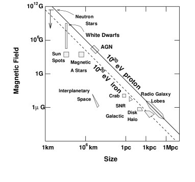
Figure 2: The Hillas Diagram showing possible sites for acceleration of cosmic rays up to $10^{20}$ eV.

The existence of cosmic rays with energies up to nearly $10^{20}$eV has been solidly established, but the acceleration theories are on much less solid footing. No matter how the particles are accelerated, the upper bound of the energy gained should be determined by balancing the acceleration time with escape time from the acceleration site. In 1984, Hillas proposed the following constraint [2]:

$$B_{\mu G}L_{pc}>{E\over 10^{15}\ eV}{1\over Z\beta},$$

where $L_{pc}$ is the size of the site in parsec, $Z$ is charge of the particle, and $\beta$ is the speed of the scattering waves within the field of the site. The magnetic field needs to be large enough to confine the particles within their acceleration site and the size of the site must be sufficiently large for particles to gain sufficient energy before they escape. These simple requirements already rule out most astronomical objects in the universe. Figure 2 shows objects which satisfy this dimensional requirement. Most of the galactic objects are excluded simply because they are too small and/or have magnetic fields that are too weak. Only a few extragalactic objects such as Active Galactic Nuclei (AGN) and radio galaxies remain as possible candidates. This fact is the basic reason many favor the extragalactic origin of EHECRs.

In any actual acceleration site, energy loss mechanisms always compete with the gain of energy. With first order Fermi shock acceleration, the acceleration time is proportional to the mean free path for scattering in the shock wave, which itself is approximately inversely proportional to the magnetic field strength. Therefore, a certain magnitude of magnetic field is required, not only to confine the particles within the site, but also to accelerate the particles quickly. However, too strong a magnetic field also causes problems for particle acceleration, because it can cause protons to lose energy via synchrotron radiation. Other strong energy losses are caused by collisions with photons and/or matter at the acceleration site. A certain photon field is normally expected at the site as a result of synchrotron radiation by electrons or thermal radiation off the accretion disk. This leads to the additional requirement, that the site must have sufficiently low densities of radiation and matter so that cosmic ray nucleons are able to accelerate to $\sim 10^{20}$ eV before losing significant energy. This raises more difficulties with candidate sites. For example, the core region of AGNs are ruled out because for this reason. The relativistic jets found in some classes of AGNs such as blazars may be able to produce EHECRs [3, 4], although models require optimistic fine-tuning of the acceleration efficiency and the Doppler boost factor of the relativistic jets. Rachen and Biermann have proposed hot spots of Fanaroff-Riley type II galaxies as EHECR sources [5]. There seems to be enough acceleration power with not too-dense photons at the hot spots. However, the possibility is not excluded that collisions with UV photons in the spots discourage the acceleration of protons above $10^{20}$ eV. While relativistic jets of blazars and hot spots of FR II type radio galaxies are candidates sources of EHECRs via a conventional first order Fermi shock acceleration mechanism, it is not obvious that the acceleration efficiency is large enough to produce particles up to $10^{20}$ eV.

These extragalactic models favor protons for the EHECR composition. Heavier nuclei like iron may break up into nucleons by photodisintegration during the shock acceleration, through collisions with UV photons at the site.

The difficulties in acceleration can be avoided if EHECRs are direct products of processes which do not require acceleration. “Top down” scenarios have recently been proposed [6, 7] involving relics of symmetry-breaking phase transitions in the early universe such as cosmic strings and magnetic monopoles, so called topological defects. If such defects exist, they may have produced EHE particles with energies up to the grand unified theory (GUT) scale (typically $\sim 10^{25}$ eV) through the decay of the X-particles released in the collapse or decay of the defects. Because the hadron jets created at the decay of the X-particle are the main channels of particle production in this model, neutrinos and gamma rays, rather than protons and neutrons, are predominant. Any heavy nuclei like iron are completely ruled out in this model because the hadron jets create no nuclei. Propagation effects in the cosmic background radiation field (described later) would modify the emitting spectrum of each component, but one would still expect that gamma rays may be dominant at energies above $10^{20}$ eV, with details dependent on the strengths of the universal radio background and the extragalactic magnetic field, both of which are poorly known. The basic problem in this scenario, is that topological defects are exotic: the absolute intensity of defects is unknown. The observed intensities of cosmic rays and diffuse gamma rays can put constraints on the upper bound of defect intensity. So far, we have no experimental evidence, however, measurement of an excess of $\gamma$ ray flux above $10^{20}$ eV and detection of EHE neutrinos above $10^{19}$ eV would be signatures of topological defects.

It has been suggested that Gamma Ray Bursts (GRB), responsible for gamma rays up to the GeV range, may also be able to produce EHECRs. This would be a burst source and not a continuously emitting one. This would also result in a correlation between arrival times and energies of EHECRs. Unfortunately, the time scale might be much longer than any single experiment can afford to run and thus the correlation may be extremely difficult to detect. Detail on this idea is presented in [8, 9].

1.3 Propagation of EHECRs in space

It is important to understand how EHECRs propagate from their sources to earth, since this puts constraints on possible sources and provides hints for the most effective way of searching for them. First, the galactic magnetic field of $\sim\mu$G can no longer confine cosmic ray protons with energies greater than $10^{19}$ eV in the galactic disk since the Larmor radius of a proton at that energy,

$$L_{kpc}\simeq({E\over 10^{19}\ eV})({B\over 3\ \mu G})^{-1}\times 3kpc,$$

becomes greater than the thickness of our galactic disk. This means that any galactic protons can easily escape from our galaxy, provided that the galactic magnetic fields do not extend out into a possible Halo. This again favors the hypothesis of an energetic extragalactic component dominating galactic components in the EHECRs population.

Secondly, when EHECRs are traveling through extragalactic space, their trajectories are not strongly bent by the extragalactic magnetic field and the arrival directions of such cosmic rays should point back to their emitters. Information on the extragalactic magnetic field strength is difficult to gather. We know only the Faraday rotation bound on the extragalactic magnetic field is given by [10]

$$B_{rms}\sqrt{l_{c}}\leq 10^{-9}G\ Mpc^{1\over 2}$$

where $l_{c}$ is the scale of the coherent magnetic field in Mpc, and the mean deflection angle can be written as

$$\theta_{def}\leq({R\over 10Mpc})^{1\over 2}({E\over 3\times 10^{19}\ eV})^{-1}\times 3.2^{\circ}$$

for protons [11]. Here $R$ is distance to the source. This opens a new window of astronomy, that of Charged Particle Astronomy.

A typical deflection angle of $\sim 3^{\circ}$, which is comparable with the typical angular resolution of the present experiments, might be still too large in an actual search for sources, because there exist many astronomical objects in a $3^{\circ}\times 3^{\circ}$ window even if the candidates are limited to AGNs and radio galaxies. The real situation is much better, however, since there is a limit on the distance over which an EHECR may travel. We can limit the search to relatively nearby sources, because EHECRs collide with cosmological backgrounds and lose energy during their propagation. This is the most important effect on the propagation of EHECRs.

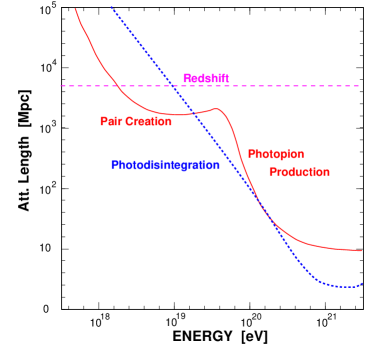
Figure 3: The attenuation length of cosmic rays as a function of energy. The solid curve shows the case for nucleons calculated by Yoshida and Teshima. The dashed curve shows the case for iron calculated by Puget, Stecker and Bredekamp. The bound given by redshift (adiabatic energy loss) are applicable to all primaries.

Figure 4: The expected spectral shapes for two assumptions concerning the distribution of sources in extragalactic space. $m$ is the evolution parameter of EHECR emission. A larger $m$ means more contributions from sources in distant (high redshift) regions. This extragalactic population might dominate in the highest energy region of the observed spectrum above $\sim 10^{19}$ eV. The galactic magnetic field, which could suppress the the recovery below $10^{18.5}$ eV, is not included in the simulation.

EHECR protons or neutrons interact with the microwave background photons through pair creation and photopion production. The threshold energy of photopion production, the main energy loss process, is

$$E\simeq 7\times 10^{19}({E_{bb}\over 2\times 10^{-3}\ eV})^{-1}(1+\cos\theta)^{-1}\quad eV$$

where $E_{bb}$ is the energy of the microwave background photon, from a blackbody spectrum with a characteristic temperature of $2.7^{\circ}$ K. The photon and the EHECR interact with a collision angle $\theta$. Above the threshold energy, EHECRs rapidly lose energy. This may result in a cutoff in the energy spectrum. This cutoff is known as Greisen-Zatsepin-Kuzmin cutoff (GZK cutoff) [12, 13], and is the centerpiece of the EHECRs physics. A detection of this effect proves the extragalactic origin of EHECRs and limits the distance to possible sources to less than $\simeq 100$ Mpc for particles above $10^{20}$ eV. The situation is explained in figure 3 which shows the attenuation length of protons in extragalactic space. One finds that the attenuation length above the photopion production threshold is contracted by rapid energy losses. The attenuation length for protons with energies higher than $7\times 10^{19}$ eV (the threshold energy of photopion production) is shorter than 500 Mpc [14, 15]. Any sources contributing to the bulk of EHECRs above this energy should be within 500 Mpc of earth. The higher the energy, the shorter the upper bound on the distance. A $3\times 10^{20}$ eV proton would require sources within only $\sim 50$ Mpc. Thus, nearby sources should make the dominant contributions at the high energy end of the spectrum. This effect provides an important feature on the resulting energy spectrum shape. Because the microwave background during cosmological evolution is a function of redshift, the spectral shape of EHECRs also depends on the redshift, as well as the source distribution in space. Figure 4 shows the expected spectral shapes if many sources are isotropically distributed in the universe [14]. The parameter $m$ describes the cosmological evolution of cosmic ray emission. Therefore, it controls the relative contributions of sources at different distances. The spectral shape changes with the parameter $m$, however, the cutoff energy remains near $5\times 10^{19}$ eV. The dominant contribution of nearby sources at the high energy end make the spectral shape above $10^{19}$ eV less sensitive to cosmological effects. The shape around the GZK cutoff is universal while most of the cosmological signatures are found in the $10^{17}-10^{18}$ eV region where another cosmic ray population may dominate. A search for a cutoff at around $5\times 10^{19}$ eV is indeed a robust method for obtaining evidence of the extragalactic origin regardless of details in the model.

A similar situation exists for primary nuclei, like carbon or iron. This time, photodisintegration is the limiting factor rather than photopion production. As a result, there is an even more rapid energy loss during propagation as shown in figure 3 [16]. Since heavy nuclei break down quickly during propagation, an EHECR composition favoring protons and neutrons is likely. EHE nuclei will be reduced both at the acceleration sites and over the propagation volume.

Figure 5: The attenuation length of photons traveling in extragalactic space.

We should also consider the possibility of EHE cosmic rays being photons. The most conventional mechanism for the production of EHE photons is the decay of neutral pions produced by a collision between an EHE cosmic ray nucleon and a background photon during propagation. The exotic “top down” scenario involving topological defects predicts a more predominant initial photon flux [17]. These EHE photons/electrons initiate electro-magnetic cascades on a low energy radiation field such as the microwave background. The attenuation length of photons in the radiation field of extragalactic space is shown in figure 5 [18]. EHE photons interact with microwave/radio background photons via pair creation and double pair creation. Electrons produced in this process transfer most of their energy to a background photon via inverse Compton scattering or sometimes via triplet pair production ($e\gamma_{b}\to ee^{+}e^{-}$). Since the EHE $\gamma$ ray attenuation length does not decrease with energy (as is the case for protons), there is no cutoff feature in the spectrum [17, 18]. This leads to the prediction of a dominant gamma ray flux at energies above the GZK cutoff. It should be pointed out that the $\gamma$ ray flux depends on two poorly known parameters: the extragalactic magnetic field and the universal radio background. A strong radio field reduces the mean free path for pair creation, and synchrotron radiation cools the electron pairs out of the EHE range. The conventional shock acceleration models always predict very low gamma ray fluxes [14] while the “top down” models provide a possibility of $\gamma$ ray dominance around $10^{20}$ eV[17].

Figure 6: The horizon of the universe for EHE neutrinos as a function of present-day neutrino energies. Two cases are shown for neutrino primary energies at emission of $10^{15}$ GeV (thin lines) and $10^{16}$ GeV (thick lines), both of which could be reasonable in the top down model of EHECR production involving topological defects.

Finally, we discuss the case of neutrinos. EHE neutrinos can certainly be created through the decay of charged pions produced by collisions between EHE cosmic ray nucleons and microwave background photons [14, 19, 20]. These secondary neutrinos are good probes of EHE particle emission activities at early epochs of the universe, since their flux strongly depends on the evolution parameters. The detection of these neutrinos is unfortunately a remote possibility since the most optimistic flux is only comparable to that of observed EHE cosmic rays. Nevertheless, a search for neutrinos in the EHE range (above $\sim 10^{19}$ eV) is a meaningful test of the topological defect hypothesis since that model predicts a much higher neutrino flux [20, 21]. Because the maximum energy of neutrinos reaches the GUT scale ($\sim 10^{25}$ eV) and their emission at superhigh redshift epochs ($z\sim 500$) are the main contributions in this scenario, collisions of EHE neutrinos with low energy cosmological relic neutrinos are not negligible [22, 23]. Figure 6 shows the horizon of the universe for EHE neutrinos, the maximum redshift to which EHE neutrinos are not attenuated in their propagation [23]. The dotted lines correspond to the upperbound of the horizon when one considers the redshift energy loss only. It is shown that interactions with the relic neutrinos, which contract the horizon, are a key effect in the “top down” scenario because the emissions of EHE neutrinos at high redshift epochs ($z>100$) are predominant due to the higher rate of annihilation of topological defects. It should be noted that some EHE neutrinos that initiate neutrino cascading on the cosmological neutrino background field will further enhance the EHE neutrino flux at earth, and the planned future experiments may be able to detect a few of them [20]. These interactions also play an important role in the recently proposed mechanism to generate observable particles above the GZK cutoff [24] by collisions of EHE cosmic ray neutrinos with possibly clustered massive neutrinos in our galaxy.

2 Experiments

The fundamental questions in cosmic ray physics are the origin and production mechanisms of the cosmic rays. To answer these questions, every experiment in the extremely high energy region, almost without exception, measures three quantities - the primary energy, composition and arrival direction. We will survey the measurements of these quantities.

This report focuses on cosmic rays with energies greater than 10¹⁷ eV. At such high energies all the measurements are indirect due to the extremely low flux. A high energy primary particle enters the atmosphere and interacts with air molecules initiating a cascading process that produces secondary particles. The result is called an air shower and only the secondary particles from these air showers are actually detected. When it reaches the ground, the footprint of an air shower can cover an area of tens of square kilometers. The secondary particles also collide with and excite nitrogen molecules in the air, and thereby provide a flash of fluorescence light (the light being emitted by the de-excitation of the nitrogen molecules) in the atmosphere.

There are two main types of detectors: the ground array and the air fluorescence detector. The ground array experiments sample the charged secondary particles as they reach the ground, and determine the primary energy from the particle density, the arrival direction from detector trigger times, and may infer the primary chemical composition from the ratio of the muon to electron component. Another type of detector, the air fluorescence detector, views tracks of light in the atmosphere. It determines the track geometry either by the photomultiplier tube trigger times or by so-called “stereo” reconstruction, then calculates the primary energy by an integral along the track length, and deduces the chemical composition by the shape of the longitudinal shower development. There is copious Cherenkov light produced along the shower axis by the charged particles, and a large area Cherenkov array can be used to detect that light. The total flux of Cherenkov light is a good measure of the total particle track integral in space and is thus a good primary energy parameter. The angular and lateral distribution of Cherenkov light can be used to deduce the primary composition.

Serious research on extremely high energy cosmic rays started with the Volcano Ranch experiment [25, 26] more than 30 years ago, subsequently joined by the Sydney SUGAR array [27, 28], Haverah Park [29, 30, 31], Yakutsk [32], Fly’s Eye [33, 34], AGASA [35, 36] and HiRes [38, 39, 40] experiments. The currently running experiments are Yakutsk, AGASA and HiRes, with new experiments at the proposal stage including Auger [41, 42, 43, 44], the Telescope Array [45, 46], OWL [47] and Space Air Watch [48]. In this report, we will discuss the Fly’s Eye, AGASA, Haverah Park and Yakutsk experiments.

2.1 The Haverah Park Experiment

The Haverah Park Experiment was an array of water Cherenkov tanks situated at 53^o58.2’ N, 1^o38.2’ W, at an altitude of 200 m above sea level. It was operated from 1968 to 1987 by the University of Leeds and other U.K. groups. The water tanks were 1.2 m deep, with stations ranging in area from 1 to 54 m² enclosing a ground array of approximately 12 km². The array trigger requirement was a signal equivalent to that produced by ten vertical muons in the central 34 m² detector coincident with 1 similar signal in one of the three other 34 m² detectors 500 m from the center. This produced an array threshold of approximately 6$\times$10¹⁶eV for vertical showers.

The Haverah Park experiment developed the technique of using the particle density 600 m from the shower core ($\rho(600)$, [49]) to determine the primary energy. For a given primary energy, the particle density at large distances is believed to have smaller fluctuations than densities nearer the shower core, the latter being related to fluctuations in shower development. The parameter $\rho$(600) is also insensitive to the primary composition and, to some extent, insensitive to the interaction model used to derive the relation between the primary energy and $\rho(600)$. It is a more robust energy parameter then the total ground shower size.

2.2 The Yakutsk Experiment

The Yakutsk array is situated in Russia at longitude 129.4^oE and latitude 61.7^o N. It was expanded in 1973 to increase the sensitivity to EHE cosmic rays. It covers a ground area of approximately 20 km². Over the period of operation, new detectors have been added to make the array denser. In 1973, there were 44 plastic scintillation detectors, 35 of which were 4$m^{2}$ in area, with 9 at 2$m^{2}$ area. By 1992, there were 58 plastic scintillation detectors in total. Among these detectors, 49 are 4$m^{2}$ and 9 are 2$m^{2}$[50]. Detectors are arranged on a triangular grid. The spacing of the outer detectors is approximately 1km, with the center of the array filled with detectors on a 500 m triangular grid. Two trigger schemes exist. One is formed by the outer detectors and is sensitive to showers with energies above 10¹⁸ eV (trigger-1000). The second trigger is formed by the detectors on the 500m grid and has a threshold energy of approximately 10¹⁷ eV (trigger-500).

Underground muon detectors have been gradually added to the array. There are now 5 underground detectors, each of 20 $m^{2}$ area, with a muon threshold energy of $E_{\mu}\geq 1\times sec\theta$ GeV, and one underground detector of 192 $m^{2}$ area with $E_{\mu}\geq 0.5\times sec\theta$ GeV ($\theta$ being the zenith angle of the particle).

The array is also equipped with 50 Cherenkov detectors for studies of both pulse widths and the total integrated light. This latter quantity is used as a check of the method of converting the ground parameter S600 (the particle density 600 m from the shower core, measured by the scintillation detectors) to primary energy. The S600 resolution is estimated to be $\leq$ 20% [51, 50] for vertical showers. Since the primary energy is linearly proportional to S600, the energy resolution should be of the same order.

2.3 The AGASA experiment

The Akeno Giant Air Shower Array (AGASA) is located at the Akeno observatory in Japan ($35.8^{\circ}$N $138.5^{\circ}$E). The array consists of 111 scintillators of 2.2 $m^{2}$ area located on the surface to measure the charged particle densities and 27 sets of proportional counters under absorbers to measure the muon component of air showers. The threshold energy of the muon detectors is approximately 0.5 GeV. The AGASA array covers an area of 100 $km^{2}$ and is the world’s largest detector now in operation. At least 95 % of the detectors have been operated since 1991 and full operation began in 1993. All the detectors are connected to an optical fiber network so that their operation, monitoring, calibration and triggering can be controlled remotely [36]. Recently a new data acquisition system was installed to unify all the triggering over the entire array [52]. As a result, the detection aperture for air showers with energies greater than $10^{19}$ eV became $\sim 125km^{2}sr$ (events with zenith angles less than $45^{\circ}$), about 60 % larger than before the new system was installed.

The method of energy assignment is based on S600. Experimental uncertainties in the measurement of this energy estimator have been carefully studied using their own data [53] and the energy resolution is estimated to be ${}^{+18}_{-25}$ % on average for events with E$\geq 10^{19}$ eV. The largest uncertainty arises from poor understanding of the attenuation of S600 as a function of zenith angle at higher energies. However, the measurement of the attenuation is now being improved with the increase in event numbers. This will lead to a better estimate of resolution in the near future.

2.4 The Fly’s Eye Experiment

The Fly’s Eye detectors[33, 54] were located at Dugway, Utah ($40^{o}$N, $113^{o}$W, atmospheric depth 860 g $cm^{-2}$). The original detector, Fly’s Eye I, consisted of 67 spherical mirrors of 1.5 m diameter, each with 12 or 14 photomultipliers at the focus. The mirrors were arranged so that the entire night sky was imaged, with each phototube viewing a hexagonal region of the sky 5.5 degrees in diameter. Fly’s Eye I began full operation in 1981. In 1986 a second detector (Fly’s Eye II) was completed 3.4 km away. Fly’s Eye II consisted of 36 mirrors of the same design. This detector only viewed the half of the night sky in the direction of Fly’s Eye I. Fly’s Eye II could operate as a stand alone device or in conjunction with Fly’s Eye I for a stereo view of a subset of the air showers. There were 880 photomultiplier tubes in Fly’s Eye I and 464 tubes in Fly’s Eye II.

The Fly’s Eye tubes detected nitrogen fluorescence light, and direct and scattered (by Rayleigh and Mie scattering) Čerenkov light. Of these, fluorescence relates most directly to the local number of charged particles in the air shower. The nitrogen fluorescence light is produced in the spectral region 310 to 440 nm and is emitted isotropically from the shower, allowing for detection of showers at large distances.

The Fly’s Eye detector was the first successful air fluorescence shower detector and showed its power in energy resolution and in composition resolution. Because the detector viewed the shower development curves, its energy estimation is almost totally interaction model independent. The development curves are also able to put constraints on hadronic interaction models used in composition studies.

An extremely important feature of the Fly’s Eye detector was that those showers viewed by both Fly’s Eye I and II (i.e. “stereo” events) were measured with significant redundancy. This provided a model independent way of checking the energy and depth of shower maximum ($X_{max}$) resolution. The energy and $X_{max}$ values were independently reconstructed from each eye using the stereo geometry (assuming the stereo geometry is well determined). Be comparing the results, the stereo energy resolution was determined to be 24% for events below $2\times 10^{18}$ eV and 20% for events above $2\times 10^{18}$ eV. The $X_{max}$ resolution for the stereo events is 47 $g/cm^{2}$. The monocular energy resolution was calculated by comparing the monocular energy with the stereo energy event by event, and the FWHM is estimated to be 36% for events below $2\times 10^{18}$ eV and 27% for events above $2\times 10^{18}$eV. It should be pointed out that the monocular energy resolution is underestimated using this method since the stereo energy reconstruction also uses the Fly’s Eye I phototube intensities. In the stereo case, the energy resolution ($(E_{1}-E_{2})/E_{avg}$) follows a Gaussian distribution, but in the monocular case, only $log(E_{mono}/E_{stereo})$ is Gaussian. Here $E_{1}$ and $E_{2}$ are the energies determined from Fly’s Eye I and II independently using the stereo geometry. $E_{avg}$ is the average of $E_{1}$ and $E_{2}$. $E_{mono}$ is the energy determined by the monocular reconstruction using Fly’s Eye I information only, and $E_{stereo}$ is the energy determined by stereo reconstruction using information from both eyes. Although the monocular and stereo energy resolution figures look quite similar in terms of FWHM, the monocular resolution function has a much longer tail. Its effect on the spectrum is significant, as we will see in the next section.

3 The structure of the energy spectrum

Because of the steeply falling spectrum and the limited energy resolution, the features of the cosmic ray energy spectrum are usually described with pictorial but not very scientific names like “knee” and “ankle”.

It has been known for a long time that apart from the “knee” (where the spectral index changes from -2.7 to -3.0 at around $3\times 10^{15}$eV) , the spectrum changes shape and flattens again around 10¹⁹ eV ( the so called “ankle”). Like the “knee”, the exact shape of the “ankle” is very uncertain. There is another feature which is not usually mentioned - between the “knee” and the “ankle”, there is another change of slope, around a few times $10^{17}$ eV.

In our opinion the best results on the “ankle” structure come from the Fly’s Eye stereo data (Fig.7) [55, 56], because of the well controlled error estimates of that data set. The spectrum becomes steeper immediately beyond $10^{17.6}$ eV and flattens beyond $10^{18.5}$ eV. The change in the spectral slope forms a dip centered at $10^{18.5}$ eV. The slopes for each segment and for the whole spectrum are listed in Table 1. To show the significance of the dip, the Fly’s Eye group calculated the expected number of events based on overall single slope spectrum, but normalized to the intensity at $10^{17.6}$ eV. The expected number of events between $10^{17.6}eV$ and $10^{19.6}eV$ was 5936.3, compared with the observed number, 5477. The significance of this deficit is 6.0 $\sigma$. To show the significance of the flattening above $10^{18.5}eV$, the group used the normalization and slope from a total fit up to $10^{18.5}eV$. The total number of observed events above this energy is 281 while the expected number would be 230, a 3.4$\sigma$ excess. The excess is even more pronounced (5.2$\sigma$) if the spectrum from $10^{17.6}$ to $10^{18.5}$eV is used to calculate the expectation (in this case, the expectation is 205.9 events above $10^{18.5}$eV). As noted above, the energy resolution is estimated to be 24% for events below $2\times 10^{18}$ eV and 20% for events above. The flattening is therefore not the result of a resolution effect (an improving energy resolution would make the spectrum steeper). The existence of the dip is further supported by the Fly’s Eye raw event energy distribution [56]. The fact that this distribution also shows a dip excludes the possibility that the dip is artificially introduced by the aperture calculation.

Figure 7: Fly’s Eye stereo energy spectrum. Dots: data. Dotted line: best fit in each region. Dashed line: a two component fit.

Table 1: Normalizations and spectral slopes of J(E)

Energy range (eV)	Power index	$\log(normalization[m^{-2}\sec^{-1}sr^{-1}eV^{-1}])$	Normalized at
$10^{17.3}-10^{19.6}$	$-3.18\pm 0.01$	-29.593	$10^{18}eV$
$10^{17.3}-10^{17.6}$	$-3.01\pm 0.06$	-29.495	$10^{18}eV$
$10^{17.6}-10^{18.5}$	$-3.27\pm 0.02$	-29.605	$10^{18}eV$
$10^{18.5}-10^{19.6}$	$-2.71\pm 0.10$	-32.623	$10^{19}eV$

Although the clearest, the Fly’s Eye experiment is not the only observation to see the ’dip’. AGASA, Haverah Park and Yakutsk have reported similar observations.

Figure 8: The energy spectrum measured by the Akeno 1km² array (open circles) and AGASA (filled circles). The AGASA measurement plotted here is their first published spectrum in 1995.

The AGASA group has used a more densely packed array, known as the Akeno $1km^{2}$ array (A1), to study cosmic rays below $3\times 10^{18}$ eV. They have reported that the energy spectrum starts quite steeply at $10^{17.8}$ eV with spectral index of $3.2\pm 0.1$ [35]. This behavior was confirmed by the first published measurement by AGASA in 1995 [36]. Figure 8 shows the measured spectrum. It is seen that the AGASA spectrum also shows the flattening around $10^{18.8}$ eV. A likelihood analysis calculated a spectral index above $10^{18.8}$ eV of $2.7^{+0.2}_{-0.4}$. The significance of this flattening is 2.9$\sigma$. More recent data from AGASA has increased this significance to 3.2$\sigma$ [37].

Haverah Park reported the steepening of the spectrum above $5\times 10^{17}$ eV as early as 1980 [57]. Their final energy spectrum [29, 31] (Fig.9) confirms that result with better statistics. Using a subset of the data (set B in [31]), they measured the differential energy spectrum slope between $10^{17.7}$ to $10^{18.7}$ eV and found it to be $3.24\pm 0.07$, very similar to the Fly’s Eye stereo slope. By including 8 more good quality events above $10^{18.7}$ eV, their maximum likelihood analysis gave a differential slope of $3.14^{+0.05}_{-0.06}$. Given this slope the group expect 65.5 events above $10^{19}$ eV and actually observe 106 events. The significance of the spectral flattening is therefore 5$\sigma$.

The Haverah Park final spectrum consists of three different data sets with different selection criteria, and hence different energy resolutions. Their set B, which was used to derive the slopes, has a very strict cut on the event geometry and therefore has the best control over errors. The estimated resolution of $\rho$(600) for this data set is better than 15%. For the spectrum above $4\times 10^{18}$ eV all data available are included because of the extremely low flux. However each event was manually checked to make sure that the routine fits are reasonable.

Figure 9: The Haverah Park energy spectrum.

Figure 10: The Yakutsk energy spectrum.

The recent Yakutsk spectrum[58, 50](Fig.10) confirms the general shape reported by the Fly’s Eye stereo spectrum, except that the dip position is moved up by approximately 0.3 in logarithmic terms (roughly at $10^{18.85}$eV) near where AGASA saw the dip. The significance of the dip depends on which spectral slope is assumed, but within the range of fitting errors, the group showed that the deficit between $10^{18.1}$ and $10^{19.6}$ eV is 7.9 $\sigma$ and the excess above $10^{18.85}$ eV (“ankle”) is estimated to be 1.9 $\sigma$ or 6.6 $\sigma$ depending on how the spectrum is extrapolated.

Among all of these experiments, Fly’s Eye gave the lowest spectral normalization, and Yakutsk gave the highest (they differ by nearly a factor of 2.5 around $10^{18}$ eV). The difference could be due to three potential problems: the absolute energy calibration, the exposure calculation, or the energy resolution. It is obvious how the energy calibration and aperture estimation affect the flux. The effect of the energy resolution is discussed by Sokolsky, Sommers and Dawson[59].

Yakutsk has proposed to use the “dip” position to cross-calibrate the energy among the experiments[50]. We believe this is not a good idea, since energy resolution effects can shift the position of the “dip”. The “dip” position can be pushed up in energy by the “downhill” fluctuation of lower energy events.

4 Possible explanations of the structure

The Fly’s Eye group has proposed a simple, two component, model to explain the structure of the spectrum [55]. The cosmic ray spectrum above $10^{17}$ eV is considered as a superposition of two components, a steeply falling component ( spectral index of -3.5) and a flatter component (spectral index -2.6). The group further assumed that the steep falling component originated in our own Galaxy and the flatter component, which is dominant above a few times $10^{18}$ eV, has an extragalactic origin.

This two component hypothesis can be supported by examining the whole energy spectrum above $10^{13}$ eV. Examining Fig. 1, we see that below the flatter spectral component which appears at around a few times $10^{18}$ eV, all the other spectral features are steepenings. Inefficiencies in the acceleration and/or the confinement in our galaxy could cause all of these steepenings without the necessity for new component. However, the flattening is likely to require the emergence of a new population. The Fly’s Eye group’s picture of a two component model is the most straightforward interpretation of the energy spectrum without any complicated model-dependent arguments. Supernova remnants may be suitable sites for the production of cosmic rays up to energies at least to the “knee”. Therefore the low energy component could be associated with galactic origin while the extremely high energies of the flat component would suggest that extragalactic cosmic ray emitters are responsible for their production, as we saw in the introduction. The next question one should ask is what other features are expected from the two component scenario.

First, the composition. As we discussed in the introduction, the Larmor radius of a $10^{18}$ eV proton is of the order of 300 parsec, comparable to the thickness of the galactic disk. That means that the galactic disk cannot confine protons beyond this energy. Therefore, if the first component is of galactic origin, it would need to be heavy. From direct measurements we know that the composition below the first “knee” is a mixture of light and heavy primary particles. The composition should gradually get heavier above the “knee” region due to likely inefficiencies in acceleration or confinement. What about the second component? Photodisintegration will essentially break up any nuclei at the acceleration site, or over the course of propagation if their energies are beyond $10^{20}$ eV. Thus, only nucleons and photons will be likely to survive. It should be remembered that exotic sources like topological defects will not produce heavy nuclei either - only nucleons and photons.

What does the two component model say about the end of the spectrum? In this picture, the second component is of extragalactic origin, and the particles are very likely to be nucleons. Therefore, we should see a GZK cutoff. The spectrum could recover after the cutoff, but a suppression in the flux between the cutoff and the recovery should definitely be present. The possible dominance of gamma rays as predicted in the topological defects scenario might appear, but above the cutoff.

Next, the anisotropy. Compared with protons, the Larmor radius for heavy nuclei is reduced by a factor of the charge number Z, which leads to a smaller anisotropy at energies leading up to $10^{18}$ eV if the first component is dominated by heavy nuclei. There may be a slight chance to see an anisotropy associated with the galactic plane between $10^{18}$eV and $10^{19}$ eV before the second component becomes dominant. Anisotropies associated with the second component would depend on the source distribution and the magnetic field strength in extragalactic space. An isotropic source distribution will most likely lead to an isotropic arrival distribution. However when the energy is high enough, as we have discussed in the introduction, the GZK mechanism will limit the source distances and the extragalactic magnetic field will be incapable of bending the particle trajectories too much. Consequently we may be able to see some anisotropy there.

Now let us check the consistency of these features with observation.

5 The spectrum near the Greisen-Zatsepin-Kuzmin cut-off

The GZK cutoff is an unambiguous feature expected in the spectrum of extragalactic EHECRs. The search for this cutoff has been a major aim for all of the experiments. The result of these studies is not yet clear. From the point of view of the measurements, a cutoff feature would appear in the form of a “deficit” in the number of events above the expected cutoff energy. This raises two major difficulties in the search for the GZK cutoff. These are fundamental reasons for the lack of success so far in obtaining concrete evidence for the existence of the cutoff.

Figure 11: Search for a cut-off in the measured spectrum. The data points with error bars are measurements from the AGASA experiment published in 1995.

1. What is the definition of the “deficit”?

   With limited statistics it is not easy to tell whether a deficit is actually detected. If this deficit were detected somewhere near the middle of the energy range observed by a detector, then an observation of a recovery from the deficit would be a straightforward way to prove the existence of the deficit. Unfortunately however, the GZK cutoff is expected at the end of the spectrum where the statistics are extremely poor and where the event “deficit” would produce even poorer statistics. The traditional way to deal with this problem is to estimate the expected number of events above a given energy, say $10^{20}$ eV, and compare that number with number of observed events. However, the expected number of events cannot be given a priori by a source model but must be estimated from the spectrum measurement itself, a process which contains many uncertainties.

   Let us illustrate this situation in figure 11. The expected number of events depends on how the spectrum is extrapolated from the lower energy region. The extrapolation shown by the thick solid line gives a deficit with greater than 90 % confidence. But if one chooses another extrapolation, as shown by the dashed line (which is also consistent at some level within statistical errors), the conclusion is that this spectrum does not contain any evidence of an event deficit. Another concern is how one determines the threshold energy for this test. The number of events above $10^{19.9}$ eV would favor the existence of a cutoff in the example shown in figure11, but if the number of events above $10^{20.1}$ eV was examined instead there would be no signature of any cutoff feature. As mentioned previously, the model prediction for the GZK cutoff energy is around $4\sim 5\times 10^{19}$ eV, but the actual energy where the event deficit might appear will be higher than the prediction because of limited energy resolution and possible systematics. Therefore, the integration of the number of events above $4\times 10^{19}$ eV, which can be justified by the theory, would usually lower any statistical significance. On the other hand, any optimization of the threshold energy to give the best significance has no justification at all.

2. Contamination of events with over-estimated energies

   The study of the GZK cutoff is very sensitive to the energy resolution of each event. The spectrum is so steep that even if a small fraction of events suffer from an overestimation of energy, there could be a significant effect on the spectral shape. The tail of the energy error distribution could easily smear out structures in the spectrum. This is especially the case in the search for the cutoff, as one needs to search for an event deficit which could easily disappear by contamination by only a few events whose energies are overestimated. Any test of the GZK cutoff hypothesis should pay great attention to limitations and systematics in the energy resolution of the experiments.

Figure 12: The energy spectrum measured by the AGASA experiment.

The updated AGASA spectrum is shown in figure 12 [60]. To show the significance of the GZK cutoff hypothesis in this spectrum, the AGASA group analyzed their data in the following way.

If the expected spectrum curve with the GZK cutoff can be approximately written as

$${dF\over dE}=\kappa E^{-\gamma}[1+\alpha f_{c}(E)],$$

where $\kappa$ is a normalization factor, $\gamma$ is the power law index, $f_{c}(E)$ is a function to express the GZK cutoff term, and $\alpha$ is the contribution coefficient of the cutoff term ($\alpha=0$ means no cutoff), then a Likelihood function can be defined for the energy distribution of the cosmic rays above 10 EeV in $\gamma-\alpha$ space as follows:

$$L=\prod\limits_{i}^{all\ event}L_{i}(\gamma,\alpha)=\prod\limits_{i}^{all\ event}\int\limits_{10EeV}dE{dF\over dE}(\gamma,\alpha){d\rho_{i}\over dE}A(E).$$

Here $A$ is the acceptance of the array to detect air showers, a flat function above $10^{19}$ eV. The variable $\rho_{i}$ is the probability of the primary energy of event $i$ being $E$, a function derived by the AGASA event generators and analysis procedures. The parameter set ($\gamma_{0},\alpha_{0}$) needed to maximize $L$ gives the most likely value of $\gamma$ and $\alpha$. The confidence level can be calculated with integration of the likelihood over $\gamma$ and $\alpha$ space.

The formula for $f_{c}(E)$ comes from a modification of the energy loss equation for photopion production calculated by Berezinsky and Grigor’eva [61] as follows:

$$f_{c}(E)=\exp[-\epsilon_{c}/E](\epsilon_{c}/E-1),$$

where $\epsilon_{c}$ is the GZK cutoff energy, calculated to be $4\times 10^{19}$ eV [14]. The spectrum curve calculated by equations (1) and (3), and that calculated by a detailed numerical calculation [14] for the case of isotropically distributed extragalactic sources, agree well for the test of the GZK cutoff hypothesis.

This method is a fair approach for dealing with the difficulties mentioned above. Using the spectrum power index $\gamma$ as a free parameter automatically takes into account the uncertainties in the spectrum shape. Events do not have equal weight in the analysis. An event has a weight determined by an estimate of its energy uncertainty. Contamination of the sample by a number of poorly fitted events would not significantly change the results. No uncountable degree of freedom, such as energy bin width or the choice of the threshold energy in the analysis, exists in the estimation of the significance.

Figure 13: The contour map showing the most likely values of $\alpha$ and $\gamma$ and their significances estimated by the likelihood analysis.

Figure 13 shows the results of the likelihood analysis. The most likely values of $\alpha$ and $\gamma$ are 1.18 and 2.62 respectively. The probability that the spectrum has no cutoff ($\alpha\leq 0$) is calculated to be 14 % (In this case $\gamma$ is 2.76). It is concluded that the significance of a possible cutoff starting at the GZK cutoff energy, $\epsilon_{c}=4\times 10^{19}$ eV, is 85 % C.L. in the present EHECR spectrum measured by AGASA. This analysis has indicated that the signature of a GZK cutoff may be present, but the possibility that the spectrum has no cutoff cannot be ruled out. The likelihood analysis shows that this case has a 15 % probability.

It should be noted that this likelihood analysis also estimated the likely range of the spectrum power law index, $\gamma$, in the presence of a cut-off (non-zero positive values of $\alpha$). The 68 % C.L. of the index is $2.62\pm 0.18$ which confirms the harder spectrum of EHECRs compared to the spectrum at lower energies [36].

In the Fly’s Eye case, the stereo data set runs out of events above $10^{19.4}$eV. Therefore, the Fly’s Eye group must rely on monocular data for the energy region above the “ankle”. The monocular data set is much larger, but it relies on phototube trigger times for event reconstruction. The time-fitting tends to yield larger geometrical errors leading to larger uncertainty in energy determination. The group also made loose cuts on the monocular spectrum, so as to keep the statistics as large as possible and to avoid possible high energy event losses. The total energy spectrum is shown in Fig.14. Because of the limited energy resolution, the differential energy spectrum observed by the monocular eye (multiplied by $E^{3}$) does not show the degree of structure found in the stereo data. By using the two data sets (stereo and monocular), the Fly’s Eye group was able to check the cutoff without selecting a spectral slope a priori, and at the same time taking energy resolution into account.

The following method was used. The group took the stereo spectrum as the “true” energy spectrum because of its good energy resolution, and predicted what the monocular Fly’s Eye would observe by using the actual monocular aperture and energy resolution. (The resolution was calculated by comparing stereo and monocular estimates of energy for showers viewed in stereo.) The curves shown in Fig.14 are three expected monocular spectra assuming a stereo spectrum cutoff at $10^{19.6}$, $10^{20}$, and $10^{21}$eV respectively. It is easy to see from the figure that the spectrum agrees well with a cutoff at $10^{19.6}$ eV, with the exception of the highest energy event at $3.2\times 10^{20}$eV.

Figure 14: Fly’s Eye monocular energy spectrum. Dots: data. Lines: predicted spectra for source cutoffs at different energies. Solid line: cutoff at $10^{19.6}$ eV. Dashed line: cutoff at $10^{20}$eV. Chain line: cutoff at $10^{21}$ eV.

Yakutsk also favors a cutoff in the spectrum. They expected 10 events above $10^{20}$ eV, but only one event was recorded[58]. The highest energy event detected by Yakutsk was estimated to have an energy of approximately $1.5\times 10^{20}$ eV[51]. The event arrived with a very large zenith angle (58.9^o) and traversed almost 2000$g/cm^{2}$ of atmosphere before reaching the detectors. Therefore a large attenuation correction to S(600) had to be applied, which leads to the largest uncertainties in the energy estimation of this event.

In the case of Haverah Park, the group expected 8.3 events above $4\times 10^{19}$ eV ($10^{19.6}$ eV), and observed 15 events. Therefore, “there is no evidence from these data for any cut-off in the spectrum at energies above $4\times 10^{19}$ eV”[31, 29].

Table 2 lists the exposure and the number of events above $10^{20}$ eV for each experiment. Among all the experiments, Haverah Park has the highest number of events per exposure above $10^{20}$ eV. We should remember here, however, that this “traditional” method of the cutoff search simply by using number of events above $10^{20}$ eV has many problems as we discussed above. Furthermore, comparison of the results between the different experiments would require careful attentions concerning systematic uncertainty in the energy scale in each experiment. We will mention this point later.

Table 2: Exposure at $10^{20}$eV and # of events above $10^{20}$ eV

Experiment	exposure	# of events above	# of events significantly
	($km^{2}yrsr$)	$10^{20}$ eV	above $10^{20}$ eV
Haverah Park	281	5	0
AGASA	790	2	1
Yakutsk	850	1	1
Fly’s Eye	825	1	1

Although both the Fly’s Eye and AGASA measurements may favor the cutoff’s existence, their detection of super-energetic events well beyond the GZK energy has muddied the simple GZK picture. We discuss these events next.

6 The Highest Energy Events

The detection of an event well beyond the GZK cutoff by the Fly’s Eye group raised much interest. Shortly after that, the AGASA group detected an event above 200 EeV. We discuss these two events in this section.

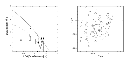
Figure 15: Left:The lateral distribution of charged particles (closed circles) and muons (squares) of the super energetic event recorded by AGASA. The large open circle is the density measured by a detector designed to study the arrival time distribution of particles in air showers. Right: Map of the density distribution of the event. A cross shows the estimated location of the shower core.

Figure 16: Shower longitudinal profile for the highest energy event recorded by the Fly’s Eye.

AGASA would have demonstrated the GZK cutoff were it not for the existence of its most energetic event, whose energy was estimated to be $2.1^{+0.5}_{-0.4}\times 10^{20}$ eV [62]. The details of the event are summarized in table 3. This event hit the array almost at its center, and 23 detectors surrounding the shower core measured local electron densities and shower front arrival time. Detectors more than 2 km away from the core were triggered. Thus, the reconstruction of the lateral distribution of electrons for this event was excellent. The functional fit of the electron density distribution agreed well with all measured densities, which led to an error in the estimation of the charged particle density at 600 meters (S600), of +21 % and -6.6 %. The largest uncertainty in the energy estimation arises from the fact that the attenuation length of S600 as a function of the atmospheric depth is not well known. The zenith angle of this event was $23^{\circ}$. A correction was made to convert the observed S600 to what would be expected for a vertical shower. Although the Monte Carlo prediction suggests that the attenuation effect on S600 is rather moderate, this effect cannot be measured because no other events clearly above 100 EeV have been detected. Furthermore, if this event happened to be observed at the maximum of S600 development, the density at 600 m may not be attenuated at all. Assuming no attenuation gives a lower bound on the primary energy of 170 EeV. This energy is still well beyond the GZK cutoff.

Five muon detectors recorded local muon densities within the dynamic range of the counters. The estimated muon density at 600m from the core is 42.8 m², which agrees well with $31\pm$ 9$m^{2}$ obtained by extrapolation from the lower energy region. There is no clear indication from the EAS muon content that the primary particle is a gamma ray or an extremely heavy nucleus. All that can be claimed concerning this event is that all features including the lateral distribution of electrons, the muon density, and the timing distributions of the particles are consistent with extrapolations from lower energy events.

Table 3: Details of the most energetic events seen by AGASA and Fly’s Eye

	Energy	R. A.	Dec.	Gal.Lat.	Gal.Long.	Zenith Angle	other parameters
AGASA	$2.1\times 10^{20}$ eV	$18.9^{\circ}$	$21.1^{\circ}$	$-41^{\circ}$	$131^{\circ}$	$22.9^{\circ}$	S(600)=892$m^{-2}$
Fly’s Eye	$3.2\times 10^{20}$ eV	$85.2^{\circ}$	$48.0^{\circ}$	$9.6^{\circ}$	$163.4^{\circ}$	$43.9^{\circ}$	$X_{max}=815^{+60}_{-53}g/cm^{2}$

On Oct. 15, 1991, The Fly’s Eye observed an event [63] with an energy of $(3.2^{+0.92}_{-0.94})\times 10^{20}$ eV[64]. This event impacted 13 kilometers away from Fly’s Eye I with a zenith angle of $43.9^{o}$ and an azimuth angle of $31.7^{o}$. At the second site 3.4 km away, the partial eye Fly’s Eye II monitored that half of the visible sky which was in the direction of Fly’s Eye I. Unfortunately, this super high energy event landed on the blind side of Fly’s Eye II, so it was not observed stereoscopically. Nonetheless, the event was particularly well measured by Fly’s Eye I. It fired 22 5.5$\times$5.5^o photomultiplier tubes. The signals were so strong that the high gain channels of several tubes were saturated. The event also has a well-measured longitudinal shower profile. The $X_{max}$ of this event (Fig.16) is estimated to be $815^{+60}_{-53}g/cm^{2}$, with most of the uncertainty coming from the fit of the event geometry. The best estimate of $X_{max}$ falls between that expected for proton and iron showers of this energy. With a single event it is particularly difficult to identify the particle as either proton or iron. Indeed the Fly’s Eye group could not rule out the possibility of the event being a high energy $\gamma$. No strong nearby source is obvious in its arrival direction: right ascension $85.2^{o}\pm 0.5^{o}$, declination $48.0^{o}$ ${}^{+5.2}_{-6.3}$[64]. There are two candidate sources near to the direction of the shower (3C147 & MCG8-11-11), but their distances appear too large for a 320 EeV event to travel[65]. Rachen proposed that 3C134 might be a good candidate but no redshift measurement is available because of the galactic obscuration [66].

If our understanding of the energy estimation on these events is correct, we have another mystery. How could these EHECRs reach earth with such enormous energies? It requires their sources to be remarkably close, less than 50 Mpc, to prevent the expected significant energy loss by the GZK mechanism. Their super-high energies allow the arrival directions to point back to the source locations because the extragalactic magnetic field could not bend their trajectories too much. The upper bound on the deflection angle of a $2\times 10^{20}$ eV event given by equation (4) is only $\sim 1^{\circ}$ for a source distance of 50 Mpc, provided that larger inter-cluster magnetic fields do not actually exist along the propagation path. This is comparable to, or smaller than, the angular resolutions of the experiments. Many searches for possible astronomical sources have been conducted [65], but nothing interesting has been found in the arrival directions of the highest energy particles.

These events may, thus, suggest the appearance of a new population of cosmic rays above the GZK cutoff. This possibility has triggered exotic ideas like the topological defects (“top down”) model [6, 7, 21] and the GRB model [8] which we have already mentioned in this review. The top down model predicted arrivals at earth of gamma rays or protons above the GZK cutoff, with energies originating from GUT scale phenomena. It is difficult to make any claims about the primary composition of the highest energy events. Halzen et al.[67] argued that the Fly’s Eye event could not have been initiated by a photon, based on its shower $X_{max}$. They claimed that a 3$\times 10^{20}$ eV photon initiates an air shower whose peaks at $\sim 940g/cm^{2}$ (without the LPM effect) or $\sim 1075g/cm^{2}$ (with the LPM effect). It should be remarked, however, that the Fly’s Eye shower was a monocular event with an uncertainty in $X_{max}$ of about 60$g/cm^{2}$, mostly caused by uncertainty in geometry. In addition, the reconstruction of this event with deeper $X_{max}$ would lead to lower energy estimation, which decreases the differences between the observation and their Monte Carlo results. Therefore, the Fly’s Eye event by itself cannot rule out the photon origin. On the same note, however, the AGASA event shows normal muon distributions similar to events at lower energies. Thus, these showers are likely to be regular hadronic showers. The GRB model predicts a correlation between the energy and the arrival time, but the current statistics and resolution do not allow a reliable study of this kind of correlation. We should note that the absolute intensity of the flux above the GZK cutoff is consistent with extrapolation of the flux below the cutoff. We cannot give any natural reason why these models give the rate of the super GZK events following the extrapolation.

These arguments concerning the “new” population of cosmic rays are based mainly on these two events. Although the groups have carefully analyzed the data, and nothing has been found to cause unreasonable overestimation of energies in these events, we should not neglect the possibility that an unpredicted tail of the energy resolution may have given rise to these remarkable energies. The energy estimation of the AGASA events relies mostly on Monte Carlo studies and extrapolation of the observed behavior in the lower energy region. The Fly’s Eye event was a monocular one (viewed only by a single eye). Detection of more super-GZK events with reliable energy estimation is required in order to say more about this class of events. In addition, it is important to increase number of events between $10^{19}$ and $10^{20}$ eV which are able to “calibrate” our energy estimation for these highest energy events.

7 Absolute energy calibration and energy resolution

Before we leave the energy spectrum, we must discuss the absolute energy calibration and energy resolution of the experiments.

One question about the Fly’s Eye energy determination is the absolute efficiency for the production of fluorescence light. All Fly’s Eye analysis are based on the efficiency estimate compiled by Bunner[68]. A recent measurement of the scintillation efficiency has been conducted by Kakimoto et al[69]. The Fly’s Eye group have compared the event energies using Bunner’s efficiency and the new efficiency, and have found the difference to be only about 1% [70].

The insensitivity of the $\rho(600)$ to the interaction model does not exempt its model dependence totally. The MOCCA (or pre-MOCCA) models[49] used by the Haverah Park experiment, no doubt represented the best knowledge of hadronic interactions in the 1970’s, however recent Fly’s Eye, AGASA and Yakutsk data favor models which are more consistent with a quicker dissipation of energy (faster than the scaling models used by Haverah Park) [71, 72, 73]. Evidence shows that the MOCCA program, which was used to determine the relation between the primary energy and $\rho(600)$, underestimates the muon density by almost a factor of two at large distances from the core for showers between 10¹⁸ and 10¹⁹ eV. A water Cherenkov detector is more sensitive to muons compared with very soft electrons far from the shower core. As discussed by Lawrence, Reid, and Watson [31], the overestimation in energy could be as large as 40% if, indeed, the high dissipation model is correct. The 40% will certainly reduce the disagreement between Haverah Park and the other experiments in terms of the number of events above $10^{20}$eV per unit exposure (see table 2). This would make the Haverah Park result more comparable with a GZK cutoff. We have seen arguments that the systematics in energy calibration among experiments are much smaller than 40%, based on the flux differences. However, the aperture calculation and the energy resolution have a large effect on the estimated flux. The flux can be significantly underestimated near the detector threshold energy. This is because there are no events below the threshold energy that trigger the array and are reconstructed to have an energy higher than their true energy. On the other hand, showers just above the threshold can have reconstructed energies above their true energy, and rob the threshold area of flux due to the familiar “downhill” effect.

We must also emphasize the importance of resolution. The effect can easily be demonstrated by observing the difference between the Fly’s Eye monocular spectrum (Fig.14) and the stereo spectrum (Fig.7). Due to the poorer resolution, the “dip” structure in the monocular spectrum is much less striking than that in the stereo spectrum. The apparent “dip” position is also shifted to nearly $10^{18.9}$ eV. The relative energy calibration between the monocular and stereo events has been carefully balanced using the stereo events, hence the shift in the ’dip’ position is entirely due to the effect of resolution.

8 Chemical composition

8.1 Composition from $X_{max}$ measurements

The position of shower maximum in the atmosphere ($X_{max}$) in $g/cm^{2}$ is sensitive to the composition of the primary particle. Protons for instance, will on average experience their first interaction deeper in the atmosphere than heavy nuclei of the same energy. Proton showers are also expected to develop more slowly than heavy primary showers with the same energy per primary particle. The primary chemical composition can be, therefore, deduced from the distribution of $X_{max}$.

The Fly’s Eye group derive their composition estimate by comparing the measurements with Monte Carlo predictions. The Monte Carlo showers are generated using a QCD Pomeron model ( the so-called KNP model) [71, 74]. The Monte Carlo generated showers are then passed through the detector Monte Carlo simulation program to account for detector trigger biases. Those events triggering both Fly’s Eye sites in the detector Monte Carlo are written to a data file with the same format as the real data. This fake data set is then reconstructed using the same programs used in the real data analysis.

Figure 17: The $X_{max}$ elongation rate. Black dots: Fly’s Eye data. Open squares : proton $X_{max}$ distribution based on the KNP model. Open circles: iron $X_{max}$ distribution based on the KNP model. Diamonds: expected mean $X_{max}$ distribution based on a simple two component model.

The mean X_max as a function of primary energy measured by the Fly’s Eye detectors, is shown in Fig.17 together with KNP model Monte Carlo generated proton and iron showers. From the figure, one can see that the composition is heavy at a few times 10¹⁷ eV and gradually shifts to light primaries near 10¹⁹eV. The same conclusion is reached by comparing the rise and fall of the full X_max distributions in each energy bin [75]. The elongation rate (the increment of $X_{max}$ per decade of energy) from 0.3 EeV to 10 EeV is 78.9$\pm$3$g/cm^{2}$ per decade for the real data, and 50 $g/cm^{2}$ per decade for the Monte Carlo simulated proton or iron showers.

Constraints on hadronic interaction models by the Fly’s Eye measurements arise from the fact that the Fly’s Eye measures both the absolute $X_{max}$ position at each energy and the elongation rate. The absolute mean value of $X_{max}$ around $3\times 10^{17}$ eV (about 630$g/cm^{2}$) essentially rejects any model with a large elongation rate, since those large elongation rate models inevitably predict a deeper $X_{max}$ at $3\times 10^{17}$ eV, even with an iron primary.

The facts that the measured absolute value of $X_{max}$ at $3\times 10^{17}$ eV is low and that the measured elongation rate is high, naturally leads to the conclusion that the composition is becoming lighter over the energy range observed. Of course, a quantitative prediction of how quickly the composition gets lighter is still model dependent.

A recent result from the HiRes prototype detector supports the conclusion that the composition around $3\times 10^{17}$ eV is heavy[76]. In addition, event reconstruction using the new air scintillation efficiency (mentioned earlier) does not affect the original Fly’s Eye composition conclusion.

Figure 18: The Yakutsk mean $X_{max}$ as a function of primary energy. Solid lines are the Monte Carlo predictions of a QCD pomeron model from the Fly’s Eye group. The dashed line is the fit to points above $1.1\times 10^{18}$ eV.

Yakutsk derives the depth of shower maximum using the Cherenkov lateral distribution[77, 51]. Parameters used to get $X_{max}$ are the ratio of the Cherenkov flux to the charged particle size, the Cherenkov lateral distribution slope at core distances between 100 and 400 m, and a characteristic radius, $R_{o}$, determined by the Cherenkov light between 50 and 300 m from the core [77]. Further communication from the Yakutsk group is still necessary to fully understand how these parameters are used to derive $X_{max}$. Fig.18 shows the derived $X_{max}$ as a function of primary energy[51]. We realized at the time of writing this paper, that the Monte Carlo predictions in the Yakutsk $X_{max}$ plot are digitized from the Fly’s Eye $X_{max}$ plot. Around $10^{17}$ eV, the Yakutsk group claim their $X_{max}$ values indicate that the composition is mixed. They further claim that as energy increases the composition gets lighter. The QCD Pomeron elongation rate is about 50$g/cm^{2}$ per decade over this energy range. The measured elongation rate is $79\pm 3g/cm^{2}$ per decade for events above 1.1$\times 10^{18}$ eV[51]. But we need to be very careful here since the Monte Carlo predictions include the Fly’s Eye detector bias and the Yakutsk Cherenkov detector does not necessarily have the same detector bias as the Fly’s Eye fluorescence detector. We do notice that a qualitative conclusion which agrees with the above picture has been drawn by the same group[50]. In this case, the conclusion is based on the QGS[78] model, but no plot is shown. The typical separation in mean $X_{max}$ between proton and iron showers is about 75 to 100 $g/cm^{2}$ in this energy range, and the detector bias could be as large as 20 or 30$g/cm^{2}$. Therefore, we encourage the Yakutsk group to carry out their own detector Monte Carlo simulations when comparing their data with predictions.

8.2 Composition from muon to electron ratio

The AGASA experiment has measured the muon density as a function of the primary energy of cosmic rays or rather as function of S600, their observable energy estimator. Their results at higher energies are very consistent with that expected from extrapolation of data in the lower energy region. They measured the slope of the logarithm of muon density to that of electrons and found that this slope does not change for E$\geq 10^{17.5}$ eV. They used the MOCCA event generator package [49] to find that the Fly’s Eye’s picture should have caused a change in the slope [79]. It is claimed that there is no evidence in the AGASA measurement to support the Fly’s Eye result of a change in the chemical composition.

Figure 19: The ratio of charged particle size to muon size (muon threshold 1 GeV) as a function of the primary energy from the Yakutsk experiment. Solid lines are the Monte Carlo predictions of the QGS model (Upper curve: proton, lower curve: iron). Dashed lines are the Monte Carlo predictions of a scaling model(Upper curve: proton, lower curve: iron).

In addition to the Cherenkov lateral distribution, the Yakutsk group also measure muon densities. Instead of plotting muon size against the all charged particle size as is usually seen, the reverse is plotted in Fig.19. Two model predictions are plotted in the same figure, one uses the QGS model [78], and the other uses an old-fashioned scaling model[80]. It is interesting to note that the QGS model predicts a charged particle to muon ratio which is more than a factor of two smaller than the scaling model prediction at energies above $10^{18}$ eV. The Yakutsk group reach the same conclusion as the Fly’s Eye about the composition as their $X_{max}$ result, if the QGS model is used to interpret the data. On the other hand, the scaling model predicts fewer muons, and prefers a flux of almost 100% iron below $10^{18}$ eV before running into difficulty above $10^{18}$eV where a composition heavier than iron is required. Here again we emphasize the importance of a detector Monte Carlo. It is vital to take the detector bias into account when comparing with Monte Carlo predictions.

8.3 Effort in unifying the composition results

Figure 20: The muon density at 600 meters from shower core as a function of the primary energy from the Akeno A1 array. The lines are the predictions of ’Sibyllized MOCCA’. Dotted line: iron primaries. Dashed line: proton.

The apparent contradiction between the Fly’s Eye $X_{max}$ measurement and the AGASA muon to electron ratio measurement draws much attention. The interaction model (contained in the original MOCCA) used by AGASA to interpret the muon data was immediately questioned. From the absolute $X_{max}$ position at low energy (3$\times 10^{17}$eV), the Fly’s Eye group and their model providers [71, 72] realized that no scaling model fits the data at this energy. A model with a higher rate of energy dissipation, either through large cross-section or through large inelasticity, or both, is required. Such a fast energy dissipation model leads to the rapid development of showers, smaller depth of shower maximum ($X_{max}$) and a smaller elongation rate (the increment of $X_{max}$ per decade of energy). Hence, in terms of shower development, a proton shower will asymptotically approach a “conventional” iron shower, where “conventional” means an extrapolation from lower energy behavior using a scaling model. Similarly, in terms of muon content proton showers will become more and more like conventional iron showers, since both $X_{max}$ and the muon content are related to the distributions of secondary particle energies.

This inspired a group of people from Adelaide (Dawson et. al. [81]) to perform a cross check using the so called “Sibyllized MOCCA”, which uses the MOCCA program as the shower driver, but uses the Sibyll model[73] for the hadronic interactions. Their simulations show that while exact fractions of protons and iron derived from the Fly’s Eye measurements of $X_{max}$ are somewhat model dependent, there is still clear evidence that the composition is changing from heavy to light. The elongation rate from this model is smaller than that predicted by the original MOCCA code (without Sibyll). This has a related effect for muons: the newer model gives a steeper slope to the muon content as a function of energy. In fact the proton slope is even steeper than that for iron at the same energy per primary particle. The energy per nucleon for protons is 56 times that of iron. With the Sibyll model the AGASA muon measurement no longer contradicts a changing composition (see Fig.20).

As a by-product of composition measurements, it is now believed that the cascade of nucleon-nuclei interactions dissipates energy faster than the scaling models would predict using an extrapolation from lower energies.

To summarize the composition measurements, we have seen that the Fly’s Eye $X_{max}$ measurements indicate that the composition is shifting from heavy to light over the energy range from $10^{17}$ eV to $10^{19}$ eV. At Yakutsk, both the $X_{max}$ and the muon density results favor a composition change from a mixture of heavy and light to light over the same energy region, however, a detector Monte Carlo is needed to strengthen their conclusions.

While the original analysis of the AGASA muon measurement states that there is no indication of a changing composition, the application of a consistent hadronic model brings the results into better agreement with the Fly’s Eye conclusion. In terms of the composition, the Fly’s Eye results support a two component picture where a heavy flux is progressively dominated by a protonic flux at higher energies. Yakutsk does not support the first component being very heavy, but does favor a light second component. AGASA cannot be regarded as supportive of a two component picture, based on their original analysis, but there may be room for a consensus if conclusions are based on similar hadronic models. It is clear, however, that better measurements and a further refinement of interaction models are necessary to resolve the composition issue.

9 Anisotropy

Figure 21: Arrival directions (in galactic coordinates) of EHECRs above $10^{19}$ eV detected by AGASA.

Results from all experiments indicate that cosmic ray arrival directions are largely isotropic. Typical upper bounds on the amplitude of the anisotropy (first and second harmonics in right ascension) are less than 5% for events around $10^{18}$ eV, less than 10% for events around $10^{18.5}$ eV and less than 30% for events around $10^{19}$eV[82]. Lee and Clay[83] have argued that, based on the amplitudes of the harmonics, cosmic rays in this energy range cannot be protons originating within the galaxy.

Based on a data set mainly from Haverah Park, Stanev et al[84] pointed out that the arrival directions of cosmic rays with energies above $4\times 10^{19}$eV (a total of 42 events) exhibit a correlation with the general direction of the supergalactic plane, a plane defined by nearby radio galaxies ($z\leq 0.02$) in the northern hemisphere. The chance probability that a uniform distribution would have such a concentration is a few percent, according to their simulation. This concentration diminishes as the cosmic ray energy goes down. There is no galactic plane enhancement (the same analysis actually indicates that cosmic rays above $4\times 10^{19}$ eV are more likely to come from large galactic latitudes). Kewley, Clay, and Dawson[85] applied the same analysis to the southern part of the sky using data from the Sydney SUGAR array [28] and no concentration around the supergalactic plane was found. This may be because the plane is less well defined in the south.

Figure 22: Arrival directions in galactic coordinate of EHECRs above $4\times 10^{19}$ eV recorded by AGASA (Open squares – $E\geq 5\times 10^{19}$ eV, open circles – $5\times 10^{19}$ eV $\geq E\geq 4\times 10^{19}$ eV). The dashed curve shows the supergalactic plane. The cross hatched area represents parts of the sky unobservable by AGASA.

Figure 21 shows the arrival directions of all EHECRs recorded by AGASA with energies above $10^{19}$ eV. The distribution is completely consistent with an isotropic distribution [86]. No evidence of enhancement associated with the galactic plane has been detected and the group did not find significant enhancement along the supergalactic plane [87]. However, an interesting feature has been reported [87]: event clusters. Figure 22 shows the arrival directions of EHECRs above $4\times 10^{19}$ eV recorded by AGASA. Three event pairs each with angular separations of less than $2.5^{\circ}$ have been detected. Two of the pairs are within $2^{\circ}$ of the supergalactic plane. The chance probability of having two or more such pairs has been estimated to be $2.9\times 10^{-2}$.

None of these pairs arrive from our galactic plane again favoring the extragalactic origins of EHECRs. However, these features themselves contain some mysteries. First, the AGASA group have found no active astrophysical objects in the directions of the pairs. The threshold of $4\times 10^{19}$ eV requires sources within $\sim 500$ Mpc [14] because of the energy loss in the microwave background field. Some Markarian-type galaxies have been found, but no FR II type radio galaxies. Second, if these events are protons, then possible extragalactic magnetic fields should bend their trajectories, which would result in a larger separation angle between the two events in a pair. Equation (4) gives 6.8^∘ for sources at a distance of 80 Mpc (corresponding to radio galaxies in the supergalactic plane) and 17^∘ for those at 500 Mpc (the upper bound on the distance of possible sources). To explain the observed angular separation, then either the extragalactic magnetic field must be much lower than the current upper bound given in equation (3), or the primary particles in these events must be neutrally charged, perhaps photons. The observed muon densities in these events are, however, consistent with hadron primaries.

We should note here that this kind of analysis might be criticized in terms of the uncountable degrees of freedom in the estimation of the statistical significance. There is no clear reason why an angular separation of 2.5^∘ should be chosen to define an event pair. It has been claimed that this number is consistent with the experimental angular resolution, but $2^{\circ}$ or 3.5^∘ instead of 2.5^∘ would be just as consistent, within uncertainties, in the angular resolution, which vary from event to event. Furthermore, a search for event clusters with a larger angular separation might also be reasonable given the possible bending of trajectories by the extragalactic field. If the angular separation can be considered as a free parameter, the chance probability of 2.9% might be too weak to claim the existence of the pairs. The same attention should be paid to the combined analysis of the different experiments by Uchihori et.al. [88]. They claimed a possible correlation of the event clusters (including triplets) and the supergalactic plane with a significance level of a few percent. It is true that the pooling of results from different experiments is a vital effort aimed at overcoming the limitation of poor statistics, but the problem of dealing with data sets with different angular resolutions makes it difficult to draw a reliable conclusion. In contrast to the angular separation, the choice of the threshold energy of $4\times 10^{19}$ eV in the analysis can be justified since this energy is the universal value marking the beginning of the GZK cutoff in the spectrum.

10 Summary

The EHE cosmic ray energy spectrum steepens in the energy region between $10^{17.6}$ and $10^{18}$eV (the second “knee”, where the spectral slope changes from -3.0 to -3.3) and flattens between $10^{18.5}$ and $10^{19}$ eV (the so called “ankle”, where the spectral slope changes from -3.3 to approximately -2.7). The straightforward, and less model-dependent, interpretation is a two component scenario: a high energy extragalactic component dominates over a steeper galactic component above the ankle. The many experimental results now available are supportive of this picture, including: a possible signature of the GZK cutoff obtained by the Fly’s Eye, AGASA and Yakutsk; an indication of the chemical composition getting lighter at high energies from the Fly’s Eye and Yakutsk groups; no enhancement of the arrival direction distribution associated with the galactic plane; a possible correlation with the supergalactic plane found in a combined data set mainly consisting of Haverah Park data; and three event clusters above $4\times 10^{19}$ eV observed by AGASA arriving from directions well away from the galactic plane.

Although our two component picture seems to make sense when we put these results together, the conclusion is far from solid. The significance of the GZK cutoff is muddied by the super-high energy events well beyond the cutoff, thereby providing complications to the simple picture of the GZK mechanism. The interpretation of chemical composition measurements has some model dependence as cautioned by the AGASA results. The statistical significance of the event clusters only allows us to suggest possible “hints” of something exciting. What encourages us about the two component scenario is the fact that different analysis from different experiments seem to be reasonably consistent under our scenario. The next step is to make all these results robust by accumulating more data with good resolution. For example, a fine measurement of the GZK cutoff would clarify the extragalactic hypothesis. A clear measurement of the mass composition above the “ankle” would also be very helpful in confirming or rejecting our current picture. A detection of a EHE photon or neutrino component would bring us a new understanding of the universe. During the next decade, we will see the study of EHE cosmic rays continue to provide a laboratory for non-accelerator particle physics, and we look forward to it establishing a new astronomy.

Acknowledgments

The authors are grateful to B. Dawson, P. Sommers, P. Sokolsky, M. Teshima, J. N. Matthews, and G. B. Yodh for helpful suggestions and advice. They also wish to thank M. Nagano for allowing us to use the preliminary analysis by one of the authors (S.Y.) based on the published data from the AGASA experiment.

References

- [1] Drury L O’C 1991 in Astrophysical aspects of the most energetic cosmic rays edited by M. Nagano and F. Takahara p.252 (World Scientific, Singapore)
- [2] Hillas A M, 1984, Ann.Rev.Astron.Astrophys. 22 425
- [3] Ip W H and Axford W I, 1991 in Astrophysical aspects of the most energetic cosmic rays edited by M. Nagano and F. Takahara p.273 (World Scientific, Singapore)
- [4] Mannheim, K., 1995, Astropart.Phys., 3, 295
- [5] Rachen, J P, and Biermann, P L, 1993, Astron.& Astrophys, 272, 161
- [6] Bhattacharjee, P., Hill C.T., and Schramm D.N., 1992, Phys.Rev.Lett., 69, 567
- [7] Bhattacharjee P and Sigl G, 1995, Phys. Rev. D51, 4079.
- [8] Waxman, E., 1995, Phys.Rev.Lett., 75, 386
- [9] Vietri M, 1995, Astrophys. Journal, 453, 883
- [10] Kronberg P P, 1994, Rep.Prog.Phys., 57, 325
- [11] Waxman E, and Miralda-Escudé L, 1996, Astrophys Journal, 472, L89
- [12] Greisen K 1966 Phys. Rev. Lett. 16, 748.
- [13] Zatsepin G T, & Kuzmin V A 1966, Sov.Phys. JEPT Lett. 4, 78.
- [14] Yoshida S and Teshima M, 1993, Prog. Theor. Phys. 89, 833.
- [15] Protheroe R J and Johnson P, 1996, Astropart. Phys. 4, 253.
- [16] Puget J L, Stecker F W & Bredekamp J H, 1976, Astrophys. Journal. 205, 638.
- [17] Sigl, G, Lee, S., Coppi, P., 1996 astro-ph/9604093, submitted to Phys.Rev.Lett.
- [18] Lee S, 1996, astro-ph/9604098, submitted to Phys.Rev.D.
- [19] Hill C T, and Schramm, D N, 1983, Phys.Lett., 131 B, 247
- [20] Yoshida S, et al., 1997, Astrophys. Journal, 479, 547
- [21] Sigl, G., Lee, S., and Schramm, D. N., 1997, Phys.Lett. 392 B, 129
- [22] Roulet E, 1993, Phys.Rev.D 47, 5247 (1993)
- [23] Yoshida S, 1994, Astropart.Phys. 2, 187
- [24] Weiler, T J, preprint VAND-TH-97-8, hep-ph/9710431
- [25] Linsley J. 1963a, Phys. Rev. Lett. 10, 146.
- [26] Linsley J. 1963b, Proc.8th Int. Cosmic Ray Conf. 4, 295.
- [27] Brownlee R G et al, 1968, Can. J. Phys. 46, S259.
- [28] Winn M M et al, 1986, J. Phys. G, 12, 653.
- [29] Watson A A 1991, Proc. 12th European Cosmic Ray Symp. (Nottingham) Nucl.Phys. B Suppl. 22B, 116.
- [30] Lawrence M A, Reid R J O, & Watson A A 1990, Proc. 21st Int. Cosmic Ray Conf. 3, 159.
- [31] Lawrence M A, Reid R J O, & Watson A A 1991, J. Phys. G: Nucl. Part. Phys., 17, 733.
- [32] Efimov N N, Egorov T A, Glushkov A V, Pravdin M I, & Sleptsov, I Y 1991, Proc. Int. Symp. on Astrophysical Aspects of the Most Energetic Cosmic Rays, ed. M. Nagano & F. Takahara (Singapore World Scientific), 20.
- [33] Baltrusaitis R M et al. 1985a, Nuclear Instruments and Methods, A240, 410.
- [34] Baltrusaitis R M et al. 1985b, Physical Review Letters, 54, 16, 1875.
- [35] Nagano M et al. 1992, J. Phys. G: Nucl. Phys., 18, 423.
- [36] Yoshida S et al., 1995 , Astropart.Phys. 3, 105
- [37] Takeda, M 1997 Private Communications
- [38] Abu-Zayyad T et al 1997a, Proc. 25th ICRC, 5, 321.
- [39] Abu-Zayyad T et al 1997b, Proc. 25th ICRC, 5, 325.
- [40] Abu-Zayyad T et al 1997c, Proc. 25th ICRC, 5, 329.
- [41] Cronin J W, 1992, Nucl. Phys. 28B (Proc. Supp.), 213.
- [42] The Auger Collaboration, 1997, Pierre Auger Project Design Report, 2nd Edition.
- [43] Boratav M et al 1997, Proc. 25th ICRC, 5, 205.
- [44] Dawson B R, Fick B E, Kampert K H and Sommers P, 1997, Proc. 25th ICRC, 5, 377.
- [45] Aiso S et al 1997a, Proc. 25th ICRC, 5, 369.
- [46] Aiso S et al 1997b, Proc. 25th ICRC, 5, 373.
- [47] Ormes J F et al 1997, Proc. 25th ICRC, 5, 273.
- [48] Linsley J et al 1997, Proc. 25th ICRC, 5, 385.
- [49] Hillas A M, Marsden D J, Hollows J D and Hunter H W, 1971, Proc. 12th ICRC, Hobart, 3,1001.
- [50] Afanasiev B N et al, 1996, Proc. Int. Symp. on Extremely High Energy Cosmic Rays: Astrophysics and Future Observatories, Ed. by M. Nagano, p.32.
- [51] Egorov T A, 1993, Proc. Tokyo Workshop on Techniques for the Study of Extremely High Energy Cosmic Rays, ICRR, University of Tokyo, 35.
- [52] Ohoka, H et al 1997 Nucl.Inst.Meth. A 385, 268
- [53] Yoshida S, et al., 1994 J.Phys.G:Nucl.Part.Phys. 20 651
- [54] Cassiday G L 1985, Ann. Rev. Nucl. Part. Sci. 35, 321.
- [55] Bird D J et al, 1993, Phys. Rev. Lett. 71, 3401.
- [56] Bird D J et al, 1994, Astrophys. Journal 424, 491.
- [57] Cunningham G et al, 1980, Astrophys. Journal 236, L71.
- [58] Afanasiev B N et al, 1995a, Proc. 24th ICRC, 2, 756.
- [59] Sokolsky P, Sommers P and Dawson B R, 1992, Physics Reports, 217, 225.
- [60] Hayashida N et al., 1997, Proc. ICRC International Symp. on Extremely High Energy Cosmic Rays. 402.
- [61] Berezinsky V S, and Grigor’eva S I, 1988, Astron.& Astrophys 199 1.
- [62] Hayashida N, et al. 1994, Phys.Rev.Lett. 73, 3491
- [63] Loh E C, 1993, Proc. Tokyo Workshop on Techniques for the Study of Extremely High Energy Cosmic Rays Ed. by M. Nagano, p.52.
- [64] Bird D J et al, 1995, Astrophys. Journal 441, 144.
- [65] Elbert J W and Sommers P, 1995, Astrophys. Journal 441, 151.
- [66] Rachen J P, 1994 Proc.17th Texas Symposium on Relativistic Astrophysics (Munich, 11-17 Dec 1994).
- [67] Halzen F et al, 1995, Astropart. Phys. 3, 151.
- [68] Bunner, A. N., PhD Thesis, Cornell University, 1967.
- [69] Kakimoto T et al, 1996, Nuclear Instruments and Methods A 372, 527.
- [70] Loh E C & Dai H Y, 1996, Proc. Int. Symp. on Extremely High Energy Cosmic Rays: Astrophysics and Future Observatories, Ed. by M. Nagano, p.28.
- [71] Gaisser T K et al, 1993, Phys. Rev. D47, 1919.
- [72] Ding L K et al, 1997, Astrophys. Journal 474, 490.
- [73] Fletcher R S et al, 1994, Phys. Rev. D50, 5710.
- [74] Kopeliovich N N, Nikolaev N N, & Potashnikova I K 1989, Phys. Rev. D, 39, 769.
- [75] Sokolsky P et al, 1993, Proc. 23rd ICRC, Invited, Rapporteur & Highlight Papers, 447.
- [76] Kidd J M, 1997, PhD Thesis, University of Illinois at Urbana-Champaign.
- [77] Dyakonov M N et al, 1993, Proc. 23rd ICRC, 4, 303.
- [78] Kalmykov N N et al, 1995, Proc. 24th ICRC, 1, 123.
- [79] Hayashida N, et al. 1995, J.Phys.G:Nucl.Part.Phys. 21, 651
- [80] Elbert J W & Gaisser T K, 1979, Proc. 16th ICRC, 8, 42.
- [81] Dawson, B.R., Meyhandan, R., and Simpson, K.R., 1998, astro-ph/9801260, submitted to Astropart.Phys.
- [82] Teshima M, 1993, Proc. 23rd ICRC, Invited, Rapporteur & Highlight Papers, 257.
- [83] Lee A A & Clay R W, 1995, J.Phys.G:Nucl.Part.Phys. 21, 1743
- [84] Stanev T et al, 1995, Phys. Rev. Lett. 75, 3056.
- [85] Kewley L J, Clay R W & Dawson B R, 1996, Astropart. Phys. 5, 69.
- [86] Hayashida, N., et al., 1997, Proc. 25th ICRC 4, 177
- [87] Hayashida, N., et al., 1996, Phys.Rev.Lett. 77, 1000
- [88] Uchihori Y et al, 1996, Proc. Int. Symp. on Extremely High Energy Cosmic Rays: Astrophysics and Future Observatories, Ed. by M. Nagano, p.50.