Dust grains and the structure of steady C-type magnetohydrodynamic shock waves in molecular clouds

Abstract

I examine the role of dust grains in determining the structure of steady, cold, oblique C-type shocks in dense molecular gas. Gas pressure, the inertia of the charged components, and changes in ionization are neglected. The grain charge and rate coefficients for electron-neutral and grain-neutral elastic scattering are assumed constant at values appropriate to the shock interior. An MRN size distribution is accounted for by estimating an effective grain abundance and Hall parameter for single-size grains.

A one-parameter family of intermediate shocks exists for each shock speed $v_{s}$ between the intermediate signal speed $v_{A}{\rm cos}\theta$ and $\sqrt{2}v_{A}{\rm cot}\theta$, where $v_{A}$ is the pre-shock Alfvén speed and $\theta$ is the angle between the pre-shock magnetic field and the normal to the shock front. In addition, there is a unique fast shock for each $v_{s}>v_{A}$.

If the pre-shock density ${n_{\rm H}}\ga 10^{5}\,\mathrm{cm}^{-3}$ and the pre-shock magnetic field satisfies $B(\mathrm{mG})/{n_{\rm H}}(10^{5}\,\mathrm{cm}^{-3})\la 1$ grains are partially decoupled from the magnetic field and the field and velocity components within fast shocks do not lie in the plane containing the pre-shock field and the shock normal. The resulting shock structure is significantly thinner than in models that do not take this into account. Existing models systematically underestimate the grain-neutral drift speed and the heating rate within the shock front. At densities in excess of $10^{8}\,\mathrm{cm}^{-3}$ these effects may be reduced by the nearly-equal abundances of positive and negative grains.

1 Introduction

The structure of shock waves in molecular clouds is determined by the coupling between the magnetic field and the weakly ionized pre-shock gas. For shock speeds below 40–50 $\,\mathrm{km\,s}^{-1}$ (McKee, Chernoff & Hollenbach 1984) Lorentz forces within the shock front push the charged species through the neutrals, and the resulting collisions accelerate, compress, and heat the ambient gas. This process is slow because the charged species are rare, so the gas is able to radiate away a significant fraction of the heat while still within the shock front (Mullan 1971; Draine 1980), primarily through the emission of radiation in molecular rotational and vibrational transitions. Shocks of this nature are denoted ‘C-type’ (Draine 1980), or ‘C^∗-type’ if the gas is decelerated through a sonic point in the reference frame comoving with the shock front (Chernoff 1987, Roberge & Draine 1990). At higher shock speeds, the molecular coolants are dissociated, cooling can no longer keep pace with heating, and the gas pressure becomes dynamically significant. A thin, viscous sub-shock forms within the front, and the shock is termed ‘J-type’ (Draine 1980).

C-type shocks efficiently convert the heat produced by collisions within the shock front into molecular line emission, and are responsible for much of the intense infrared H₂ and CO line emission observed towards the Orion-KL region (Draine & Roberge 1982; Chernoff, McKee & Hollenbach 1982; Smith & Brand 1990; Smith, Brand & Moorhouse 1991; Chrysostomou et al. 1997). The warm molecular environment within C-shocks can drive molecular chemistry such as the conversion of atomic oxygen into OH and then into water (Draine, Roberge & Dalgarno 1983; Kaufman & Neufeld 1996a,b). In addition, the large drift speeds can drive exothermic ion-neutral chemistry within the shock front (Flower, Pineau des Fôrets & Hartquist 1985; Pineau des Fôrets, Flower & Hartquist 1986; Draine & Katz 1986a,b).

Shock models have generally been forced to be ‘coplanar’, that is, the drift velocities and magnetic field within the shock front are assumed to lie in the ‘shock plane’, the plane containing the pre-shock magnetic field and the shock normal (see Fig. 1). This holds for fast shocks if the charged species are tied to the field lines, but charged grains drift obliquely to the shock plane if they become partially decoupled from the field lines by collisions with the neutrals (Draine 1980). However, for the sake of simplicity, the component of the grain drag force on the neutrals perpendicular to the shock plane has usually been supressed (e.g. Draine et al. 1983; Wardle & Draine 1987). This approximation breaks down for high pre-shock densities, partly because the fractional ionization of the gas decreases, permitting the grains to make a larger fractional contribution to the drag on the neutral gas, but also because the grains become poorly coupled to the magnetic field and the grain drag vector is further tilted out of the shock plane.

This motivated calculations of the structure of grain-dominated C-shocks in which the vector components perpendicular to the shock plane were retained. Pilipp, Hartquist & Havnes (1990) showed that the thickness of perpendicular shocks was significantly changed for pre-shock densities in excess of $10^{7}\,\mathrm{cm}^{-3}$. In this case, the symmetries of the geometry constrain the magnetic field direction to be the same throughout the shock front, even though the drift velocities need not lie within the shock plane.

Oblique shocks introduce an important extra degree of freedom, in that $\mn@boldsymbol{B_{\perp}}$, the magnetic field component perpendicular to the shock normal, may rotate within the shock front before returning to the shock plane downstream. Oblique shocks were studied by Pilipp & Hartquist (1994), who found solutions for shock speeds below a few $\,\mathrm{km\,s}^{-1}$ in which $\mn@boldsymbol{B_{\perp}}$ rotates by 180°(in either sense) within the shock front. Pilipp & Hartquist were unable to find solutions for shock velocities in excess of a few $\,\mathrm{km\,s}^{-1}$, and suggested that steady shock solutions may not exist in this regime. This is disconcerting, as shocks with speeds in excess of 20 $\,\mathrm{km\,s}^{-1}$ are required to model the observed emission from a variety of sources. In addition, the development of a sound theoretical understanding of magnetohydrodynamics of dense, dusty gas is important for scenarios for the formation and collapse of molecular cloud cores and the formation of protostellar discs (e.g. Nishi, Nakano & Umebayashi 1991; Ciolek & Mouschovias 1993; Neufeld & Hollenbach 1994; Li & McKee 1996; see also the review by Hartquist, Pilipp & Havnes 1997).

The behaviour of $\mn@boldsymbol{B_{\perp}}$ in the solutions obtained by Pilipp & Hartquist is fundamentally different to the earlier coplanar oblique shock models (Wardle & Draine 1987; Wardle 1991a; Smith 1992), in which the pre-shock and post-shock $\mn@boldsymbol{B_{\perp}}$ vectors are parallel rather than antiparallel. The upstream and downstream states across magnetohydrodynamic (MHD) shocks are related by jump conditions that are independent of the detailed nature and behaviour of the fluid, and therefore of the actual shock structure. In particular, the transverse magnetic field increases, changes sign, or decreases across the fast, intermediate, or slow shocks respectively (e.g. Cowling 1976; Kennel, Blandford & Coppi 1989). This implies that the solutions found by Pilipp & Hartquist are C-type intermediate shocks, whereas previously studied C-shock solutions are fast shocks. The jump conditions show that the downstream state for intermediate shocks is unphysical for shock speeds a little above the Alfvén speed, and this explains the breakdown of the solutions for mildly super-Alfvénic shocks. Further, for a given shock speed, Pilipp & Hartquist found a one-parameter family of shock solutions rather than the single shock solution found in previous studies, and noted that this has also been found to be the case for intermediate shocks in resistive MHD (Wu 1988a; Kennel, Blandford & Wu 1990).

Having identified these solutions as intermediate shocks, there still remains the important issue of the existence of fast shock solutions. On grounds of physical continuity, one expects that adding grains to a coplanar, fast C-type shock should distort the structure out of the shock plane rather than do away with it entirely. Indeed, there are hints that steady shock solutions may exist. Following standard practice in C-shock modelling, Pilipp & Hartquist derived a set of ODE’s describing the shock structure, and integrated them from a perturbed upstream state towards the shock front. There is, however, a difference in the number of free parameters describing the initial perturbed state. In the coplanar case there is one free parameter – the amplitude of the initial perturbation in the pre-shock fluid (Draine 1980; Wardle & Draine 1987). Physically, this specifies the point in the shock precursor at which the integration towards the shock front begins, so there is a single shock solution for a given shock speed, the fast shock. Dropping the assumption of coplanarity introduces a second parameter, which can be regarded as the degree of rotation of the perturbation out of the shock plane at the initial point. The freedom introduced by the new parameter potentially allows a family of solutions to exist (the intermediate shocks), and Pilipp & Hartquist found that there is a critical value at which the sense of rotation of $\mn@boldsymbol{B_{\perp}}$ across the intermediate shock solutions changes sign. This suggests that the fast shock solution corresponds to this critical value, but that the solution cannot be found by integration from the perturbed upstream state because of finite numerical precision.

This paper demonstrates that fast non-coplanar C-shock do exist. As the issues addressed here are fundamental in nature, I keep the formulation of the multifluid shock problem, described in the next section, as simple as possible. In particular, I assume that the molecular gas consists of four distinct species: neutrals, positive ions, electrons or PAHs, and negatively charged grains. Gas pressure is neglected, and ionization balance and chemistry are also ignored. These simplifications allow all of the physical quantities in the shock to be expressed in terms of the components, $B_{x}$ and $B_{y}$, of $\mn@boldsymbol{B_{\perp}}$. Thus a shock solution can be represented by a plot of $B_{y}(z)$ vs. $B_{x}(z)$, where $z$ is the coordinate along the shock normal. This two-dimensional phase space, explored in §3, is a powerful tool for examining the set of shock solutions given the pre-shock conditions and shock speed. In §4 I show that both fast and intermediate shock solutions exist for low shock speeds, and that the topology of the phase space prevents the fast shock solution from being found by integration from upstream to downstream. At higher speeds the intermediate solutions become unphysical, but the fast solutions persist. I show that marginally coupled grains dominate the grain drag, and that their effect on the shock structure is dramatic, and examine the effects of an MRN grain-size distribution. The implications of these results are discussed in §5, and a summary is presented in §6.

2 Formulation

The fluid is assumed to be weakly ionized, in the sense that the inertia and thermal pressure of the charged components, and the collisional coupling between charged species, are unimportant. This is generally an excellent approximation in molecular clouds (Shu 1983; Mouschovias 1987), and within C-type shock waves as the fractional ionization in dense clouds is less than 1 part in $10^{6}$. Processes that create and destroy different species within the shock front, i.e. ionization, recombination, and chemistry, are important (Pilipp et al. 1990), but will be neglected here for simplicity (see §5). Further, the pressure in the neutral component is set to zero, a justifiable approximation in C-type shocks where the dynamics of the flow is weakly dependent on the gas pressure because the neutral component is supersonic throughout the shock front (Wardle 1991b).

Although the fluid temperatures do not directly influence the dynamics, they affect the rate coefficients for elastic scattering between the charged species and the neutrals (see [28]). In addition, the electron temperature affects the coupling of the grains to the magnetic field because the grain charge is determined by the sticking of electrons to grain surfaces (eq. [25]). However, I assume that the rate coefficients and the grain charge are constant throughout the shock front (with values chosen to be representative of the shock interior) so that equations for the temperatures need not be integrated.

The equations describing shock structure developed in §2.1 are therefore generally simpler than those of Pilipp & Hartquist (1994), who explicitly followed the fluid temperatures, grain charging, and chemistry. They are more general in allowing an arbitrary number of charged species, and in not assuming that the magnetic flux is frozen into the electron fluid. The latter has little effect for the densities of order $10^{6}\,\mathrm{cm}^{-3}$ relevant here, but will allow the equations to be applied at higher densities (in excess of $10^{9}\,\mathrm{cm}^{-3}$) that may be relevant for models of shocks associated with maser regions or of accretion shocks onto protostellar discs (Neufeld & Hollenbach 1994) where the electron density is low, and ions and PAHs become decoupled from the magnetic field.

The adopted properties of the charged species present in the gas – ions, electrons, negatively charged grains and PAHs – are discussed in §2.2.

2.1 The equations for shock structure

Each component of the fluid is characterised by particle mass $m$ and charge $Ze$, mass and number densities $\rho$ and $n$, and velocity $\mn@boldsymbol{v}$. Unsubscripted quantities refer to the neutral fluid, and subscripts $i$, $e$ and $g$ refer to the ions, electrons, and negatively charged grains respectively. The generic subscript ‘$j$’ will be used to denote any charged species, i.e. $j\in\{i,e,g\}$, and the equations are trivially generalised to include additional charged species by expanding this set.

The shock front is assumed to be steady and plane-parallel, propagating at speed $v_{s}$ into a uniform medium of neutral density $\rho_{0}$ permeated by a magnetic field $\mn@boldsymbol{B}_{0}$ which makes an angle $\theta$ to the shock normal. We adopt a Cartesian coordinate system $(x,y,z)$ in the shock frame (see Figure 1) with the $z$-axis parallel to the direction of shock propagation, and the pre-shock magnetic field lying in the $x$-$z$ plane. The incoming pre-shock gas then has velocity $v_{s}{\bf\hat{z}}$.

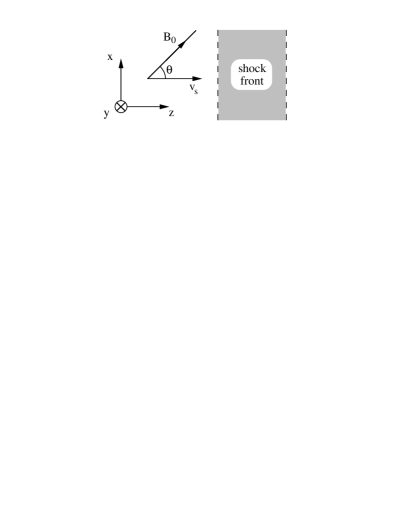
Figure 1: A sketch of the Cartesian reference frame used in this paper. In this frame the shock is at rest, and the unshocked material moves into the shock along the $z$-axis at speed $v_{s}$. The upstream magnetic field makes an angle $\theta$ to the incoming velocity, and lies in the $x$-$z$ plane, which is referred to in the text as the ‘shock plane’.

The continuity equations are

$$\rho v_{z}=\rho_{0}v_{s}$$ (1)

for the neutral fluid, and

$$\rho_{j}v_{jz}=\rho_{j0}v_{s}$$ (2)

for each of the charged species. The momentum equation for the neutral component of the fluid is:

$${d\over dz}\left(\rho v_{z}\mn@boldsymbol{v}\right)=\sum_{j}\gamma_{j}\rho_{j}\rho(\mn@boldsymbol{v}_{j}-\mn@boldsymbol{v})\,,$$ (3)

where $\gamma_{j}$ is related to the rate coefficient for elastic scattering between particles of species j and the neutrals, $<\sigma v>_{j}$, by

$$\gamma_{j}={<\sigma v>_{j}\over m_{j}+m}\,.$$ (4)

The drift of each charged species through the neutral gas is determined by a balance between electromagnetic forces and collisional drag (e.g. Shu 1983):

$$n_{j}Z_{j}e\left(\mn@boldsymbol{E}+{\mn@boldsymbol{v}_{j}\over c}\mn@boldsymbol{\times}\mn@boldsymbol{B}\right)+\gamma_{j}\rho_{j}\rho(\mn@boldsymbol{v}-\mn@boldsymbol{v}_{j})=0\,.$$ (5)

The inertia of the charged species has been neglected, which is valid provided that the time scale over which conditions change (i.e. the flow time through the shock front) is long compared to the collisional time with the neutrals. Equation (5) can be rewritten as

$$\mn@boldsymbol{v}_{j}=\mn@boldsymbol{v}+c\left(\beta_{j}\frac{(\mn@boldsymbol{B}\cdot\mn@boldsymbol{E}^{\prime})\mn@boldsymbol{B}}{B^{3}}\right.+\frac{\beta_{j}^{2}}{1+\beta_{j}^{2}}{\mn@boldsymbol{E}^{\prime}\mn@boldsymbol{\times}\mn@boldsymbol{B}\over B^{2}}+$$ (6)

$$\left.\frac{\beta_{j}}{1+\beta_{j}^{2}}\frac{\mn@boldsymbol{B}\mn@boldsymbol{\times}(\mn@boldsymbol{E}^{\prime}\mn@boldsymbol{\times}\mn@boldsymbol{B})}{B^{3}}\right)\,,$$

where

$$\mn@boldsymbol{E}^{\prime}=\mn@boldsymbol{E}+\mn@boldsymbol{v}\mn@boldsymbol{\times}\mn@boldsymbol{B}/c$$ (7)

is the electric field in the frame comoving with the neutrals, and $\beta_{j}$ is the Hall parameter for species j:

$$\beta_{j}={Z_{j}eB\over m_{j}c}\,{1\over\gamma_{j}\rho}\,,$$ (8)

i.e. the product of the gyrofrequency and the time scale for momentum exchange with the neutral fluid. Note that the sign of $\beta_{j}$ is determined by $Z_{j}$. The magnitude of the Hall parameters determines the magnetic flux transport in a weakly ionized medium (Draine 1980; Königl 1989). When $|\beta_{j}|\gg 1$, the electric and magnetic stresses individually dominate the drag force in equation (5) and must almost cancel, thus $\mn@boldsymbol{E}\approx-(\mn@boldsymbol{v}_{j}\times\mn@boldsymbol{B})/c$ and the particles are tied to the magnetic field lines. In the opposite limit, collisions with the neutrals decouple the charged particles from the magnetic field lines and $\mn@boldsymbol{v}_{j}\approx\mn@boldsymbol{v}$.

Rather than explicitly consider the drift velocity of each charged species, it is often more convenient to consider the expression for the current density

$$\mn@boldsymbol{J}=e\sum_{j}n_{j}Z_{j}\mn@boldsymbol{v}_{j}\$$ (9)

obtained by using (6) to substitute for $\mn@boldsymbol{v}_{j}$:

$$\mn@boldsymbol{J}=\sigma_{0}(\mn@boldsymbol{\hat{B}}\cdot\mn@boldsymbol{E}^{\prime})\mn@boldsymbol{\hat{B}}+\sigma_{1}\mn@boldsymbol{\hat{B}}\mn@boldsymbol{\times}\mn@boldsymbol{E}^{\prime}+\sigma_{2}(\mn@boldsymbol{\hat{B}}\mn@boldsymbol{\times}\mn@boldsymbol{E}^{\prime})\mn@boldsymbol{\times}\mn@boldsymbol{\hat{B}}\,,$$ (10)

where the components of the conductivity tensor are the conductivity parallel to the magnetic field,

$$\sigma_{0}=\frac{ec}{B}\sum_{j}n_{j}Z_{j}\beta_{j}\,,$$ (11)

the Hall conductivity,

$$\sigma_{1}=\frac{ec}{B}\sum_{j}\frac{n_{j}Z_{j}}{1+\beta_{j}^{2}}\,,$$ (12)

and the Pedersen conductivity

$$\sigma_{2}=\frac{ec}{B}\sum_{j}\frac{n_{j}Z_{j}\beta_{j}}{1+\beta_{j}^{2}}$$ (13)

(Cowling 1957; Nakano & Umebayashi 1986).

Now consider Maxwell’s equations. The induction equation yields $\nabla\mn@boldsymbol{\times}\mn@boldsymbol{E}=0$, implying that $E_{x}$ and $E_{y}$ are constant. Evaluating them far upstream gives:

$$E_{x}=0\,,$$ (14)

and

$$E_{y}=-{v_{s}\over c}B_{0x}\,.$$ (15)

Finally, $\nabla\cdot\mn@boldsymbol{B}=0$ implies that

$$B_{z}=B_{0z}\,.$$ (16)

Gauss’ law for the electric field is replaced by the condition for charge neutrality:

$$\sum_{j}Z_{j}n_{j}=0\,.$$ (17)

Ampere’s law reduces to

$${dB_{x}\over dz}={4\pi\over c}J_{y}\,,$$ (18)

$${dB_{y}\over dz}=-\,{4\pi\over c}J_{x}\,,$$ (19)

and

$$J_{z}=0\,.$$ (20)

Equation (20) is not independent as eqs (2) and (17) guarantee $J_{z}=0$ upon noting that $v_{jz}=v_{s}$ far upstream.

The derivatives in equation (3) can be eliminated using (5), (9), (16) and (18)–(20) to obtain expressions for the conservation of the $x$, $y$, and $z$ components of the total momentum flux:

$$\rho_{0}v_{s}v_{x}-{B_{x}B_{z}\over 4\pi}=-{B_{0x}B_{z}\over 4\pi}\,,$$ (21)

$$\rho_{0}v_{s}v_{y}-{B_{y}B_{z}\over 4\pi}=0\,,$$ (22)

and

$$\rho_{0}v_{s}v_{z}+{B_{x}^{2}+B_{y}^{2}\over 8\pi}=\rho_{0}v_{s}^{2}+{B_{0x}^{2}\over 8\pi}\,.$$ (23)

Thus we have a system of two ordinary differential equations in $B_{x}$ and $B_{y}$, (18) and (19), along with the algebraic relations (1), (2), (6), (9) (14)–(17), and (21)–(23).

2.2 Charged species

The pre-shock abundances of charged species are determined by a balance between cosmic-ray ionization and recombination occuring in the gas phase or on grain surfaces, and are therefore sensitive to the adopted grain model (Nishi et al. 1991).

When grains are of a single size $a\ga 0.1\mu$, recombination occurs primarily in the gas phase for ${n_{\rm H}}\la 10^{10}\,\mathrm{cm}^{-3}$, yielding a fractional ionization

$${n_{i}\over{n_{\rm H}}}\approx 10^{-8}\left({{n_{\rm H}}\over 10^{6}\,\mathrm{cm}^{-3}}\right)^{-1/2}$$ (24)

and an almost identical electron abundance (Elmegreen 1979; Nakano & Umebayashi 1986). The grains in the pre-shock gas carry a single negative charge, and assuming the the total mass of grains is 0.01 that of hydrogen, the grain abundance is $n_{g}/{n_{\rm H}}=2.5\times 10^{-14}$ for $a=0.4\mu$ (Draine et al. 1983), or $1.6\times 10^{-12}$ for $a=0.1\mu$. Under these conditions, the charging of the grains within the shock front proceeds by the sticking of electrons from the gas phase, and is limited by the Coulomb repulsion of incoming electrons by the grain. The resulting mean charge depends on the grain radius and the electron temperature (Draine 1980):

$$Z_{g}\approx{-4kT_{e}a\over e^{2}}\approx-4.8\left({T_{e}\over 200\,\mathrm{K}}\right)\left({a\over 10^{-5}\,\mathrm{cm}}\right)\,,$$ (25)

valid for $|Z_{g}|\gg 1$. The charges of individual grains fluctuate about the mean, but at any instant most are within 1 unit of the mean (Elmegreen 1979).

However, grains possess a power-law grain-size distribution (Mathis, Rumpl & Nordsieck 1978; Draine & Lee 1984),

$$\frac{dn}{da}=A{n_{\rm H}}a^{-3.5}$$ (26)

where $n_{(}a)$ is the number density of grains with radii smaller than $a$, $A=1.5\times 10^{-25}\,\mathrm{cm}^{-2.5}$, and the distribution runs from grain radii between lower and upper bounds $a_{1}=50$Å and $a_{2}=2500$Å. The lower bound is poorly constrained by observations, and the upper bound is uncertain in dense clouds, where grains are enlarged by icy mantles. In addition PAHs with $a\sim 3$Å and $n/{n_{\rm H}}\approx 2\times 10^{-7}$ (Léger & Puget 1984; Puget & Léger 1989), may be present, either as a distinct population or as the tail of an MRN distribution with $a_{1}\approx 3\AA$. For the sake of definiteness, I shall treat the PAHs as a distinct population. The MRN size distribution and the presence of PAHs increase the grain surface area and reduces the fractional ionization in the gas and the electron density by several orders of magnitude (Nishi et al. 1991; Kaufman & Neufeld 1996a). The electron density is comparable with, or less than, the density of grains and the charging of grains by electron sticking within the shock front is inhibited. Thus the grain charge remains at $Z_{g}=-1$, independent of $T_{e}$ in this case.

These two cases are considered here. First, for comparison with Pilipp & Hartquist (1994), I consider large grains of a single size. The charged species in this case are ions, electrons and negatively charged grains. The effect of an MRN grain-size distribution and PAHs are also considered. In this case the charged species are ions, electrons or PAHs, and negatively charged grains. The grains are still considered to be of a single size, but the grain size and abundance are chosen so that the contribution to the conductivity of the gas approximates that of the entire grain-size distribution (see §3.5).

I assume that the ions are singly charged and have mass $30m_{\rm H}$, as is typical for molecular or metal ions (e.g. HCO⁺, Mg⁺). Grains are taken to be spherical, all of the same radius $a$, with internal density $2.5\,\mathrm{g}\,\mathrm{cm}^{-3}$ and total mass 0.01 of the mass in hydrogen.

The rate coefficient for elastic scattering with the neutrals, $<\sigma v>_{j}$, depends in general on the fluid temperatures and the drift speed $|\mn@boldsymbol{v}_{j}-\mn@boldsymbol{v}|$. The scattering cross-section for ions has a $1/v$ dependence for ions with drift speeds below 20 $\,\mathrm{km\,s}^{-1}$, and the rate coefficient for ion-neutral scattering is constant, $<\sigma v>_{i}\approx 1.6\times 10^{-9}\,\mathrm{cm}^{3}\,\mathrm{s}^{-1}$, yielding a Hall parameter

$$\beta_{i}\approx 4600\left({B\over 1\,\mathrm{mG}}\right)\left({n_{\rm H}\over 10^{6}\,\mathrm{cm}^{-3}}\right)^{-1}$$ (27)

The PAHs have geometric cross-sections $\pi a^{2}\approx 3\times 10^{-16}(a/\mathrm{\AA})^{2}\,\mathrm{cm}^{-2}$, of order the polarization cross-section for elastic scattering from neutrals, $1.6\times 10^{-15}\times 10\,\mathrm{km\,s}^{-1}/|\mn@boldsymbol{v}_{g}-\mn@boldsymbol{v}|$. The PAHs are therefore treated as negatively charged ions, with $<\sigma v>_{\mathrm{PAH}}=<\sigma v>_{i}$, and $\beta_{\mathrm{PAH}}=-\beta_{i}$.

The elastic scattering cross-section for grains is the geometric cross-section, taken to be $\sigma_{g}=\pi a^{2}$, while for electrons, $\sigma_{e}\approx 1\times 10^{-15}\,\mathrm{cm}^{2}$ at energies below a few eV (Gilardini 1972). As $\sigma_{j}$ is energy-independent for both these species, the rate coefficient may be written as $\sigma_{j}u_{j}$ where the effective velocity is

$$u_{j}=\left[\frac{128}{9\pi}\left(\frac{kT}{m}+\frac{kT_{j}}{m_{j}}\right)+|\mn@boldsymbol{v}_{j}-\mn@boldsymbol{v}|^{2}\right]^{1/2}$$ (28)

(Draine 1986). The rate coefficient for electron scattering is determined by the electron thermal velocity, which is far in excess of both the electron-neutral drift speed and the neutral thermal velocity. The effective relative velocity between electrons and neutrals may therefore be written

$$u_{e}=\left(\frac{128kT_{e}}{9\pi m_{e}}\right)^{1/2}\,,$$ (29)

and the electron Hall parameter is

$$\beta_{e}\approx-2.5\times 10^{6}\left({B\over 1\,\mathrm{mG}}\right)\left({n_{\rm H}\over 10^{6}\,\mathrm{cm}^{-3}}\right)^{-1}\left(\frac{T_{e}}{200\,\mathrm{K}}\right)^{-1/2}$$ (30)

The grain thermal velocity is negligible compared with that for the neutrals, and

$$u_{g}=\left(\frac{128kT}{9\pi m}+|\mn@boldsymbol{v}_{g}-\mn@boldsymbol{v}|^{2}\right)^{1/2}\,.$$ (31)

The grain Hall parameter is then [eq. (35) of Draine (1980)]:

$$\beta_{g}\approx 0.22\,Z_{g}\left(\frac{B}{\,\mathrm{mG}}\right)\left(\frac{{n_{\rm H}}}{10^{6}\,\mathrm{cm}^{-3}}\right)^{-1}\left(\frac{a}{10^{-5}\,\mathrm{cm}}\right)^{-2}\times$$ (32)

$$\left(\frac{u_{g}}{\,\mathrm{km\,s}^{-1}}\right)^{-1}\,.$$

The rate coefficient for grain-neutral scattering depends on the neutral gas temperature and the grain-neutral drift speed. The grain charge and the electron scattering coefficients depend on the electron temperature. A calculation of the fluid temperatures is beyond the scope of the present work, so we assume that $u_{e}$, $u_{g}$ and $Z_{g}$ are constant throughout the flow, being fixed at values representative of conditions within the shock front. In particular, for the weak shock models ($v_{s}/v_{A}=1.5$) I adopt $T=100\,\mathrm{K}$, $T_{e}=200\,\mathrm{K}$, and $|\mn@boldsymbol{v}-\mn@boldsymbol{v}_{g}|=1\,\mathrm{km\,s}^{-1}$; and for the strong shock models ($v_{s}/v_{A}=10$), $T=1000\,\mathrm{K}$, $T_{e}=2000\,\mathrm{K}$, and $|\mn@boldsymbol{v}-\mn@boldsymbol{v}_{g}|=10\,\mathrm{km\,s}^{-1}$. The grain charge is either calculated from (25) using the adopted values of $T_{e}$ or is set to $-1$, depending on the chosen grain model.

3 Analysis

The shock structure is determined by the pair of differential equations (18) and (19) for $B_{x}$ and $B_{y}$ as a function of $z$, and the associated algebraic equations. There is no explicit reference to $z$, so given a choice of parameters, each shock solution can be represented as an integral curve in a phase space with coordinates $B_{x}$ and $B_{y}$, i.e. as a plot of $B_{y}(z)$ vs $B_{x}(z)$. This proves to be extremely useful in understanding the relationship between different shock solutions. Trajectories representing shock solutions begin and terminate at points representing upstream or downstream states, for which

$${d\over dz}\left(B_{x}\right)={d\over dz}\left(B_{y}\right)=0$$ (33)

(i.e. stationary points). The jump conditions, discussed in §3.1, show that there are three stationary points, all lying on the $B_{x}$ axis, which are denoted by U, F, and I in increasing order of $|B_{x}|$ (see Fig. 4). These points represent the upstream state, and possible downstream states corresponding to the fast and intermediate shocks respectively. The topology of the trajectories near the stationary points is obtained through a linear analysis in §3.2, where it is shown that U, F, and I are a source, saddle, and sink respectively. Thus it is not possible to find a fast shock trajectory by starting at the upstream state and integrating through the shock front towards the downstream state F; the trajectory should be integrated in the reverse direction from F to U.

To actually integrate equations (18) and (19), the $x$ and $y$ components of the current density ${\bf J}$ must be determined from the algebraic relations given $B_{x}$ and $B_{y}$ at some point in the shock front. The expressions for total momentum flux (21)–(23) allow $\mn@boldsymbol{v}$ to be expressed in terms of $\mn@boldsymbol{B}$, the neutral continuity equation then yields $\rho$, and the Hall parameters $\beta_{j}$ can then be calculated for each charged species. If $E^{\prime}_{z}$ were known then the charged particle drifts, and hence the current density, could be calculated from eq. (6). Actually $E^{\prime}_{z}$ is determined from the charge neutrality condition (17), by substituting the $z$-component of (6) and using (2) to relate $\rho_{j}$ and $v_{jz}$ (§3.3). The presence of $N$ charged species allows $N-1$ solutions for $E^{\prime}_{z}$ that yield drift velocities consistent with the charge neutrality condition at each point within the shock front. The choice of solution is dictated by requiring that the electric field vanish in the neutral rest frame ahead of (or behind) the shock front and be everywhere continuous.

Several regions of the phase space can be excluded on the grounds that the density of the neutrals, or of a charged species, becomes negative (§3.4). In particular, when $B^{2}$ becomes too large, the ram pressure must become negative (see eq [23]). The stationary point I becomes unphysical in this manner when the shock velocity is too large to allow intermediate shocks (see §3.1). When this is the case, there is also a locus in phase space where the ion and electron densities simultaneously diverge. However, it will turn out that the fast shock solutions avoid this locus.

The effect of an MRN grain-size distribution is examined in §3.5, where it is shown that it can be approximated by a single-size grain model with appropriately chosen ‘effective’ grain Hall parameters and abundances.

One interesting feature of the shock solutions is that within the shock front, the fluid motions and magnetic field are not restricted to lie in the plane containing the shock normal and the pre-shock magnetic field. The sense of motion out of the plane (i.e. ‘up’ or ‘down’) is determined by the asymmetry in the elastic scattering properties of species of different sign (i.e.$|\sigma_{1}|\neq 0$, see eq (12) ). Even if the Hall parameters of all charged species satisfy $|\beta_{j}|\la 1$, fast shocks remain coplanar if the properties of negatively and positively charged species are identical apart from the difference in sign. A criterion for this effect to be important is developed in §3.6. In essence, there should be ‘sufficient’ poorly-coupled charged particles, with the charge on the particles being preferentially of one sign.

Finally, in §3.6 I discuss the dimensionless parameters that determine the shock structure, and outline how the calculations presented in §4 were carried out.

3.1 Jump conditions

The boundary conditions for equations (18) and (19) are that the derivatives of $B_{x}$ and $B_{y}$ should vanish far away from the shock front. This implies that the current density, and hence (via eq [10]) the electric field in the rest frame of the neutrals also vanish at $z=\pm\infty$. In turn, (6) then guarantees that $\mn@boldsymbol{v}_{j}=\mn@boldsymbol{v}$ far upstream and downstream of the shock front. This is, of course, expected, and shows that the MHD jump conditions which relate the upstream and downstream states can be obtained by regarding the weakly ionized fluid as a plasma of density $\rho$ and velocity $\mn@boldsymbol{v}$, and equating the fluxes of mass and momentum of the combined fluid on either side of the front. The ionized component does not contribute significantly to the fluid density or mass flux, but does contribute to the momentum flux through the magnetic field (see eqs [21]–[23]). An energy condition is not required, as it is assumed that $T=0$.

In general, the MHD jump conditions imply that the pre-shock and post-shock magnetic fields and velocities are coplanar, and three broad classes of shocks can be distinguished on the basis of the behaviour of the field component transverse to the shock velocity, which either increases, decreases, or changes sign in going from upstream to downstream in fast, slow, and intermediate shocks respectively (e.g. Cowling 1976; Kennel et al. 1989).

The signal speeds in the fluid play a key role in determining the different kinds of shock the medium can support. The combined fluid supports fast, intermediate and slow waves with signal speeds for propagation in the direction normal to the shock front of

$$v_{\mathrm{fast}}=\left({B^{2}\over 4\pi\rho}\right)^{1/2}=v_{A}$$ (34)

where $v_{A}$ is the Alfvén speed,

$$v_{\mathrm{int}}=\left({B_{z}^{2}\over 4\pi\rho}\right)^{1/2}=v_{A}\cos\theta\,,$$ (35)

and

$$v_{\mathrm{slow}}=0\,,$$ (36)

respectively. The assumption that the plasma is cold eliminates shock transitions that have downstream velocities below the slow speed (i.e. slow shocks and three classes of intermediate shock, see Kennel et al. 1989).

Far away from the shock front,

$$\mn@boldsymbol{E}={-\mn@boldsymbol{v}/c}\mn@boldsymbol{\times}\mn@boldsymbol{B}$$ (37)

which implies that

$$v_{y}B_{z}-v_{z}B_{y}=0\,,$$ (38)

and

$$v_{z}B_{x}-v_{x}B_{z}=v_{s}B_{0x}\,.$$ (39)

Equations (1) and (21)–(23) for mass and momentum flux conservation also hold and combined with (38) and (39) yield a complete set of jump conditions.

Equations (22) and (38) both express $v_{y}$ downstream in terms of $B_{y}$, implying that either $B_{y}=0$, or that

$$v_{z}={B_{z}^{2}\over 4\pi\rho_{0}v_{s}}\,.$$ (40)

In the latter case, the $z$-components of the pre-shock and post-shock velocities are equal to the intermediate speed, and the transverse components of the magnetic field and fluid velocity change direction in such a way as to conserve the transverse momentum flux. There is no compression or entropy increase across such a transition, which exists in ideal MHD as a ‘rotational discontinuity’ (e.g. Cowling 1976). In the non-ideal case it is unsteady, broadening diffusively with time (Wu 1988b), and we shall not discuss it further here.

Thus we set $B_{y}=0$ and $v_{y}=0$ and use (21) and (23) to eliminate $v_{x}$ and $v_{z}$ in favour of $B_{x}$ in (39), to obtain a cubic in $B_{x}$ whose solutions satisfy the jump conditions. The upstream state is a solution, so $(B_{x}-B_{0x})$ factors out of the cubic to yield a quadratic

$$B_{x}^{2}+B_{0x}B_{x}+2\left(B_{z}^{2}-4\pi\rho_{0}v_{s}^{2}\right)=0\,$$ (41)

with positive and negative roots that are candidate downstream states for fast and intermediate shock transitions respectively.

The roots correspond to physically acceptable downstream states if there is compression across the shock front, i.e. for $0<v_{z}<v_{s}$. From eq (23), the condition on $B_{x}$ is:

$$1<\left({B_{x}\over B_{0x}}\right)^{2}<1+{8\pi\rho_{0}v_{s}^{2}\over B_{0x}^{2}}\,.$$ (42)

When $v_{s}/v_{A}>1$, the positive root yields a fast shock, and when $\cos\theta<v_{s}/v_{A}<{\sqrt{2}}\,\cot\theta$ the negative root yields an intermediate shock (c.f. Kennel et al. 1989). The regime in which intermediate shocks are allowed is sketched in Fig. 2.

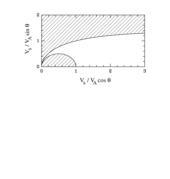
Figure 2: A polar plot of the conditions for the existence of intermediate shocks. A point on the plane represents a shock velocity, with polar radius representing the shock speed $v_{s}$, and polar angle representing the angle $\theta$ between the pre-shock magnetic field and the shock normal. Intermediate shocks do not exist in the shaded region.

3.2 Classification of the stationary points

The stationary points can be classified as source, sink or saddle by linearizing the equations for shock structure around each point. I use eqs. (1) and (16)–(18) for the conservation of neutral mass flux and total momentum flux, but rather than explicitly considering the drift velocities of the charged species given by (6), it is more convenient to use (10). Since $\mn@boldsymbol{E}^{\prime}=0$ outside the shock front, the linearised version of this equation is

$$\delta\mn@boldsymbol{J}=\sigma_{0}(\mn@boldsymbol{\hat{B}}\cdot\delta\mn@boldsymbol{E}^{\prime})\mn@boldsymbol{\hat{B}}+\sigma_{1}\mn@boldsymbol{\hat{B}}\mn@boldsymbol{\times}\delta\mn@boldsymbol{E}^{\prime}+\sigma_{2}(\mn@boldsymbol{\hat{B}}\mn@boldsymbol{\times}\delta\mn@boldsymbol{E}^{\prime})\mn@boldsymbol{\times}\mn@boldsymbol{\hat{B}}$$ (43)

Assuming that the perturbations are steady, independent of $x$ and $y$, and vary exponentially in $z$ as $e^{\lambda z}$, the resulting dispersion relation is

$$\left[(v_{s}^{2}-v_{A}^{2}\cos^{2}\theta)\mu-\frac{(\sigma_{1}^{2}+\sigma_{2}^{2})\sin^{2}\theta+\sigma_{0}\sigma_{2}\cos^{2}\theta}{\sigma_{0}}\right]\times$$

$$\qquad\left[(v_{s}^{2}-v_{A}^{2})\mu-\sigma_{2}\right]+\sigma_{1}^{2}\cos^{2}\theta=0\,,$$ (44)

where

$$\mu=\frac{4\pi v_{A}(\sigma_{1}^{2}+\sigma_{2}^{2})}{c^{2}v_{s}^{2}\lambda}\,.$$ (45)

The nature of the stationary point is determined by the sign of the real part of $\lambda$, which is the same as that of $\mu$. Noting that $\sigma_{0}$, $\sigma_{2}>0$, and using $v_{s}>v_{A}$, we find that the real parts of the roots of the dispersion relation are positive, so the upstream state is a source.

The dispersion relation can be applied to the downstream states F and I by noting that a boost from the shock frame to a frame in which the shock is stationary and the downstream fluid velocity is normal to the shock does not affect the assumptions of steady state and the $e^{\lambda z}$ dependence of the perturbations. Thus (44) can be applied downstream on replacing $v_{s}$ by $v_{z}$, $v_{A}$ by the downstream Alfvén speed, and $\theta$ by the value of $\cos^{-1}(B_{x}/B)$ far downstream. Re-evaluating the dispersion relation at F (for which $v_{A}>v_{z}>v_{A}\,{\rm cos}\,\theta$) shows that the roots there are real and of opposite signs, and at I (where $v_{z}<v_{A}\,{\rm cos}\,\theta$) the roots have negative real part. Thus F is a saddle point, and I is a sink.

Finally, we note that at U and I, when

$$(v_{z}^{2}-v_{A}^{2})\frac{\sigma_{1}^{2}+\sigma_{2}^{2}}{\sigma_{0}^{2}}-v_{z}^{2}\frac{\sigma_{2}}{\sigma_{0}}$$

$$+2(v_{z}^{2}-v_{A}^{2})^{1/2}(v_{z}^{2}-v_{A}^{2}\cos^{2}\theta)^{1/2}\frac{\cos\theta}{\sin^{2}\theta}\frac{|\sigma_{1}|}{\sigma_{0}}>0\,$$ (46)

the roots of the dispersion relation, eq. (44) are complex conjugates and trajectories spiral out of U and into I. Typically, $\sigma_{0}^{2}\gg\sigma_{1}^{2}+\sigma_{2}^{2}$ and $v^{2}\gg v_{A}^{2}$, and the criterion becomes

$$|\sigma_{1}|>\frac{\cos\theta}{\sin^{2}\theta}\sigma_{2}\,,$$ (47)

or $|\beta_{g}|\la 0.3$ for $\theta=30\degr$.

3.3 The charge neutrality condition

To actually integrate equations (18) and (19), the $x$ and $y$ components of the current density ${\bf J}$ must be determined given $B_{x}$ and $B_{y}$. This is achieved as follows. The expressions for total momentum flux (21)–(23) allow $\mn@boldsymbol{v}$ to be expressed in terms of $\mn@boldsymbol{B}$, the continuity equation then yields $\rho$, and thus the Hall parameters $\beta_{j}$ can be calculated for each charged species. At this point, $E^{\prime}_{x}$ and $E^{\prime}_{y}$ can be found from (7), (14) and (15), so that if $E^{\prime}_{z}$ (or equivalently $E_{z}$) were known then the charged particle drifts, and hence the current density, could be calculated from eq. (6). Actually $E^{\prime}_{z}$ is determined by the charge neutrality condition (17), by substituting the $z$-component of (6) and using (2) to relate $\rho_{j}$ and $v_{jz}$:

$$0=\sum_{j}\frac{n_{j0}Z_{j}}{v_{jz}}\,.$$ (48)

Noting that eq. (6) implies that $v_{jz}$ can be written in the form

$$v_{jz}=n_{j0}Z_{j}(p_{j}E^{\prime}_{z}+q_{j})$$ (49)

where

$$p_{j}=\frac{1}{n_{j0}Z_{j}}\frac{\beta_{j}(1+\beta_{j}^{2}B_{z}^{2}/B^{2})}{(1+\beta_{j}^{2})}$$ (50)

and

$$q_{j}=\frac{1}{n_{j0}Z_{j}v_{s}}\left[v_{z}+\frac{c\beta_{j}^{2}}{1+\beta_{j}^{2}}\frac{(\mn@boldsymbol{E}^{\prime}\mn@boldsymbol{\times}\mn@boldsymbol{B})_{z}}{B^{2}}+\right.$$ (51)

$$\qquad\qquad\left.\frac{c\beta_{j}^{3}}{1+\beta_{j}^{2}}\frac{(\mn@boldsymbol{B}\mn@boldsymbol{\cdot}\mn@boldsymbol{E}^{\prime})B_{z}}{B^{3}}\right]\,,$$

eq. (48) can be recast as

$$\sum_{j}\frac{1}{p_{j}E^{\prime}_{z}+q_{j}}=0\,.$$ (52)

In this expression, $p_{j}$ and $q_{j}$ are known quantities, and the task is to determine $E^{\prime}_{z}$. If N is the number of charged species, the sum regarded as a function of $E^{\prime}_{z}$ has N poles at $E^{\prime}_{z}=E_{j}$ where $E_{j}=-q_{j}/p_{j}$. If the poles are ordered so that $E_{1}<E_{2}\ldots<E_{n}$, then there is a zero between each pair $E_{j}$, $E_{j-1}$. Thus locally there are several values of $E^{\prime}_{z}$ which will produce particle drifts with no net current. The correct choice is dictated by the requirement that $E^{\prime}_{z}(z)$ be smooth and go to zero ahead of and behind the shock.

Multiplying (52) by $\prod_{j}(p_{j}E^{\prime}_{z}+q_{j})$ yields a polynomial in $E^{\prime}_{z}$ which for N charged species has N-1 solutions. For the case $N=3$ relevant to this paper, eq. (52) yields a quadratic in $E^{\prime}_{z}$:

$$a_{2}{E^{\prime}_{z}}^{2}+a_{1}E^{\prime}_{z}+a_{0}=0\,,$$ (53)

where the required root is

$$E^{\prime}_{z}=\frac{-a_{1}-\sqrt{a_{1}^{2}-4a_{0}a_{2}}}{2a_{2}}\,.$$ (54)

3.4 Forbidden regions of phase space

Several regions in the $B_{x}$–$B_{y}$ phase space are forbidden in the sense that the density of one or more species formally becomes negative.

Firstly, the magnetic field strength is limited by :

$$\frac{B_{x}^{2}+B_{y}^{2}}{B_{0}^{2}}<\frac{2v_{s}^{2}}{v_{A}^{2}}+\sin^{2}\theta\,$$ (55)

otherwise eq (23) implies that $v_{z}$ would need to be negative to conserve the total z-momentum flux. As the magnetic field approaches the limiting value, $v_{z}$ tends to zero and the neutral density diverges.

An additional restriction is imposed by requiring that $v_{jz}>0$ for each charged species. The locus $v_{jz}=0$ corresponds to diverging particle density (see eq. [2]), and the charge neutrality requirement forces the density of an oppositely charged species to also diverge there. Thus for the system of ions, electrons, and negatively charged grains considered here, there are two loci: $v_{iz}=v_{ez}=0$, and $v_{iz}=v_{gz}=0$. Which of these loci is relevant is intimately related to the choice of $E^{\prime}_{z}$ as determined by the charge neutrality condition. As the ions and electrons are better tied to the field lines than the grains, the choice of $E^{\prime}_{z}$ shows that it is the first condition that is relevant. For $|\beta_{e}|$ and $\beta_{i}\gg 1$, the locus $v_{iz}=v_{ez}=0$ is given by

$$\left(\frac{B_{x}}{B_{0}}+\frac{v_{s}^{2}-v_{\mathrm{int}}^{2}}{v_{\mathrm{int}}^{2}}\sin\theta\right)^{2}+\left(\frac{B_{y}}{B_{0}}\right)^{2}=$$

$$=\frac{v_{s}^{4}}{v_{\mathrm{int}}^{4}}\left(\sin^{2}\theta-2\frac{v_{\mathrm{int}}^{2}}{v_{s}^{2}}\right)\,,$$ (56)

a circle centred on a point on the negative $B_{x}$ axis. The region enclosed within the locus is unphysical, as the electron and ion densities become negative there. This locus exists only if the right-hand side of eq. (56) is positive, i.e. when $v_{s}>\sqrt{2}v_{A}\mathrm{cot}\,\theta$. This is precisely the criterion for the non-existence of the intermediate shocks, so the unphysical region in the $B_{x}$–$B_{y}$ plane is only relevant for fast shock waves.

The constraint that $v_{jz}>0$ arises from the continuity equations for the charged species and the requirement that the charged particle densities should remain positive. To some degree this is an artifact of the neglect of ionization and recombination processes ocurring within the shock front, recombinations serving to limit the divergence of the charged particle densities. In principle, charged particles could drift backwards at some point within the shock, with a steady state being maintained by recombinations around the points where $v_{jz}=0$. In any case, the increase in charged particle density increases the currents that can flow within the shock front and prevent the trajectories from crossing into the unphysical zone (see §4.2).

3.5 The grain-size distribution

The majority of studies (e.g. Draine et al. 1983; Pilipp & Hartquist 1994) assumed grain sizes of 0.4 $\mu$ and 0.1 $\mu$ respectively. However, the smaller grains in an MRN distribution dominate the conductivity of the gas (Nakano & Umebayashi 1986) and determine the shock structure (Kaufman & Neufeld 1996a). If all grains have the same drift velocity, the cross-section for collisions with neutrals scales with grain radius as $a^{2}$, and the differential contribution to the drag by grains with radii in the range $a$ to $a+da$ scales as $a^{-1.5}da\propto da^{-0.5}$. (The decrease at larger radii will be a little steeper as grains become more strongly tied to the neutral gas.) The dust contribution to the drag force on the neutral gas is therefore dominated by the smallest grains, but a broad range of sizes contributes significantly to the total drag force.

In principle, the equations of §2.1 can be applied in this case with each size grain treated as a different species, and the sums over $j$ converted to integrals over grain size. Such a treatment is complicated by the dependence of $|\mn@boldsymbol{v}_{g}-\mn@boldsymbol{v}|$ on grain size, and lies beyond the scope of the present paper. Instead, I develop an approximate treatment in which an effective grain size and number density are determined.

The rationale for selecting the ‘effective’ pre-shock grain no. density $n_{g}$ and Hall parameter $\beta_{g}$ is that the grain contribution to the components of the conductivity tensor perpendicular to $\mn@boldsymbol{B}$, i.e. $\sigma_{1}$ and $\sigma_{2}$, should match that for the entire size distribution. It is not possible to simultaneously match the contribution to the conductivity parallel to the magnetic field,$\sigma_{0}$, but this is dominated in any case by the species that have large Hall parameters, i.e. ions, and electrons or PAHs (see [11]). Thus $n_{g}$ and $\beta_{g}$ must satisfy

$$\frac{n_{g}}{1+\beta_{g}^{2}}=\int_{a_{1}}^{a_{2}}\frac{dn_{g}/da}{1+\beta_{g}^{2}}\,da=NI_{1}$$ (57)

and

$$\frac{n_{g}|\beta_{g}|}{1+\beta_{g}^{2}}=\int_{a_{1}}^{a_{2}}\frac{|\beta_{g}|\,dn_{g}/da}{1+\beta_{g}^{2}}\,da=NI_{2}$$ (58)

where

$$N={\textstyle\frac{2}{5}}A{n_{\rm H}}a_{1}^{-2.5}\approx 3.4\times 10^{-10}{n_{\rm H}}\left(\frac{a_{1}}{50\mathrm{\AA}}\right)^{-2.5}$$ (59)

is the total number of grains with radii between $a_{1}$ and $a_{2}$ apart from a negligible correction factor of $[1-(a_{1}/a_{2})^{2.5}]$,

$$I_{1}={\textstyle\frac{5}{4}}\beta_{1}^{-5/4}\int_{\beta_{2}}^{\beta_{1}}\frac{\beta^{1/4}}{1+\beta^{2}}\,d\beta\,,$$ (60)

and

$$I_{2}={\textstyle\frac{5}{4}}\beta_{1}^{-5/4}\int_{\beta_{2}}^{\beta_{1}}\frac{\beta^{5/4}}{1+\beta^{2}}\,d\beta\,,$$ (61)

where $\beta_{1}$ and $\beta_{2}$ are the absolute values of the Hall parameters for grains of sizes $a_{1}$ and $a_{2}$ respectively. The integrals over $a$ have been converted to integrals over $\beta\propto a^{-2}$. Thus

$$\beta_{g}=-I_{2}/I_{1}$$ (62)

and

$$n_{g}=(1+\beta_{g}^{2})I_{1}N\,.$$ (63)

The integrals for $I_{1}$ and $I_{2}$ are solved analytically below, but it is instructive to derive approximate values before presenting the exact results. These can be obtained by setting $1+\beta^{2}$ in (60) and (61) to 1 for $\beta<1$ and to $\beta^{2}$ for $\beta>1$. This yields

$$I_{1}\approx\left\{\begin{array}[]{ll}1&\beta_{2}\ll\beta_{1}\ll 1\\[3.0pt] {\textstyle\frac{4}{3}}\beta_{1}^{-5/4}&\beta_{2}\ll 1\ll\beta_{1}\\[3.0pt] {\textstyle\frac{5}{3}}(a_{2}/a_{1})^{3/2}\beta_{1}^{-2}&1\ll\beta_{2}\ll\beta_{1}\end{array}\right.$$ (64)

and

$$I_{2}\approx\left\{\begin{array}[]{ll}{\textstyle\frac{5}{9}}\beta_{1}&\beta_{2}\ll\beta_{1}\ll 1\\[3.0pt] 5\beta_{1}^{-1}&1\ll\beta_{1}\\[3.0pt] \end{array}\right.$$ (65)

The approximation is poor for $I_{1}$ when $\beta_{2}\ll 1\ll\beta_{1}$, as there is a significant contribution for $\beta$ near 1. Thus the expression given above includes a correction factor of $1/2$. These expressions yield estimates of the effective grain parameters:

$$\frac{|\beta_{g}|}{\beta_{1}}\approx\left\{\begin{array}[]{ll}{\textstyle\frac{5}{9}}&\beta_{2}\ll\beta_{1}\ll 1\\[3.0pt] {\textstyle\frac{3}{2}}\beta_{1}^{-3/4}&\beta_{2}\ll 1\ll\beta_{1}\\[3.0pt] 3(a_{2}/a_{1})^{-3/2}&1\ll\beta_{2}\ll\beta_{1}\,,\end{array}\right.$$ (66)

and

$$\frac{n_{g}}{N}\approx\left\{\begin{array}[]{ll}1&\beta_{2}\ll\beta_{1}\ll 1\\[3.0pt] 3\beta_{1}^{-3/2}&\beta_{2}\ll 1\ll\beta_{1}\\[3.0pt] 15(a_{2}/a_{1})^{-3/2}&1\ll\beta_{2}\ll\beta_{1}\,.\end{array}\right.$$ (67)

These approximations show that when all of the grains are decoupled from the magnetic field ($\beta_{1}\ll 1$), the effective Hall parameter is roughly half that of the most strongly coupled grains, and all of the grains contribute to the noncoplanarity. When all of the grains are coupled ($\beta_{2}\gg 1$), $\beta_{g}\approx 3(a_{2}/a_{1})^{1/2}\beta_{2}$, and the number of participating grains is of order one per cent. However, the most relevant case is the intermediate regime, in which the smallest grains are coupled to the field, whereas the largest grains are not ($\beta_{2}\ll 1\ll\beta_{1}$), as from (32),

$$\beta_{1}\approx 8.6\left(\frac{B/\,\mathrm{mG}}{{n_{\rm H}}/10^{6}\,\mathrm{cm}^{-3}}\right)\left(a\over{50\AA}\right)^{-2}\\ \left(\frac{v_{\mathrm{eff}}}{10\,\mathrm{km\,s}^{-1}}\right)^{-1}\,,$$

and $\beta_{2}\approx 2500\beta_{1}$. Then the effective Hall parameter is of order unity, and a tenth of the grains or more can be regarded as participating.

$I_{1}$ and $I_{2}$ can be found analytically by making the substitution $x=\beta^{1/4}$ and using the identity

$$I_{m,n}(x)\equiv\int\frac{x^{m-1}}{1+x^{2n}}\,dx=$$ (68)

$$\sum_{k=1}^{n}\left[\sin m\theta_{k}\tan^{-1}\left(\frac{x-\cos\theta_{k}}{\sin\theta_{k}}\right)-\right.$$

$$\left.\frac{1}{2}\cos m\theta_{k}\ln(1-2x\cos\theta_{k}+x^{2})\right]\,,$$

where

$$\theta_{k}=\frac{2k-1}{2n}\pi\,,$$ (69)

which is valid for $m$ and $n$ natural numbers and $m<2n$ (Gradshteyn & Ryzhik 1965, 2.146). Then

$$I_{1}=5\beta_{1}^{-5/4}\left[I_{5,4}(\beta_{1}^{1/4})-I_{5,4}(\beta_{2}^{1/4})\right]$$ (70)

$$I_{2}=5\beta_{1}^{-5/4}\left[I_{1,4}(\beta_{2}^{1/4})-I_{1,4}(\beta_{1}^{1/4})+\beta_{1}^{1/4}-\beta_{2}^{1/4}\right]$$ (71)

Figure 3: The effective single-size grain parameters corresponding to an MRN distribution between 50 and 2500 Å, plotted as a function of the magnitude of the Hall parameter of the 50 Å grains, $\beta_{1}$. The solid curve shows the effective grain no. density relative to the total grain no. density, and the dashed curve shows the effective Hall parameter $\beta_{g}$ relative to $\beta_{1}$. $\beta_{1}$ is typically in the range 0.1 to 1 in dense clouds.

The corresponding values of $n_{g}$ and $\beta_{g}$ are plotted in Figure 3. As $\beta_{1}$ ranges from 1 to 10, $n_{g}/N$ decreases from about 1 to 0.5, and $|\beta_{g}|$ increases from 0.6 to 3. Thus the effective Hall parameter typically lies between 0.1 and 2, and the effective number density is between 0.5 and 1 of the actual charged grain number density.

3.6 Criteria for non-coplanarity of fast shocks

The general criterion is simply $|\sigma_{1}|\ga\sigma_{2}$. A rough criterion, assuming that ions and electrons are well-coupled is that the contribution of poorly-coupled grains to the current is a significant fraction of the current that would flow within the shock in the absence of grains. The former can be estimated by assuming that the grain-ion drift is $1/2$ of the shock speed, the latter from the magnetic field gradient in a perpendicular C-type shock, yielding:

$${\scriptstyle\frac{1}{2}}n_{g}e|Z_{g}|v_{s}\ga\frac{c}{4\pi}\frac{\sqrt{2}v_{s}/v_{A}B_{0}}{L_{\mathrm{shock}}}$$ (72)

where

$$L_{\mathrm{shock}}=\frac{\sqrt{2}v_{A}}{n_{i}<\sigma v>_{i}}$$ (73)

is the characteristic shock thickness in the absence of grains (Wardle 1990). This criterion can be rearranged to yield:

$$\frac{n_{g}|Z_{g}|}{n_{i}}\beta_{i}\ga 1\,.$$ (74)

A more rigorous derivation begins by considering the grain contribution to the net drag force on the neutrals, or equivalently, the Lorentz force per unit volume:

$$\frac{\mn@boldsymbol{J}\mn@boldsymbol{\times}\mn@boldsymbol{B}}{c}=\frac{\sigma_{1}(\mn@boldsymbol{B}\mn@boldsymbol{\times}\mn@boldsymbol{E}^{\prime})\mn@boldsymbol{\times}\mn@boldsymbol{\hat{B}}+\sigma_{2}\mn@boldsymbol{B}\mn@boldsymbol{\times}\mn@boldsymbol{E}^{\prime}}{c}\,.$$ (75)

Assuming that $n_{g}\ll n_{e}\approx n_{i}$, and that $|\beta_{e}|\gg\beta_{i}\gg 1$, then the electron contribution is dominated by the ions, and the ion contribution to eq. (75) is

$$\left(\frac{\mn@boldsymbol{J}\mn@boldsymbol{\times}\mn@boldsymbol{B}}{ec}\right)_{\mathrm{i}}\approx\frac{n_{i}Z_{i}}{\beta_{i}}\,{\mn@boldsymbol{B}\mn@boldsymbol{\times}\mn@boldsymbol{E}^{\prime}}\,.$$ (76)

The grains contribute a force

$$\left(\frac{\mn@boldsymbol{J}\mn@boldsymbol{\times}\mn@boldsymbol{B}}{ec}\right)_{\mathrm{g}}\approx\frac{n_{g}|Z_{g}|}{1+\beta_{g}^{2}}\,(\mn@boldsymbol{\hat{B}}\mn@boldsymbol{\times}\mn@boldsymbol{E}^{\prime})\mn@boldsymbol{\times}\mn@boldsymbol{B}+\frac{n_{g}Z_{g}\beta_{g}}{1+\beta_{g}^{2}}\,\mn@boldsymbol{B}\mn@boldsymbol{\times}\mn@boldsymbol{E}^{\prime}$$ (77)

which dominates the ion drag provided that

$$\frac{|n_{g}Z_{g}|}{\sqrt{1+\beta_{g}^{2}}}\ga\frac{n_{i}Z_{i}}{\beta_{i}}\,.$$ (78)

The grain contribution is non-coplanar when $\beta_{g}\la 1$, thus combining this requirement with (78) yields (74).

The criterion for non-coplanarity, eq. (75), is the opposite to that given by Pilipp & Hartquist (1994, §3). Their sense of the criterion implies significant rotation in the limit of no grains, $n_{g}\rightarrow 0$, yet fast shock waves in this limit are planar. This was based upon a linear analysis of the shock precursor, and derived for the growing mode that is relevant to intermediate shock precursors, rather than the fast shocks which the criterion of eq. (75) addresses. Even when the Hall current vanishes – in the pure ambipolar diffusion limit – rotation in intermediate shock precursors is enforced by the requirement imposed by the jump conditions that the sign of $B_{x}$ changes across the shock front. Fast shocks, however, will not exhibit rotation unless the Hall current is important.

3.7 Numerical solution

The equations are put in dimensionless form by using $v_{s}$, $B_{0}$, $v_{s}B_{0}/c$ as units of velocity, magnetic field strength and electric field respectively. The parameters that appear in the equations are

1. $A=v_{s}/v_{A}$, the Alfvén number, which determines the strength of the shock,

2. $\theta$, the angle between the upstream magnetic field and the shock velocity,

3. $\beta_{j0}$, the Hall parameters in the pre-shock gas (eq. [8]), which determine whether the field is frozen into each species ($\beta_{j}\ga 1$), and

4. $\gamma_{j}\rho_{j0}/\sum_{j}\gamma_{j}\rho_{j0}$, which is a relative measure of the contribution of species $j$ to the net drag force on the neutral component given equal drift velocities of the charged species.

The overall normalisation of the drag forces appears in the expression for a characteristic length scale,

$$L_{s}={v_{A}/\sum_{j}\gamma_{j}\rho_{j0}}\,,$$ (79)

which appears as the unit of length in the dimensionless equations for $dB_{x}/dz$ and $dB_{y}/dz$. Although this is approximately equal to the shock thickness $L_{\mathrm{shock}}$ when the charged species are well coupled (Wardle 1990, see also Smith 1992), it overestimates the thickness in the present case, when the grains do not drift with the magnetic field.

Numerical integration of the differential equations forwards (backwards) in $z$ from the upstream (downstream) state yield the shock structure, i.e $B_{x}$ and $B_{y}$ (and hence velocity components and fluid densities), as a function of $z$. The derivatives of $B_{x}$ and $B_{y}$ vanish far upstream and downstream (in the limit that $|z|\rightarrow\infty$), so the field components have to be perturbed before commencing the integration. Because the Hall parameters are extremely large for the ions and electrons ($\approx 10^{4}$, and $10^{6}$ respectively) the equations are stiff (this could be removed by assuming that the ions and electrons are well-tied to the field lines), so I use the integration method of Gear (1971).

4 Results

In this section, I present solutions for C-type shock waves propagating into dense molecular gas. Initially, a single-size grain model is adopted, with grain radius 0.4 $\mu$ and abundance $n_{g}/{n_{\rm H}}=2.5\times 10^{-14}$. The pre-shock density is set to ${n_{\rm H}}=10^{6}\,\mathrm{cm}^{-3}$, $B_{0}=1$ mG, and $\theta=30\degr$, and the pre-shock ion density is $n_{i}/{n_{\rm H}}=10^{-8}$.

Mildly super-Alfvénic shocks with $v_{s}/v_{A}=1.5$ are considered in §4.1. There is a family of intermediate shocks and a single fast shock solution at this shock speed. Stronger shocks, with ($v_{s}/v_{A}=10$), for which only the fast shock solution exists, are considered in §4.2. For the chosen parameters, the fast shock is significantly non-coplanar. The effect of adopting a grain size of 0.1 $\mu$, with a larger grain abundance, and of increasing the pre-shock density to $10^{7}\,\mathrm{cm}^{-3}$ are also examined.

Finally, the dynamical effects of an MRN grain-size distribution are examined in §4.3, where solutions are presented for cases with and without PAHs present.

4.1 Weak fast and intermediate shocks

For these solutions we adopt 100 and 200 K as the effective values of neutral and electron temperatures respectively, consistent with the results of Pilipp & Hartquist (1994), and the effective grain-neutral drift speed is set at 1 $\,\mathrm{km\,s}^{-1}$. With these choices, the mean grain charge $Z_{g}=-19.15$, and the ion, electron and grain Hall parameters in the pre-shock gas are 4600, $-2.503\times 10^{6}$, and $-0.1606$ respectively.

Figure 4: The phase space for shocks with $v_{s}/v_{A}=1.5$ and $\theta=30\degr$. Each shock solution is represented by a trajectory $(B_{x}(z),B_{y}(z))$. The point U indicates the upstream state, and the points F and I indicate the downstream states for fast and intermediate shocks respectively. The solid curve running from U to F is the trajectory for the fast shock solution, and the two solid curves running from F to I are intermediate shocks that can exist in the downstream state of the fast shock. The remaining trajectories (dotted and dashed lines) are a one-parameter family of intermediate shock waves. The structure of the three intermediate shock solutions indicated by dashed trajectories are plotted in Figures 5, 6 and 7.

Both intermediate and fast shocks exist for these parameters, with $B_{x}/B_{0}$ equal to 0.5 for the upstream state, and 1.5 and $-2.0$ for the downstream states of fast and intermediate shocks respectively. Before considering the structure of individual shock waves it is instructive to examine the entire set of shock transitions in the $B_{x}$–$B_{y}$ phase space (see §2.3). This is presented in Figure 4, with points marked on the $B_{x}$ axis corresponding to the upstream state (U) and to the downstream states for fast (F) and intermediate shocks (I). Only integral curves corresponding to shock solutions, i.e. beginning and ending at stationary points, are plotted .

The one-parameter family of solutions running from U to I are intermediate shocks, in which $\mn@boldsymbol{B}_{\perp}$ rotates by 180° through the shock front. A unique solution, the fast shock, runs from U to F close to the $B_{x}$ axis. In addition, two intermediate shocks run from F to I with opposite senses of transverse field rotation. There are no other acceptable solutions, as the remaining curve terminating at F, and the remaining set of curves terminating at I are physically unacceptable, with $\mn@boldsymbol{B}$ diverging at $z=-\infty$.

The slight asymmetry between the half-planes $B_{y}>0$ and $B_{y}<0$ reflects the asymmetry in the properties of charged particles of different sign, namely that the negatively-charged grains are partially decoupled from the magnetic field, whereas the remaining charged species are well coupled. If all charged species were well coupled, the diagram would be symmetric upon reflection about the $B_{x}$ axis.

Figure 5: The structure of the intermediate shock corresponding to the dashed trajectory leaving the point U in figure 4 towards the upper half-plane of phase space. The top panel shows the transverse velocity components of the neutrals (solid), ions and electrons (dashed), and grains (dotted). The $z$-component of velocity is plotted in the middle panel, and the transverse magnetic field components are plotted in the lower panel.

Figure 6: As for Figure 5, but for the intermediate shock whose dashed trajectory leaves U in Figure 4 towards the lower half-plane of the phase space.

Figure 5 and 6 show the detailed structure of two of the intermediate shocks whose trajectories in Fig. 4 are indicated by dashed lines. The rotation of $\mn@boldsymbol{B}_{\perp}$ has the opposite sense in each shock. The shocks are similar to those presented by Pilipp & Hartquist (1994) (see their Figs 1a^′ –1c^′ and 2a^′), with $B_{x}$ changing sign across the shock front, and the $y$-components of velocity and magnetic field becoming comparable to the $x$-component within the shock front. The difference between the shock structures lies primarily in the signs of the $y$-components. This would be the only difference if all of the charged species were tied to the field lines, when the phase space is symmetric under reflection in the $x$-axis. However, as the grains are poorly coupled to the magnetic field the grain drift through the neutrals is much smaller than that of the ions, electrons and magnetic field, and the direction of this drift shows distinct differences between the two shocks. For example, the grains are declerated before the neutrals in the middle panel of Fig. 5, and lag the neutrals in the middle panel of Fig. 6. Similar differences exist in the $x$ and $y$ velocity components.

Although these two shocks are fairly typical members of the intermediate family, shocks with trajectories passing close to the origin of phase space cannot be characterised by rotation of $\mn@boldsymbol{B}_{\perp}$. The structure of the intermediate shock which has a trajectory passing through the origin of phase space (see Figure 4) is plotted in Figure 7. The transverse field does not increase monotonically through the shock front, but drops initially. As the sum of the transverse magnetic field $B_{\perp}^{2}/8\pi$ and the ram pressure $\rho_{0}v_{s}v_{z}$ is constant through the shock front, there is a compensating increase in the $z$ components of the fluid velocities, and a corresponding drop in density until compression begins in the shock (at $z\ga 2\times 10^{16}\,\mathrm{cm}$). The shock has a rarefaction precursor, which sucks the upstream material towards the shock before accelerating and compressing it.

Figure 7: As for Figure 5, but for the intermediate shock whose dashed trajectory runs through the origin of the phase space of Figure 4. Note the rarefaction precursor ($z<2\times 10^{16}\,\mathrm{cm}$).

Figure 8: As for Fig. 5, but for an intermediate shock whose trajectory almost reaches the point F in Fig. 4 before turning towards I. The transition from upstream to downstream is made in two distinct stages, a fast shock transition ($z<6\times 10^{16}\,\mathrm{cm}$) followed by an intermediate shock ($z>8\times 10^{16}\,\mathrm{cm}$) (see text).

Rather than show the fast shock running from U to F and those running from F to I seperately, Figure 8 shows the structure of an intermediate shock whose phase-space trajectory lies close to the fast shock trajectory, almost reaching F before turning and running towards U close to the F to I transition with $B_{y}>0$. Because $dB_{x}/dz$ and $dB_{y}/dz$ become small in the neighbourhood of F, the shock structure consists of two distinct parts, corresponding to a fast shock ($z\la 6\times 10^{16}\,\mathrm{cm}$), followed by an intermediate shock ($z\ga 8\times 10^{16}\,\mathrm{cm}$). By choosing trajectories that approach successively closer to F before turning towards I, the gap between the transitions can be made arbitrarily large, becoming infinite in the limit that the trajectory actually reaches F. Alternatively, choosing trajectories that turn away at successively earlier stages causes the two structures to merge.

The structure of the fast shock is very similar to ‘standard’ solutions, with small departures of vector quantities out of the $x$-$z$ plane. This is because the grains are not dominating the dynamics of the shock front. The $z$-component of the drift velocities is relatively small in the intermediate part of the shock transition because the compression across this part of the structure is only 4/3, compared to 3 in the fast part of the transition.

4.2 Strong C-type fast shocks

Figure 9: Integral curves in the $B_{x}$-$B_{y}$ phase space for $v_{s}/v_{A}=10$, and $\theta=30\degr$. The solid curve running from U to F is the fast shock trajectory. The neighbouring trajectories (dashed) all correspond to unphysical shock solutions.

Now consider stronger shocks with $v_{s}/v_{A}=10$, corresponding to a shock speed of 18 $\,\mathrm{km\,s}^{-1}$. As these shocks are characterised by larger drift speeds and higher temperatures, I adopt 1000 K, 2000 K, and 10 $\,\mathrm{km\,s}^{-1}$ as the effective values of the neutral and electron temperatures and the grain drift speed. This implies a mean grain charge $Z_{g}=-191.5$, and ion, electron, and grain Hall parameters of 4609, $-7.915\times 10^{5}$, and $-0.2420$ respectively.

The shock speed is too high for intermediate shocks to exist as $v_{s}/v_{A}>\sqrt{2}\cos\theta\approx 2.45$. The fast shock running from U to F remains viable. The structure of the phase space around the fast shock trajectory is shown in Figure 9. Each of the neighbouring trajectories peels off and heads towards I, eventually becoming unphysical. Thus an attempted integration of the fast shock solution starting at U will stumble onto a trajectory headed for I, and yield only unphysical solutions, as found by Pilipp & Hartquist (1994). However, integration in the reverse direction, from F to U, will be successful.

Figure 10: As for Fig. 5, but for the fast shock of Fig. 9. Note that the curves in the top panel terminating at 0.1 and 0 are the $x$ and $y$-components of the fluid velocities respectively.

The resulting fast shock solution, shown in Figure 10, is similar to a ‘standard’ C-type shock, apart from departures of the magnetic field and fluid velocities out of the $x$–$z$ plane at the level of 50 per cent. The grains lag the ions in the $x$ and $z$ directions, where they are caught between the magnetic field and neutral fluid; and they lead in the $y$-direction in which they are responsible for the excursion.

Figure 11: As for Fig. 10, but with $dB_{y}/dz$ set to zero.

To evaluate the effect of the out-of-plane forces on the shock structure, the result of supressing $B_{y}$ is plotted in Figure 11. The $y$-component of the ion and electron velocities are very small, as these species are tied to the field lines. The grains, however still have a substantial drift in this direction, but this component of the drag force has been neglected. The shock is substantially thicker ($5\times 10^{15}\,\mathrm{cm}$) than the full solution shown in Figure 10 ($3\times 10^{15}\,\mathrm{cm}$), and drift velocities are much higher in the full solution as the kinetic energy flux that must be dissipated into thermal energy is the same in both cases. The temperature within the shock of Fig. 10 will be significantly higher. Although the temperature cannot be calculated in our prescription, it is useful to examine the heating rate per unit mass associated with the collisions between neutrals and charged species,

$$\frac{G}{\rho}=\sum_{j}\gamma_{j}\rho_{j}|\mn@boldsymbol{v}_{j}-\mn@boldsymbol{v}|^{2}$$ (80)

(Draine 1986; Chernoff 1987), which would largely be balanced by the local radiative cooling rate per unit mass. $\gamma_{j}\rho_{j0}$ is $1.485\times 10^{-11}$, $8.649\times 10^{-14}$, $1.354\times 10^{-10}\,\mathrm{s}^{-1}$ for the ions, electrons and grains respectively. Thus for a given drift speed, the grains contribute a drag force and collisional heating rate ten times that of the ions, and the heating by electron collisions is negligible.

Figure 12: The heating rate per unit mass within the shock fronts of figures 10 (peaks at $z\approx 5\times 10^{15}\,\mathrm{cm}$) and 11 (peaks at $z\approx 6.5\times 10^{15}\,\mathrm{cm}$). For each shock the heating associated with grain-neutral, ion-neutral, and electron-neutral collisions are plotted as solid, dashed, and dotted curves respectively.

The actual heating rate for the different species within the two shocks is plotted in Figure 12. As expected, the heating is more severe in the full solution. However, note that most of the difference is due to the grain collisions which dominate the ion collisions in the full solution. It is clear, therefore, that the artificially coplanar solutions that have been used in detailed C-shock models (Draine et al. 1983; Kaufman & Neufeld 1996a,b) may substantially understimate the the peak shock temperature.

Now consider the effect of raising the pre-shock density to $10^{7}\,\mathrm{cm}^{-3}$. This increases the importance of the grains, as the pre-shock ion fraction is decreased by a factor of three, and the grains are further decoupled from the magnetic field. The pre-shock ion, electron, and grain Hall parameters in this case are 460.9, $-7.915\times 10^{4}$, and $-0.02420$ respectively.

Figure 13: As for Fig. 10, but with pre-shock density $10^{7}\,\mathrm{cm}^{-3}$.

The solution is plotted in Figure 13. As expected, the $y$-components of the fluid velocities and magnetic field are increased, and the grain drift through the neutrals is substantially decreased. There is also the the beginnings of oscillatory behaviour in the shock precursor, corresponding to the spiralling of the shock trajectory out of the point U in the shock plane (see Fig. 16).

Figure 14: As for Fig. 10, but with pre-shock density $10^{7}\,\mathrm{cm}^{-3}$ and 0.1 $\mu$ grains.

Finally, consider the effect of decreasing the grain size from 0.4 to $0.1\mu$, which increases the grain abundance by a factor of 64 to $n_{g}/{n_{\rm H}}=1.6\times 10^{-12}$. As the mean grain charge is reduced by a factor of 4, to $Z_{g}=-47.87$, this increases the charge resident on grains by a factor of 16, and grains now dominate the current within the shock front. The shock solution is plotted in Fig. 14. Although the ion-neutral streaming velocities are a significant fraction of the shock speed in the precursor, most of the energy is dissipated by grain-neutral collisions within the extremely thin main part of the shock front ($z=0.14$–$0.18\times 10^{15}\,\mathrm{cm}$) – ions would have to stream through the neutrals over a length scale of order $5\times 10^{15}\,\mathrm{cm}$ to dissipate the incoming kinetic energy. Besides producing significant partial rotation of the field and fluid velocities within the shock front, the precursor of the shock exhibits an oscillatory behaviour because the propagation of wave modes in the pre-shock gas at these length scales is substantially modified. This is manifested in the linear analysis near the stationary points, which shows that the upstream state becomes a strongly spiral node.

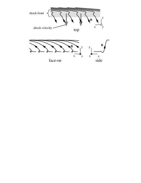
Figure 15: The magnetic field structure in the shock solution plotted in Fig. 14.

The ion and electron velocities approach zero and their densities rapidly increase at $z\approx 0.15\times 10^{15}\,\mathrm{cm}$, at which point large currents prevent further movement to the left in the $B_{x}$–$B_{y}$ phase space (see Fig. 16) and the $B_{x}$ and $v_{x}$ profiles are clipped. The field-line structure of the shock is sketched in Fig. 15.

Figure 16: The phase portraits for the fast shock solutions of Figures 10 (solid), 13 (short-dashed) and 14 (dotted). The long-dashed curve indicates where the ion and electron densities diverge (see text).

The trajectories of the shock solutions are plotted in Figure 16. As expected, the shocks are no longer close to being coplanar, and the upstream state becomes a spiral node, with the magnetic field oscillating ahead of the shock solution. The long-dashed curve shows the locus where the the ion and electron densities diverge, i.e. where $v_{iz}=v_{ez}=0$ (see §3.4). The trajectory for the shock propagating into the $10^{7}\,\mathrm{cm}^{-3}$ gas with 0.1 $\mu$ grains approaches this locus, but is forced away by the associated large current density.

4.3 The effect of the grain-size distribution

In this subsection, I consider the effect of an MRN distribution on the shock dynamics, both with and without an additional population of very small grains. Ionization models of the ambient molecular gas show that at gas densities of order $10^{6}\,\mathrm{cm}^{-3}$, not all grains are charged, but the no. density of those that are is order $10^{-11}{n_{\rm H}}$. Thus, the net charge on the grains, $n_{g}Z_{g}\approx 10^{-11}{n_{\rm H}}$ is of the same order as that for the single-grain-size models presented in the previous subsection, for which $n_{g}/{n_{\rm H}}\approx 10^{-13}$ and $Z_{g}\approx-120$. The shock models are therefore rather similar.

When PAHs are present, they are the dominant charged species. The effects of interest are greatest at densities around $10^{6}\,\mathrm{cm}^{-3}$, as at higher densities the abundances of positively and negatively charged grains become very similar, and $|\sigma_{1}|/\sigma_{2}$ becomes small. For ${n_{\rm H}}=10^{6}\,\mathrm{cm}^{-3}$, the fractional abundances of positively charged PAHs plus ions is $3\times 10^{-9}$, with a similar abundance of negatively charged PAHs. Singly-charged grains and electrons both have abundances of approximately $2\times 10^{-11}$ (Nishi et al. 1991; Kaufman & Neufeld 1996a). Thus I adopt pre-shock densities and magnetic fields ${n_{\rm H}}=10^{6}\,\mathrm{cm}^{-3}$ and $B_{0}=1\,\mathrm{mG}$ and a four fluid model consisting of neutrals, positively and negatively charged ion-like particles each with $n/{n_{\rm H}}=2\times 10^{-11}$, negatively charged grains with $N/{n_{\rm H}}=2\times 10^{-11}$. The two species of ion-like particles are assumed to be identical apart from the sign of their charge, with $<\sigma v>=1.6\times 10^{-9}\,\mathrm{cm}^{-3}\,\mathrm{s}^{-1}$, so their pre-shock Hall parameters are $\pm 4609$. The grains are assumed to satisfy the power-law size distribution (26) between $a_{1}=50$Å and $a_{2}=2500$Å. Given a choice of the pre-shock Hall parameter of the smallest grains, $\beta_{1}$, the effective values of $n_{g}$ and $\beta_{g}$ can be calculated.

Figure 17: Integral curves in the $B_{x}$-$B_{y}$ phase space for shocks with ${n_{\rm H}}=10^{6}\,\mathrm{cm}^{-3}$, $v_{s}/v_{A}=10$, and $\theta=30\degr$, for the case when grain sizes follow an MRN distribution and there is an additional population of PAHs. The different trajectories are labelled by the value of the pre-shock Hall parameter for the smallest grains, with radii of 50 Å (see text).

Rather than show the detailed shock structure, which is similar to that presented previously, I show in Figure 17 the phase-space trajectories for different choices of $\beta_{1}$. As $\beta_{1}$ decreases, $\beta_{g}$ decreases, and $n_{g}$ increases, so the shocks become increasingly non-coplanar, with the characteristic spiral trajectory for $|\beta_{g}|\la 0.3$. This is to be expected from the non-coplanarity criterion (74). These results indicate that significant non-coplanarity occurs for $\beta_{1}\la 1$, that is, in regions of unusually weak field (see eq [3.5]).

In the absence of PAHs, the dominant charged fluids for ${n_{\rm H}}\la 10^{9}\,\mathrm{cm}^{-3}$ are ions, electrons and grains carrying a single negative charge (Nishi et al. 1991). At densities of $10^{6},\,10^{7},\,10^{8}\,\mathrm{cm}^{-3}$, I adopt fractional abundances $n_{i}/{n_{\rm H}}=10^{-9},\,3\times 10^{-10},\,1.03\times 10^{-10}$ and $N/{n_{\rm H}}=3\times 10^{-10},\,2\times 10^{-10},\,1\times 10^{-10}$ respectively. At the two lower densities, the density of electrons is determined by charge neutrality once the charged grain abundance is corrected for the size distribution. At $10^{8}\,\mathrm{cm}^{-3}$, the electron density is relatively small and would be strongly affected by this procedure, so the no. density for charged grains is not corrected for the size distribution. In any case, the corrections would amount to changes of order 5 per cent.

Figure 18: Integral curves in the $B_{x}$-$B_{y}$ phase space for shocks with $v_{s}/v_{A}=10$, and $\theta=30\degr$, for the case when grain sizes follow an MRN distribution and PAHs are absent. The different trajectories correspond to different choices of pre-shock magnetic field and gas density – solid:$1\,\mathrm{mG,\,10^{6}}\,\mathrm{cm}^{-3}$; short-dashed:$0.3\,\mathrm{mG,\,10^{6}}\,\mathrm{cm}^{-3}$ or $3\,\mathrm{mG,\,10^{7}}\,\mathrm{cm}^{-3}$; long-dashed: $1\,\mathrm{mG,\,10^{7}}\,\mathrm{cm}^{-3}$ or $10\,\mathrm{mG,\,10^{8}}\,\mathrm{cm}^{-3}$; dotted: $3\,\mathrm{mG,}\,\,10^{8}\,\mathrm{cm}^{-3}$.

Figure 18 presents the trajectories for shocks with $v_{s}/v_{A}=10$ at these three densities for standard and lower values of the magnetic field. This illustrates how the shock trajectory depends primarily on the ratio $B/{n_{\rm H}}$ that determines the Hall parameters, with the particle abundances and field strength determining the shock thickness.

5 Discussion

The results presented in §4 confirm that both intermediate and fast C-type shock solutions exist. A one-parameter family of intermediate shocks exists for each shock speed between the intermediate speed $v_{A}\cos\theta$ and $\sqrt{2}v_{A}\cot\theta$; at higher speeds the downstream states become unphysical. A unique fast shock exists for each shock speed in excess of the fast speed $v_{A}$. The relationship between these two classes of solution is summarised by the trajectories in the $B_{x}$–$B_{y}$ phase-space diagram.

The fast shock trajectory runs along the $B_{x}$ axis if the charged species are tied to the magnetic field lines, or if positive and negatively charged species have identical abundances and Hall parameters. In this case, integration of the fast shock solution away from the upstream state is straightforward. The direction of the trajectory leaving the upstream stationary point (i.e. along the $B_{x}$ axis) is known, and the velocity and magnetic field vectors in the fast shock solution are confined to the $x$-$z$ plane, so the $y$ components can be discarded. Integration can be started by stepping off U towards F, and then integrating the trajectory (e.g. Draine 1980; Wardle & Draine 1987).

The symmetry of phase space under reflection in the $B_{x}$ axis is destroyed by grains, which being partially decoupled from the magnetic field and preferentially carrying a negative charge, introduce a handedness into the fluid. The fast shock trajectory no longer runs along the $B_{x}$ axis, and this distortion provides an opportunity for numerical mixing of the fast solution with the neighbouring divergent intermediate shock trajectories during integration. Any attempted integration from U to F is doomed. To begin with, there is no a-priori means of determining the direction for the initial step off the point U. In principle this problem could be circumvented by using a shooting method to adjust the starting direction until the integration successfully reached F. However, because of finite numerical precision, any attempted integration into F along the fast trajectory will step onto a neighbouring intermediate shock trajectory and eventually be forced away from the fast trajectory and towards I (c.f. integration towards sonic points). This behaviour prevented Pilipp & Hartquist (1994), who started their integrations at U and treated the direction of the first step away from U as a free parameter, from finding the fast shock solutions. At low shock speeds, they discovered the family of intermediate shocks but could not find the fast shock, noting instead that the sense of rotation of $\mn@boldsymbol{B_{\perp}}$ within the intermediate shocks changed at a critical direction of the initial step away from U. At higher speeds, for which the intermediate shock solutions become unphysical, Pilipp & Hartquist were unable to find any acceptable solutions.

A realistic treatment of the ionization balance is required for a quantitative assessment of the role of grains in C-type shocks. The ionization balance is particularly important when $v_{z}$ for any charged species approaches zero and the number density of that species diverges in the constant-flux approximation (eq. 2) used here. This does not affect the divergence of trajectories from the fast trajectory unless the fast trajectory itself approaches this limit (e.g. the trajectory shown in Fig. 16 for the shock displayed in Fig. 14).

Some conclusions are robust to changes in the microphysics. If the conductivity of the gas can be regarded as some unspecified function of local physical variables at any point within the shock front, so that shock solutions can still be represented as trajectories in the $B_{y}$–$B_{x}$ phase-space, the topology of the phase space is determined by the nature of the fixed points. These were shown in §3.2 to be a source, sink and saddle independent of the conductivity tensor. Thus the integral curves always have the topology plotted in Figure 4, apart from smooth distortions (as apparent in Fig 9) because of changes to the conductivity tensor. The intermediate-shock curves always run from U or D to I, and thus $v_{iz}=v_{ez}=0$ at some point if the shock speed is high enough for intermediate shocks to be excluded. The fast shock trajectory could in principle cross the $v_{iz}=v_{ez}=0$ locus if the ionization balance is able to distort the trajectory sufficiently, although it is apparently unable to do so in the fixed-flux approximation used here (see Fig. 18). In any case, when the fixed-flux condition is dropped, crossing this locus does not imply infinite charged-particle abundances as the increase is limited by recombinations. Intermediate shocks, however, will still be excluded as their downstream conditions are unphysical.

A more realistic treatment of the physical processes occurring within the shock front is essential as the grain properties within the shock and the shock structure itself are intimately related. In particular, the neutral and electron temperatures are required to accurately calculate the Hall parameters for a given grain size. In addition, the grain-size distribution varies within the shock front as different sized grains will generally have different drift speeds, the smallest grains being compressed with the magnetic field, the largest grains with the neutrals. Incorporation of these effects increases the dimensionality of the phase space by introducing differential equations for the temperatures and relative abundances of different species. In principle this could alter the topology of the phase space, although this is unlikely to be the case in practice. There are, however, practical problems in finding the fast shock structure by integrating backwards from the downstream state if chemistry is coupled to the hydrodynamics (through e.g. changing the abundances of coolants or the degree of ionization in the shock), since one does not then know the post-shock conditions a-priori (c.f. the discussion in Roberge & Draine (1990) regarding C^∗- and J-shocks), and a time-consuming shooting method must be employed.

Although the grain drag significantly modifies the shock structure, it is unclear whether this will produce gross differences in the total line emission from the shock front. The essential feature of C-shock structure is that it maintains a layer of hot molecular gas. For a given pre-shock density and shock speed, the same power is dissipated per unit area independently of the detailed structure of the shock front. The gas generally will be heated up to temperatures between 1000 and 2000 K at which point the local heating and cooling balance. Molecules will remain intact and the molecular line emission will not be greatly affected. The insensitivity of line ratios to details of shock structure is illustrated by recent numerical work (Stone 1997; Neufeld & Stone 1997; MacLow & Smith 1997), which follows the development and saturation of the instability in C-type shocks (Wardle 1990). Even though the neutral gas is collected into dense fingers within the shock front, the line ratios are generally unchanged by more than a factor of two (Neufeld & Stone 1997), although diagnostics can be found (MacLow & Smith 1997). Nevertheless, one might expect that the grains will affect the stability of C-shocks and also the speed at which shocks become J-type.

Finally, it is worth pointing out that the theoretical study of C-shocks in molecular clouds will contribute to the general theory of MHD shock waves, and of intermediate shocks in particular (see the review by Wu 1995). Until recently intermediate shocks in MHD were thought to be unphysical because they appeared to lack sufficient freedom to adjust to slight perturbations in the upstream or downstream flow (see, e.g. Kantrowitz & Petschek 1965). The issue was reopened when intermediate shocks emerged as stable structures in numerical simulations (Wu 1988a; Steinolfson & Hundhausen 1990a,b). It has since been realised that the arguments against the existence of intermediate shocks are based on ideal MHD, which breaks down completely within the shock front. Numerical studies of time-dependent intermediate shocks in resistive MHD demonstrated that the shocks could be formed ‘naturally’ and were stable (Wu 1990). An examination of the structure of resistive, intermediate shocks in the weak shock limit (Kennel et al. 1989; Wu & Kennel 1992), shows that, as found for C-type shock waves, for given external parameters (i.e. pre-shock conditions and shock speed), a one-parameter family of intermediate shock structures exist connecting the jump conditions. This ‘internal’ parameter provides the additional freedom for the shock to adjust its structure to external perturbations, a behaviour outside of the scope of ideal MHD in which the shock transition is represented as a discontinuity between the upstream and downstream states. As these conclusions depend on shock structure, in principle they depend on the model used for the magnetised medium. Resistive (Wu 1990) and hybrid (Wu & Hada 1991) models have been investigated so far. With the advent of multidimensional ambipolar diffusion codes, it has become possible to study these issues in weakly ionized media (see Smith & MacLow 1997).

6 Summary

In this paper I constructed steady models of oblique C-type shocks in which the magnetic field within the shock front is not artificially confined to the plane containing the upstream and downstream magnetic field and the shock normal. Four fluids – neutrals, ions, electrons or PAHs, and negatively charged grains – were considered. The thermal pressure of the fluids and the inertia of the charged components were neglected. The effects of chemistry and changes in fractional ionization, and the charge residing on grains were ignored. The rate coefficients for grain-neutral and electron-neutral elastic scattering (which depend in principle on the neutral temperature and the grain-neutral drift speed, and on the electron temperature, respectively) were assumed constant with values appropriate to conditions within the shock front.

These assumptions reduce the number of differential equations describing the shock structure to a pair for the components $B_{x},\,B_{y}$ of the magnetic field that are perpendicular to the shock normal. Shock solutions can therefore be conveniently represented by trajectories in a two-dimensional phase space.

Models were presented for weak shocks ($v_{s}/v_{A}=1.5$), and for strong shocks ($v_{s}/v_{A}=10$). Variations in the grain size from $0.1\mu$ to $0.4\mu$, and the effect of an MRN grain-size distribution were considered.

The results are summarized as follows:

1. The cold MHD jump conditions permit three stationary points in the phase space, corresponding to the upstream state and downstream states of the fast (for $v_{s}>v_{A}$) and intermediate shocks ($v_{A}\,{\rm cos}\,\theta<v_{s}<v_{A}{\rm cot}\,\theta$). Valid shock solutions have phase-space trajectories linking the upstream state to one of the downstream states. A linear analysis, valid for any number of charged species, shows that the upstream state is a source, the fast downstream state is a saddle, and the intermediate downstream state is a sink.

2. A one-parameter family of intermediate shocks exists for each shock speed in the range $v_{A}\,{\rm cos}\,\theta<v_{s}<v_{A}{\rm cot}\,\theta$ where $\theta$ is the angle between the shock normal and the pre-shock magnetic field. These solutions correspond to those found by Pilipp & Hartquist (1994). The family contains members with either sense of rotation of $\mn@boldsymbol{B_{\perp}}$ through the shock front, members with a rarefaction precursor in which $\mn@boldsymbol{B_{\perp}}$ becomes small within the front before compression begins, and members that correspond to a fast shock followed downstream at a finite distance by an intermediate shock.

3. A unique fast shock exists for each shock speed $v_{s}>v_{A}$, where $v_{A}$ is the Alfvén speed in the pre-shock gas. Pilipp & Hartquist (1994) were unable to find these solutions because integration of the equations for shock structure from the upstream state to the downstream state is unstable. Instead, integration must begin at the downstream state and run backwards through the shock front.

4. When all charged particles are well couwell coupled to the magnetic field, or when there is a symmetry between the poorly-coupled particles of either sign, the phase space is symmetric about the $B_{x}$ axis, and the fast shock is coplanar, its trajectory running along the $B_{x}$ axis. In conditions typical of molecular clouds, negatively-charged grains contribute significantly to the drag and are loosely coupled to the field. The net asymmetry in the coupling of negatively and positively charged particles to the magnetic field lines imposes a handedness on the shock structure and the phase space trajectories lose their symmetry on reflection in the $B_{x}$ axis. In particular, the fast shock trajectory no longer runs along the axis – the magnetic field and fluid velocities no longer lie in the $x$-$z$ plane (containing the pre-shock field and shock normal) but have significant $y$ components within the shock front.

5. For typical conditions in molecular clouds, grains dominate the frictional force and the magnetic field is well-tied to ions, electrons and PAHs. Under these conditions for given values of pre-shock magnetic field and gas density, the pre-shock grain Hall parameter determines the shock structure apart from an overall length scale for the shock thickness which is determined by the grain abundance. Thus under the approximations adopted in this paper, the shock structures are relatively insensitive to the details of the grain-size distribution and the exact composition of the charged species in the gas.

6. An MRN grain-size distribution can be approximately incorporated by calculating an effective abundance and an effective grain Hall parameter for single-size grains. The ratio of the effective abundance to the abundance of charged MRN grains, and the effective Hall parameter are determined by the Hall parameter of the smallest grains in the MRN distribution.

7. The degree of noncoplanarity is determined by the grain Hall parameter $\beta_{g}$, with significant effects being found for $|\beta_{g}|\la 1$. When $|\beta_{g}|\la 0.3$ the upstream state becomes a spiral node and the shocks exhibit a precursor in which $\mn@boldsymbol{B_{\perp}}$ may make several rotations.

8. Ions and electrons become passive in the sense that they may stream through the neutral gas with large transverse drift velocities (of order half the shock speed or more) without generating significant dissipation, as the shock thickness is determined by the collisions of neutrals with charged grains. The primary role of these charged species is to guarantee that the electric field in the shock front is very nearly orthogonal to the magnetic field.

9. Supressing the out-of-plane components of the drift velocities and magnetic field may significantly reduce the current and leads to a thicker shock structure (by, e.g. a factor of two) and a consequent decrease in the heating rate within the shock front. Models supressing the out-of-plane components of the magnetic field and velocity therefore underestimate the temperatures within the shock front, and significantly underestimate the magnitude of the grain drift speed through the neutrals.

This work was initiated at the University of Rochester. A. Perez-Miller is thanked for assistance with coding. This research was partially supported by NASA to the University of Rochester through grant NAGW-2444. The Special Research Centre for Theoretical Astrophysics is funded by the Australian Research Council under the Special Research Centre programme.

References

- [] Chernoff, D. F. 1987, ApJ, 312, 143
- [] Chernoff, D. F., Mckee, C. F. & Hollenbach, D. J. 1982, ApJ, 259, L97
- [] Chrysostomou, A., Burton, M. G., Axon, D. J., Brand, P. W. J. L., Hough, J. H., Bland-Hawthorn, J. & Geballe, T. R. 1997, MNRAS, 298, 605
- [] Ciolek, G. E. & Mouschovias, T. Ch. 1993, ApJ, 418, 774
- [] Cowling, T. G. 1957, Magnetohydrodynamics (New York: Interscience)
- [] Cowling, T. G. 1976, Magnetohydrodynamics, 2nd ed (London: Hilger)
- [] Draine, B. T. 1980, Ap J, 241, 1021
- [] Draine, B. T. 1986, MNRAS, 220, 133
- [] Draine, B. T. & Katz, N. 1986a, ApJ, 306, 655
- [] Draine, B. T. & Katz, N. 1986b, ApJ, 310, 392
- [] Draine, B. T. & Lee, H. M. 1984, ApJ, 285, 89
- [] Draine, B. T. & Roberge, W. G. 1982, ApJ, 259, L91
- [] Draine, B. T., Roberge, W. G. & Dalgarno, A. 1983, ApJ, 264, 485
- [] Elmegreen B. G. 1979, ApJ, 232, 729
- [] Flower, D. R., Pineau des Forêts, G. & Hartquist, T. W. 1985, MNRAS, 216, 775
- [] Gear, C. W. 1971, Numerical value problems in ordinary differential equations (Englewood Cliffs: Prentice-Hall)
- [] Gilardini, A. 1972, Low energy electron collisions in gases: swarm and plasma methods applied to their study (New York: Wiley)
- [] Gradshteyn, I. S. & Ryzhik, I. M. 1994, Table of integrals, series, and products, 5th edn (London: Academic Press)
- [] Hartquist, T. W., Pilipp, W. & Havnes, O. 1997, Ap&SS, 246, 243
- [] Kaufman, M. J. & Neufeld, D. A. 1996a, ApJ, 456, 250
- [kn96a] Kaufman, M. J. & Neufeld, D. A. 1996b, ApJ, 456, 611
- [] Kennel, C. F., Blandford, R. D. & Coppi, P. 1989, J. Plasma Physics, 42, 299
- [] Kennel, C. F., Blandford, R. D. & Wu, C. C. 1990, Phys. Fluids B, 2, 253
- [] Königl, A. 1989, ApJ, 342, 208
- [] Léger, A. & Puget, J. L. 1984, AA, 137, L5
- [lm] Li, Z.-Y. & McKee, C. F. 1996, ApJ, 464, 373
- [] MacLow, M.-M. & Smith, M. D. 1997, ApJ, 491, 596
- [] Mathis, J. S., Rumpl, W. & Nordsieck, K. H. 1977, ApJ, 217, 425
- [mch] McKee, C. F., Chernoff, D. F. & Hollenbach, D. J. 1984, in Galactic and Extragalactic Infrared Spectroscopy, ed. M. F. Kessler & J. P. Phillips (Dordrecht : Reidel), 103
- [m87] Mouschovias, T. Ch. 1987, in Physical Processes in Interstellar Clouds, ed. G. E. Morfill & M. Scholer (Dordrecht: Reidel), 491
- [] Mullan, D. J. 1971, MNRAS, 153, 145
- [] Nakano, T., Umebayashi, T. 1986, MNRAS, 218, 663
- [] Neufeld, D. A. & Hollenbach, D. J. 1994, ApJ, 428, 170
- [] Neufeld, D. A. & Stone, J. A. 1997, ApJ, 487, 283
- [] Nishi, R., Nakano, T., Umebayashi, T. 1991, ApJ, 368, 181
- [] Pilipp, W. & Hartquist, T. W. 1994, MNRAS, 267, 801
- [] Pilipp, W., Hartquist, T. W. & Havnes, O. 1990, MNRAS, 243, 685
- [] Pineau des Forêts, G., Flower, D. R. & Hartquist, T. W. 1986, MNRAS, 220, 801
- [] Puget, J. L. & Léger, A. 1989, ARAA, 27, 161
- [] Roberge, W. G. & Draine, B. T. 1990, ApJ, 350, 700
- [] Shu F. H. 1983, ApJ, 273, 202
- [] Smith, M. D. 1992, ApJ, 390, 447
- [] Smith, M. D. & Brand, P. W. J. L. 1990, MNRAS, 245, 109
- [] Smith, M. D. & MacLow, M.-M. 1997, AA, 326, 801
- [] Smith, M. D., Brand, P. W. J. L. & Moorhouse, A. 1991, MNRAS, 248, 451
- [] Steinolfson, R. S. & Hundhausen, A. J. 1990a, JGRA, 95, 6389
- [] Steinolfson, R. S. & Hundhausen, A. J. 1990b, JGRA, 95, 20693
- [] Stone, J. A. 1997, ApJ, 487, 271
- [] Wardle, M., 1990, MNRAS, 246, 98
- [] Wardle M. 1991a, MNRAS, 250, 523
- [] Wardle M. 1991b, MNRAS, 251, 119
- [] Wardle, M. & Draine, B. T. 1987, ApJ, 321, 321
- [] Wu, C. C. 1988a, J. Geophys. Res. A, 93, 987
- [] Wu, C. C. 1988b, J. Geophys. Res. A, 93, 3969
- [] Wu, C. C. 1990, J. Geophys. Res. A, 95, 8149
- [] Wu, C. C. 1995, Physica Scripta, T60, 97
- [] Wu, C. C. & Hada, T. 1991, J. Geophys. Res. A, 96, 3769
- [] Wu, C. C. & Kennel, C. F. 1992, Phys. Rev. Lett. 68, 56