A scalar field matter model for dark halos of galaxies and gravitational redshift

Abstract

We analyze the spherically symmetric Einstein field equation with a massless complex scalar field. We can use the Newtonian solutions to fit the rotation curve data of spiral and dwarf galaxies. From the general relativistic solutions, we can derive high gravitational redshift values.

]

I Introduction

The rotation curves for galaxies or galaxy clusters should show a Keplerian decrease $v\simeq\sqrt{1/x}$ at the point where the luminous matter ends. Instead one observes flat rotation curves beyond the galaxies [1]. A linear radial increase of the mass function of galaxies and galaxy clusters have been derived from these observations [2]: $M=v^{2}_{limit}x$. Several models have been discussed where either non-Newtonian gravity [3] or non-interacting matter, dark matter [4], are introduced to solve this problem. For several classes of gravitational theories, it was recently shown that the introduction of dark matter is necessary [5]; cf. [6]. Massive compact halo objects, so-called MACHOs, consisting of baryonic matter are also not able to solve this problem [7].

In 1933 Zwicky [8] was the first who suggested the existence of dark matter in galaxy clusters by investigating the Coma cluster. The total mass needed to gravitationally bind this cluster exceeds the amount of the luminous matter by roughly an order of magnitude. Three years later Smith proved this for the Virgo cluster [9]. Beginning of the 1970’s one was able to extend the measurements of the rotation curves of galaxies so that higher mass to luminosity relations could be found: after some radius the rotation curves revealed that there is more mass than contained within the luminous matter [10]. The explanation of a linearly increasing mass was first given by Freeman [11] providing a spherical halo. The investigations for determining the radius of a dark matter halo have to go beyond the HI measurements of the 1980’s [12], e.g. by studying satellite galaxies [13], using the weak lensing of background galaxies by foreground dark halos [14], or looking into quasar absorption lines [15]; cf. [16]. From these investigations, halo radii of more than 200kpc are inferred, for our Galaxy 230kpc [17], and recent results from satellite galaxies of a set of spiral galaxies show even more than 400kpc [18]. Recently, measurements of rotation curves of high redshift galaxies have been carried out [19].

We present a solution class of a massless complex scalar field minimally coupled to the Einstein equation [20]. For the Newtonian types of these solutions, we can fit rotation curve data of spiral and dwarf galaxies. The limiting value of the orbital velocity is determined by the central amplitude of the scalar field. The frequency of the scalar field determines the halo characteristics of mass and density near the center.

For the general-relativistic (GR) solutions, we can show that they provide large gravitational redshifts. We discuss how emission and absorption lines produced in the highly relativistic potential of our model can be understood. Near the center of these solutions, we find rotation velocities of about 10⁵km/s so that high luminosities can be expected. Spacetime singularities do not appear within these GR solutions.

A self-gravitationally massive complex scalar field is utilized for the so-called boson stars [21, 22, 23, 24]. These boson stars have no physical singularities as in our solutions or in the case of neutron stars. However, real massless [25] or massive [26] scalar fields (in each case without conserved Noether current) cannot prevent the formation of a singularity (cf. also the exact solution in [27]). Such behavior of singular solutions is supported by analytical investigations of Christodoulou [28] and numerical calculations of Choptuik [29].

II Einstein-scalar-field equations

The Lagrange density of a massless complex self-gravitating scalar field reads

$${\cal L}=\frac{1}{2}\sqrt{\mid g\mid}\left[\frac{1}{\kappa}R+g^{\mu\nu}(\partial_{\mu}\Phi^{\ast})(\partial_{\nu}\Phi)\right]\;,$$ (1)

where $R$ is the curvature scalar, $\kappa=8\pi G$, $G$ the gravitation constant ($\hbar=c=1$), $g$ the determinant of the metric $g_{\mu\nu}$, and $\Phi$ the massless complex scalar field. Then we find the coupled system

$$R_{\mu\nu}-\frac{1}{2}g_{\mu\nu}R = -\kappa T_{\mu\nu}(\Phi)\;,$$ (2)

$$\Box\Phi = 0\;,$$ (3)

where

$$T_{\mu\nu}=(\partial_{\mu}\Phi^{\ast})(\partial_{\nu}\Phi)-\frac{1}{2}g_{\mu\nu}[g^{\sigma\kappa}(\partial_{\sigma}\Phi^{\ast})(\partial_{\kappa}\Phi)]$$ (4)

is the energy-momentum tensor and

$$\Box=\partial_{\mu}\Bigl{[}\sqrt{\mid g\mid}g^{\mu\nu}\partial_{\nu}\Bigr{]}/\sqrt{\mid g\mid}$$ (5)

the generally covariant d’Alembertian.

For spherically symmetric solutions we use the following static line element

$$ds^{2}=e^{\nu(r)}dt^{2}-e^{\lambda(r)}dr^{2}-r^{2}(d\vartheta^{2}+\sin^{2}\vartheta\,d\varphi^{2})$$ (6)

and, for the scalar field, the ansatz

$$\Phi(r,t)=P(r)e^{-i\omega t}\;,\\$$ (7)

where $\omega$ is the frequency of the scalar field.

The non-vanishing components of the energy-momentum tensor are

$$T_{0}{}^{0} = \rho=-T_{1}{}^{1}=p_{r}$$ (8)

$$= \frac{1}{2}[\omega^{2}P^{2}(r)e^{-\nu}+P^{\prime 2}(r)e^{-\lambda}]\;,$$ (9)

$$T_{2}{}^{2} = T_{3}{}^{3}=-p_{\bot}$$ (10)

$$= -\frac{1}{2}[\omega^{2}P^{2}(r)e^{-\nu}-P^{\prime 2}(r)e^{-\lambda}]\;,$$ (11)

where ${}^{\prime}=d/dr$. As equation of state, we find $\rho=p_{r}=p_{\bot}+P^{\prime 2}(r)e^{-\lambda}$.

The decisive non-vanishing components of the Einstein equation are

$$\nu^{\prime}+\lambda^{\prime} = \kappa(\rho+p_{r})re^{\lambda}\;,$$ (12)

$$\lambda^{\prime} = \kappa\rho re^{\lambda}-\frac{1}{r}(e^{\lambda}-1)\;,$$ (13)

and two further identical components which are fulfilled because of the Bianchi identities.

The differential equation for the scalar field is

$$P^{\prime\prime}(r)+\left(\frac{\nu^{\prime}-\lambda^{\prime}}{2}+\frac{2}{r}\right)P^{\prime}(r)+e^{\lambda-\nu}\omega^{2}P(r)=0\;.$$ (14)

A typical behavior of the scalar field of Newtonian kind is demonstrated in Fig. 1; the metric potentials are almost constant so that we do not show them here; cf. Section III. General relativistic solutions are shown in Section IX.

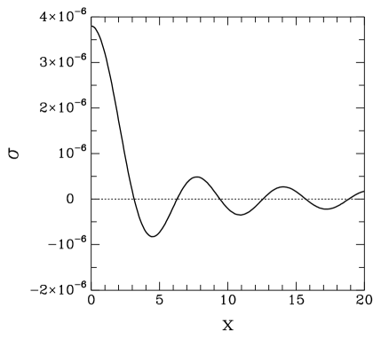
FIG. 1.: The massless complex scalar field $\sigma=\sqrt{\kappa/2}\,P$ depending on the dimensionless coordinate $x=\omega r$ with the initial values $\sigma(0)=3.8\times 10^{-6}$ $[\sigma(0)(x_{opt})]$ and $\nu(0)=0$. This solution belongs to the rotation curve with $M_{I}=-18.29$ in Fig. 4.

For the rest of our paper, we employ the redefined quantities $x:=\omega r$ and $\sigma:=\sqrt{\kappa/2}\;P$. The numerical calculation was carried out by using a Runge-Kutta-routine of the Fortran-libraries IMSL/NAg. In order to get regular solutions at the origin for the system of differential equations (12), (13), and (14), we have to put the initial conditions $\sigma^{\prime}(0)=0$ and $\lambda(0)=0$.

The system (12), (13), and (14) possesses the self-similarity: $x\rightarrow kx$, $\lambda\rightarrow\lambda$, $e^{\nu}\rightarrow k^{2}e^{\nu}$, and $\sigma\rightarrow\sigma$. This self-similarity means that one has only one free parameter, namely the initial value of the scalar field. One scales the solution simply with the second initial value for $\nu$.

III Newtonian solution

The Newtonian solutions of our Lagrangian (1) are characterised by almost constant metric potentials $\nu,\lambda$. The scalar field equation (14) can then be rewritten into the following form:

$$\sigma^{\prime\prime}+\frac{2\sigma^{\prime}}{x}+\sigma=0\;,\\$$ (15)

(${}^{\prime}=d/dx$) which has the solution

$$\sigma(x)=\frac{1}{x}\left[A\sin(x)+B\cos(x)\right]\;,$$ (16)

where $A,B$ are some constants. For $B\neq 0$, the solution is singular at the origin, why we can rule out it.

The Newtonian form of the energy density reads

$$\rho(x)=\frac{A^{2}}{x^{2}}\left[1-\frac{\sin(2x)}{x}+\frac{\sin^{2}(x)}{x^{2}}\right]\;.$$ (17)

For small $x$, we have $\rho\propto A^{2}[1-2x^{2}/9+x^{4}/45]$, i.e. it is proportional to a constant. For dwarf galaxies, one observes such a behavior of the density [30] where good fitting results are obtained by using the empirical isothermal density profile $\rho(x)\propto 1/(x_{c}^{2}+x^{2})$, where $x_{c}$ is the core radius. Hence, our constant $A$ resembles a core radius. By applying a maximum halo model, i.e. without baryonic matter, the value of $A$ is higher than for a model including baryonic matter. Therefore the core radius increases if one adds baryonic matter as found in [30]; cf. [31].

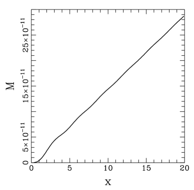
FIG. 2.: The mass function in units of $[\sigma^{2}(0)(x_{opt})/(\omega\kappa)]$ increases near the center like $x^{3}$ and at higher radial values linearly. We use here the same initial values as in Fig. 1, so that this curve shows the behavior of mass for the rotation curve with $M_{I}=-18.29$ in Fig. 4.

The general solution of Eq. (13) is

$$e^{-\lambda}=1-\frac{M(x)}{x}$$ (18)

with the mass function $M(x)=\int_{0}^{x}\rho(\zeta)\zeta^{2}d\zeta$. We find the Newtonian formula (cf. Fig. 2)

$$M(x)=A^{2}\left\{x+\frac{\cos(2x)-1}{2x}\right\}\;.$$ (19)

Comparing with the expected Newtonian result $M=v^{2}_{limit}x$, we see that $v_{limit}=A$; hence, the amplitude of the scalar field at the origin determines the limiting orbital velocity. For small $x$, the mass function behaves like

$$M(x)\propto A^{2}x^{3}/3-2A^{2}x^{5}/45+{\cal O}(x^{7})\;.$$ (20)

This corresponds to the constant density at the center. At higher radial distances, the mass function shows the linear behavior.

Asymptotically, following (18), the metric potential $e^{-\lambda}$ approaches the value $C^{2}:=1-A^{2}$, where $C^{2}<1$. After a redefinition of the coordinate $x\rightarrow C^{-1}x\;,$ the asymptotic space has a deficit solid angle. The area of a sphere of radius $x$ is not $4\pi x^{2}$, but $4\pi C^{2}x^{2}$; cf., e.g., analogous results for global monopoles and global textures [32] where one also finds a linear increase of the mass function. We show in Sections VII and VIII how one can find a closure of the solutions and avoids this asymptotic problem.

Following (12), the second metric potential behaves asymptotically like $e^{\nu}\rightarrow x^{K}$, where $K=2A^{2}/C^{2}=2(1/C^{2}-1)>0$. The behavior of both metric potentials could be confirmed numerically.

A question is the validity of the formulas (16), (17), and (19). We found for $\sigma(0)=10^{-3}$ and $\nu(0)=0$ at $x=10$ a deviation of 0.001%, at $x=100$ of 0.3% and at $x=1000$ of about 4% . This shows clearly that these formulas should be used only near the center. All figures in this paper were produced by using the numerical solutions. If one is interested into the asymptotic behavior of the solutions, the formulas can still be used asymptotically (e.g. for the calculation in the Tables) because one can still derive the order of magnitude from them as we confirmed numerically. For higher intial values of $\sigma$, only numerically determined solutions can be used.

IV Rotation curves

In this Section we shall model rotation curves of dwarf and spiral galaxies. Observations show that rotation curves are becoming flat (constant orbital velocity) in the surrounding region of galaxies where data are received from the 21cm wavelength of neutral hydrogen (HI). But the mass density of the neutral hydrogen is not sufficient to explain this velocity behavior. Therefore, we introduce dark matter consisting of a massless complex scalar field which interacts with the luminous matter exclusively by the gravitational force. We apply only Newtonian solutions of our model.

For the static spherically symmetric metric (6) considered here, circular orbit geodesics obey

$$v_{\varphi}^{2}=\frac{1}{2}r\nu^{\prime}e^{\nu} = \frac{1}{2}e^{\nu}(e^{\lambda}-1)+\frac{1}{2}\kappa p_{r}r^{2}e^{\lambda+\nu}$$ (21)

$$\simeq \frac{M(r)}{r}+\frac{1}{2}\kappa p_{r}r^{2}e^{\lambda+\nu}$$ (22)

which reduces outside of matter for a weakly gravitational field into the Newtonian form $v_{\varphi,Newt}^{2}=M(r)/r$. But, for $p_{r}\neq 0$, we have to use the general-relativistic formula. By using the Newtonian solutions of Section III within (22), we find

$$v_{\varphi}^{2}=A^{2}\left[1-\frac{\sin(2x)}{2x}\right]\;;$$ (23)

cf. a generic rotation curve in Fig. 3.

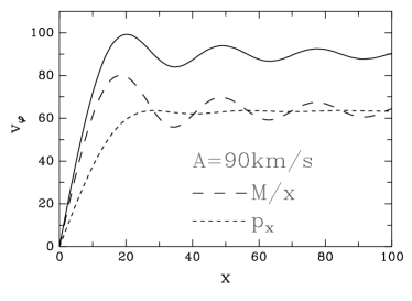
FIG. 3.: A generic rotation curve for an initial value of the scalar field $\sigma(0)=A=3\times 10^{-3}$. The Newtonian (M/x) and the pressure (p_x) contributions are shown separately. In the rotation curve fits, mainly the first part up to the maximum is used. The rotation curve oscillates around the asymptotic value of 90km/s. The velocity $v$ is measured in [km/s] while the dimension of the radial coordinate $r$ depends on the choice of $\omega$; $x$ is dimensionless.

Asymptotically, from (22), we have

$$v_{\varphi}^{2}=e^{\nu}[A^{2}/2+A^{2}/2]$$ (24)

what means that both the first Newtonian part $e^{\nu}(e^{\lambda}-1)/2$ and the second matter part contribute the same amount to the rotation velocity. For $e^{\nu}=1$, we have $v_{\varphi}=A$ as we had already derived from the general Newtonian solution for the mass function.

The next step is now to take observational data for spiral and dwarf galaxies and try to model them by using our model and a model which describes the luminous matter distribution. For spiral galaxies, we use both the universal rotation curves of Persic, Salucci, and Stel [33] and some individual ones. Persic et al. confirmed by investigating data of 967 spirals that the structural properties of dark and visible matter are linked together. This means that a spiral galaxy with low luminosity is stronger dominated by a dark matter halo than a spiral one with high luminosity. This is also one possible statement of the Tully-Fisher relation [1]. From this, it follows that a low luminosity spiral has a rather increasing rotation curve and a high luminosity spiral galaxy a rather decreasing rotation curve.

FIG. 4.: Eight universal rotation curves with different absolute magnitudes $M_{I}$ introduced in [33]. The radial coordinate $x$ in units of the optical radius $x_{opt}$ which encompasses 83% of the total integrated light and the velocity $v$ in units of $v(x_{opt})$. For the halo (long-dashed curve), the initial values are: $\sigma(0)={3.8,3.5,3.3,3.1,2.7,2.4,1.9,1.6}\times 10^{-6}$ of $M_{I}=-18.29$ for the first and $M_{I}=-23.08$ for the last value.

In the following, we model the universal rotation curves by a combination of a stellar disk and our halo. The rotation curve for the stellar disk follows from an exponential thin disk light distribution [33]

$$v_{disk}^{2}(x)/v^{2}(x_{opt})$$ (25)

$$\;=\left[0.72+\frac{0.325}{2.5}(M_{B}^{\ast}-M_{B})\right]\frac{1.97x^{1.22}}{(x^{2}+0.78^{2})^{1.43}}\;,$$ (26)

where $M_{B}^{\ast}=-20.5$ is the absolute magnitude in the blue band (corresponding to $\log L_{\ast}=10.4$) and $M_{B}=-0.38+0.92M_{I}$ ($M_{I}$ from the $I$ band); this formula can be used within the range $0.04\simeq x/x_{opt}\leq 2$. The $x$ depending factor arrives from approximations of modified Bessel functions (see below); the constants in the $M_{B}$ depending factor are arranged that it gives the best fit for our universal rotation curves; cf. [33]. The total rotation curves result then from

$$v_{total}=\sqrt{v_{disk}^{2}+v_{halo}^{2}}\;.$$ (27)

The outcome can be seen in Fig. 4. One recognizes a very good agreement of the data.

From this fit, we find that the amount of disk matter has to decrease with decreasing luminosity, i.e. decreasing absolute magnitude. This is a consequence of the Tully-Fisher relation, but is verified here by fitting the data. From [33], it follows that the rotation curves are self-similar, i.e. only one parameter, the luminosity or the limiting rotation velocity, establishes completely the properties of the halo far from the luminous matter region. This property is also revealed in our model where asymptotically only the parameter $A$ determines the halo; cf. the Newtonian solutions of Section III. Moreover, we can connect this one free parameter with the amplitude of the scalar field at the center.

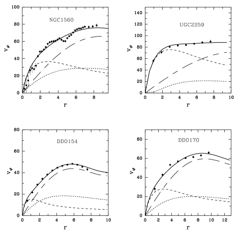
FIG. 5.: Dwarf galaxies: Rotation curve fits for NGC1560, UGC2259, DDO154, and DDO170 with halo (long-dashed), stars (dashed), and HI gas (short-dashed). The velocity $v$ is measured in [km/s] and the radial coordinate $r$ in [kpc]. The parameters for these fits are summarized in Table I.

With the improvements of measuring rotation curves, HI rotation curve data have been found, investigating higher distances from the galaxy center. For an exponentially thin matter disk with a surface density $\Sigma(x/x_{0})=\Sigma_{0}\exp(-x/x_{0})$, where $x_{0}$ is the disk scale length and $\Sigma_{0}$ some constant at $x_{0}$, the contribution to the rotation velocity can be determined by [11] (cf. also [34])

$$v_{disk,gas}^{2}(r)=\frac{\kappa\Sigma_{0}r^{2}}{8r_{0}}\times$$ (28)

$$\left[I_{0}\left(\frac{r}{2r_{0}}\right)K_{0}\left(\frac{r}{2r_{0}}\right)-I_{1}\left(\frac{r}{2r_{0}}\right)K_{1}\left(\frac{r}{2r_{0}}\right)\right]\,,$$ (29)

where $I_{n}$ and $K_{n}$ are modified Bessel functions. Equation (26) is actually the approximation of this exact result. This formula shall be used in the following for the contribution of stars and gas in individual galaxies, with specific constants $r_{0}$ and $\Sigma_{0}$. The gas part contributes with a summand $v_{gas}^{2}$ under the square root in (27).

In some galaxies, a clear bulge can be read off the light curve. For these cases, we use the formula from Kent [35] in order to calculate the circular velocities from the observed surface density $\sigma_{bulge}(r)$

$$v_{bulge}^{2}(r)=\frac{\kappa}{4r}\int\limits_{0}^{r}\zeta\sigma_{bulge}(\zeta)d\zeta+$$ (30)

$$\frac{\kappa}{2\pi r}\int\limits_{r}^{\infty}\left[\arcsin\left(\frac{r}{\zeta}\right)-\frac{r}{\sqrt{\zeta^{2}-r^{2}}}\right]\zeta\sigma_{bulge}(\zeta)d\zeta\,.$$ (31)

Corrections for flattening of bulges are ignored by this formula.

The galaxies we choose belong to a sample of 11 galaxies of different Hubble types and absolute magnitudes which fulfill several strong requirements [36]. All rotation curve data are measured in the 21-cm line of neutral hydrogen, so that the gas distribution extends far beyond the optical disc (at least 8 scale lengths) and the necessity of dark matter is becoming obvious. Isolation of galaxies are another constraint so that perturbative effects of nearby situated galaxies are negligible. Besides of that, high quality data are required.

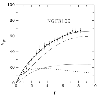
FIG. 6.: Dwarf galaxy: Rotation curve fit for NGC3109 with halo (long-dashed), stars (dashed), and HI gas (short-dashed). The velocity $v$ is measured in [km/s] and the radial coordinate $r$ in [kpc]. The parameters for this fit are summarized in Table I.

For the calculation of the neutral hydrogen gas for the galaxies of this sample, a further remark is in order. In [37], it was shown that the HI data can be decomposed into a sum of two or three exponential disks. We shall use the results of this paper. We start now fitting dwarf galaxies.

TABLE I.: Data for rotation curve fits: luminosity L, disk scale length $r_{0}$, scalar field frequency $\omega$, mass-to-light ratio for disk and bulge, initial value of the scalar field $\sigma$. In all cases, we have used $\nu(0)=-5\times 10^{-6}$. The parameters for the decomposed HI gas surface densities can be found in [37]; we have multiplied the total NGC3109 HI mass by a factor of 1.67 because of some missing 21 cm line flux at the VLA where the NGC3109 observations were made [42, 36]. [Hubble parameter $H_{0}=75$ km/(s Mpc)].

	L	$r_{0}$	$\omega^{-1}$	(M/L)d	(M/L)b	$\sigma(0)$
	[109M⊙]	[kpc]	[kpc]			[$10^{-4}$]
$DDO154$	0.05	0.50	2.6	1.4	—	1.325
$DDO170$	0.16	1.28	4.0	3.7	—	1.8
$NGC1560$	0.35	1.30	4.0	3.0	—	2.0
$UGC2259$	1.02	1.33	5.0	4.5	—	2.2
$NGC2403$	7.90	2.05	9.0	2.0	—	3.5
$NGC2903$	15.3	2.02	9.0	3.5	—	4.4
$NGC2998$	90.0	5.40	1.8	0.25	1.5	5.9
$NGC3109$	0.81	1.55	4.0	0.4	—	1.8
$NGC3198$	9.00	2.63	14.0	3.83	—	3.87
$NGC7331$	54.0	4.48	20.0	2.25	1.7	6.0

Dwarf galaxies have the characteristic of very low luminosities [30]. Following empirical models, their rotation curves vary from the ones of spiral galaxies in such a way that instead of the Hernquist profile [38] an isothermal density profile has to be applied [30]; cf. also [39]. From the rotation curves, it can be derived that the dark matter density near the center is almost constant, i.e. dark matter has a core in these galaxies. Our Newtonian solutions for the massless complex scalar field reveal a constant density near the center, so it is not surprisingly that good fits for five dwarf galaxies from the Begeman et al. sample have been found (Fig. 5 and 6) [40, 41, 42, 43]. In all cases, it is recognizable that the dark matter halo dominates the luminous parts of the galaxies. Especially remarkable is the maximum of the DDO154 data which can be matched perfectly by our dark matter halo; hence, decreasing rotation curve data, at the end of observational resolution, can be explained by using only a dominating dark matter component. The prediction of our model is to find oscillations in rotation curve data at high distances from the center of galaxies.

Our results for the sample of spiral galaxies are summarized in Fig. 7, cf. [43, 44]. In all cases, we are able to produce good fits. Models using an approximate isothermal sphere or a modified Newtonian dynamics (MOND) were also applied for these galaxies, e.g. [45, 36]. Conformal gravitation theory has been explored in [27, 47, 37, 48]; the disadvantage of that model is its increasing rotation curves.

FIG. 7.: Spiral galaxies: Rotation curve fits for NGC2403, NGC2903, NGC3198, and NGC7331 with halo (long-dashed), stars (dashed), and HI gas (short-dashed); NGC7331 has also a bulge included which is truncated at 6.2kpc [43]. The velocity $v$ is measured in [km/s] and the radial coordinate $r$ in [kpc]. The parameters for this fit are summarized in Table I.

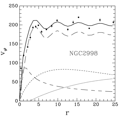
FIG. 8.: Spiral galaxy with oscillating rotation curves: NGC2998 with dominating halo (long-dashed), stars (short-dashed), HI gas (dotted), and bulge (dashed). The velocity $v$ is given in [km/s] and the radial coordinate $r$ in units of [kpc]. In order to find a good correspondence with the data it was necessary to have a dominating halo. The extrema of data and halo are at about the same values of $r$. The bulge is truncated at 2.9kpc; the data for the bulge are taken from [35], but notice a different value for the Hubble constant there. The HI gas contribution [46] was decomposed into $\sigma_{HI}=55\exp(-r/12\mbox{kpc})-49\exp(-r/9\mbox{kpc})$ [M_⊙/pc²]. For other parameters, see Table I.

By building universal rotation curves, a smoothing method is used [33]. Important informations about the distribution of the dark matter within individual rotation curves could be lost by this method. One can find an oscillating behavior within the optical rotation curves of some galaxies, for example NGC2998 [49]; cf. ‘ripples’ in the light curve profile [35]. The explanation is that across a spiral arm, positive velocity gradients are observed; the velocity decrease from the outer edge of one arm to the inner edge of the next arm is in some galaxies faster than Keplerian what is taken as compelling evidence for noncircular velocities. In Fig. 8, we fit the rotation curve data from Rubin et al. [49]. We have taken into account four components: A truncated bulge, a thin disk of stars, an HI component, and a dominating dark halo. What one can recognize is that the data are not fit too well but that the maxima and minima of the fit and the data are at the same place. The dark halo has to be the main part in order to find a good fit. (The partly non-smooth behavior of the curves results from numerical problems because of the scaling of our solution by the scalar field frequency $\omega$.) Further investigations will show whether cylindrically or axisymmetric solutions can improve the fit or rule out our model. NGC2998 belongs to a sample of further 22 spiral galaxies for which the MOND model was applied [50]. Oscillations (‘wiggles’) have been found also in H$\alpha$ rotation curves [51].

V Scaling of the solutions and the mass distribution

As we have seen from the redefined quantity $x=\omega r$, the frequency $\omega$ scales the physical dimension of the solution. Additionally, the mass is scaled with $1/\omega$ and the energy density with $\omega^{2}$. Table II shows for different values of $\omega$ the mass and the density at different radii.

There exist two ways how one can interpret the values of Table II. The last row ($\omega=10^{-21}$/cm) shows a halo having a central density of 10^-21g/cm³; at $x=20$ which means $r=20$kLy the density decreases to a value of 10^-23g/cm³ and within a sphere of this radius the halo has a mass of 10⁴³g$=10^{10}M_{\odot}$.

TABLE II.: Order-of-magnitude estimation for $A=10^{-3}$. We put the frequency $1/\omega=$ 1cm, 10¹⁵cm (about the radius of our solar system), 10¹⁸cm = 1Ly, and 10²¹cm = 1kLy. Further: $\omega$ in units of eV; density $\rho$ at the center and at a distance of $x=20$; the mass within a sphere of radius $x=20$.

$\omega[1/cm]$	$\omega[eV]$	$\rho(0)[g/cm^{3}]$	$\rho(20)[g/cm^{3}]$	$M(20)[g]$
$1$	$10^{-5}$	$10^{21}$	$10^{19}$	$10^{24}$
$10^{-15}$	$10^{-20}$	$10^{-9}$	$10^{-11}$	$10^{37}$
$10^{-18}$	$10^{-23}$	$10^{-15}$	$10^{-17}$	$10^{40}$
$10^{-21}$	$10^{-26}$	$10^{-21}$	$10^{-23}$	$10^{43}$

But one can use Table II also in the vertical direction. A solution with $\omega=1$/cm (first row) has within a sphere of radius 20cm a mass of 10²⁴g, within a sphere of $20\times 10^{15}$cm (20 times the diameter of our solar system; second row) a mass of 10³⁷g, within a sphere of 20Ly (third row) a mass of 10⁴⁰g, and so on. The same procedure is valid for the density columns. The reason why one can do this is that one has a $\omega$ independence of the density and the mass at high radii, but a $\omega$ dependence for small radii. For the mass (19), we find

$$M(r)=\frac{4\pi}{\kappa}A^{2}\left\{r+\frac{\cos(2\omega r)-1}{2\omega^{2}r}\right\}\;,$$ (32)

which goes over for small $r$ values into

$$M(r)\propto\frac{4\pi}{\kappa}A^{2}\left\{\frac{1}{3}\omega^{2}r^{3}-\frac{2}{45}\omega^{4}r^{5}\right\}\;.$$ (33)

The same is valid for the density $\rho$. This result shows that the parameter $A$ determines the behavior of the halo at high distances from the center (namely the limiting orbital velocity), but near the center also the frequency of the scalar field influences the behavior of the mass and the density. Rewriting Eq. (32) into

$$2\omega^{2}r\left[\frac{\kappa M(r)}{4\pi}-A^{2}r\right]=\cos(2\omega r)-1$$ (34)

we immediately see that the left hand side has to be non-positive from which we can find the inequality

$$\frac{\kappa}{4\pi}\frac{M(R)}{R}\leq A^{2}\;,$$ (35)

at an arbitrary radius $R$. This inequality states that at every radius $R$, the relation between the Schwarzschild radius and the radius of the object is smaller than the square of the central value of the scalar field which is 10^-6 for a galaxy with $v_{max}=300$km/s.

Let us, for example, take the value $\omega=10^{-21}$/cm of the last row of Table II. To calculate the mass and the density for smaller radii, we have to take the formulae (17) and (19). The result can be seen in Table III. We recognize in comparison with the values of Table II substantial smaller values.

TABLE III.: Order-of-magnitude estimation for $\omega=10^{-21}$/cm. In comparison with Table II, we find smaller densities and masses at smaller distances.

distance to center	$\rho[g/cm^{3}]$	$M[g]$
20 cm	$10^{-21}$	$10^{-17}$
20 10-3 Ly	$10^{-21}$	$10^{28}$
20 Ly	$10^{-21}$	$10^{37}$
20 kLy	$10^{-23}$	$10^{43}$

The order of magnitude values of Table III for the mass and the density show also a possibility of a hierarchy of objects. Recently [52], it has been detected that the dark matter distribution in the Fornax cluster of galaxies is a mixture of two distinct components on different scales (not necessary distinct matter components). One part is associated with the cluster and the second smaller one with the galaxy NGC1399. This observation was done by looking into the X-ray-emitting diffuse plasma of temperatures 10⁷-10⁸K which is widely found in elliptical galaxies and clusters of galaxies. This gas is likely to be in hydrostatic equilibrium, where the thermal pressure is balanced by the gravity of the cluster. In this way, the X-ray emission traces the distributions of the dark matter in regions of higher density where more gas is trapped. This observation is the first evidence for a hierarchical nature of the dark matter distribution. Future investigations will show whether two of our dark matter halos can be combined: one for the cluster, the other for the single galaxies.

VI Energy density, tangential pressure, and regularity

An investigation of the energy density $\rho$ (i.e. the radial pressure $p_{r}$) shows a terraced decrease (Fig. 9). Furthermore, we find the relation $\mid\rho\mid$ $\geq$ $\mid p_{\bot}\mid$, where the tangential pressure $p_{\bot}$ oscillates sinusoidally around zero. From the equation of state, one recognizes that at each extremum of the scalar field $\sigma$ the difference between radial and tangential pressure vanishes. Hence, at constant spheres, the equation of state $\rho=p$ of a stiff fluid arises.

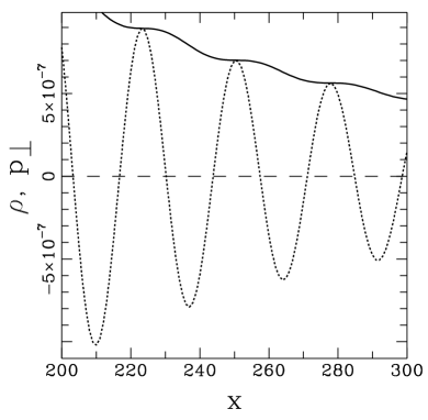
FIG. 9.: The energy density $\rho$ (solid curve) and the tangential pressure $p_{\bot}$ (dotted curve) [both in units of $\omega^{2}/\kappa$] for the interval of $x=200$ up to $x=300$. One recognizes very clearly the terraced decrease of the energy density. The matter behaves like stiff matter at the saddle points of $\rho$. [Initial values: $\sigma(0)=1$ and $\nu(0)=1$]

We check numerically the quadratic curvature invariant (Kretschmann scalar) $R_{inv}^{2}=R^{\lambda\sigma\mu\nu}R_{\lambda\sigma\mu\nu}$ revealing its global regularity for our solutions [20]. The same was found for the two invariants $R_{\mu\nu}R^{\mu\nu}$ of the Ricci tensor and $R^{2}$ of the curvature scalar. The invariants of the irreducible decomposition of Riemann’s curvature tensor show also no singularity [20]. Hence our solutions possess no physically relevant singularity.

VII Construction of a surface

A massive complex scalar field with mass $m$ can be used for constructing a surface of our halo. This massive scalar field has an exponentially decrease and produces a finite mass. We have two different coordinates $x_{1}=mr_{1}$ for the surface with the massive complex scalar field and $x_{2}=\omega r_{2}$ in the interior with the massless complex scalar field. At the connection we require $x_{1}=x_{2}$, hence $\omega/m=r_{1}/r_{2}$. We need an equilibrium of the radial pressures and continuity of the metric potentials. Because of the different scalings in the two regions, we find for the radial pressures $\omega(2)/m=\sqrt{p_{r}(1)/p_{r}(2)}$ [argument $(1)$, e.g. in $\omega(1)$, describes the model of massive complex scalar field and argument $(2)$ that of the massless one], i.e., if we have the equality of the metric potentials, the relation between the pressures gives us the relation between the frequency of the massless scalar field and the mass of the massive scalar field. It was possible to find numerically such solutions, for example: Initial values for the interior region: $\sigma(0)=0.2333,\nu(0)=-0.4055$; for the surface region: $\sigma(0)=0.1,\nu(0)=-0.14035418$; equality for the metric potentials was looked for at $x=3$ and we find $\omega(2)/m=0.3203$. Within the surface, the metric potentials of the massive scalar field go over to the Schwarzschild metric. Hence, we have an object with a finite mass. In the next Section, we shall show another possibility to stop the halo.

TABLE IV.: This table shows the radius $R$ at which our dark matter halo reaches the density $\rho$. $v$ is the limiting orbital velocity.

$\sigma(0)$	$v[km/s]$	$\rho[g/cm^{3}]$	$R[Mpc]$
$10^{-3}$	$300$	$10^{-29}g/cm^{3}$	$2.3$
		$10^{-34}g/cm^{3}$	$830$
$4\times 10^{-4}$	$120$	$10^{-29}g/cm^{3}$	$0.9$
		$10^{-34}g/cm^{3}$	$330$

VIII Cover for the halo

The energy density $\rho$ of the Newtonian solution decreases in leading order as $A^{2}/x^{2}$. Therefore, we can come to the conclusion that the energy density will eventually attain an hydrostatic equilibrium with another matter form at the same pressure value, e.g. the cosmic microwave background radiation (CMBR), which is about 10^-34g/cm³ (seas of neutrinos and supersymmetric particles would increase this density). Alternatively, a cosmological constant $\Lambda$ of the order of magnitude 10^-29g/cm³ would produce much smaller halos; for estimates of $\Lambda$ see [53]. From Table IV, we derive a radius of about 10⁶pc for $\Lambda$ and about 10⁸pc for the CMBR value (cf. the discussion in [54]). Recent observations show halo radii of about 400kpc [18]. Outside the halo, within the spacetime with a constant density, we have a Schwarzschild-de-Sitter metric.

IX Gravitational Redshift and rotation velocity

By increasing the initial value of the scalar field $\sigma(0)$, the Newtonian description breaks down, i.e. the formulae from Section III are no longer valid. The metric potentials $\nu$ and $\lambda$ are not constant and the full nonlinearity of Einstein’s theory has to be taken into account.

The mass and the density function change their behavior smoothly. They still increase together with $\sigma(0)^{2}$ but one recognizes an additional decrease of the $x$ dependent terms; Table V shows the deviation from Newtonian behavior for the mass function with increasing $\sigma(0)$. This means that one can still use the order of magnitudes of Table II (which was for $\sigma(0)=10^{-3}$) but one has to multiply the values of the mass and the density by 10⁴ for $\sigma(0)=0.1$ and by 10⁶ for $\sigma(0)=1$, for example. The deviation of the formula is so eminent that one has to use numerical calculations.

TABLE V.: Deviation for $M/\sigma^{2}(0)$ from the Newtonian formula (19) with increasing $\sigma(0)$; the mass still increases with $\sigma(0)$. The values for $x=0.1$ have to be multiplied by $10^{-3}$.

$x$	Newtonian	$\sigma(0)=0.1$	0.5	1.0	1.5
$0.1$	0.33288	0.33287	0.33255	0.33156	0.32991
$1.0$	0.291	0.290	0.267	0.212	0.154
$2.0$	1.586	1.571	1.261	0.747	0.422
$3.0$	2.993	2.955	2.235	1.193	0.633
$4.0$	3.856	3.798	2.799	1.513	0.811
$5.0$	4.816	4.715	3.166	1.739	0.972

The strong curvature connected with these general relativistic (GR) solutions produces also a gravitational redshift $z$ which, for a static spherically symmetric mass distribution, is given by

$$z=e^{[\nu(A_{1})-\nu(A_{0})]/2}-1\;,$$ (36)

where $A_{0}$ corresponds to the place of the emitter and $A_{1}$ to that of the receiver, both in rest. Table VI shows results for different values of $\sigma(0)$ up to $x=500$. The redshift increases with growing $\sigma(0)$ and with growing radius. Redshift values reached by a(n emitting) gas cloud at the center of the halo can achieve very high values; we have not found numerically any limits. The $z$ values for different $x$ show the gravitational redshift which appears if our GR halo ends at $x$. In Table VII, we assume that the gas clouds are in rest within the gravitational halo potential (more likely they circulate around the center so that an additional Doppler redshift has to be taken into account). Then, the redshifts can be interpreted as emission or absorption lines of the corresponding gas clouds. An interpretation of both Tables could be (for $\sigma(0)=1.0$): Some radiation comes from the center and is gravitationally redshifted by $z=4.76$, some part of the radiation is absorbed from a gas cloud at a distance $x=1$ ($z=3.398$), another part at $x=100$ ($z=0.087$), and finally the halo ends at $x=500$ so that gravitational redshift does not take any further effect. Near the center ($x=1$), we recognize a steep decrease of redshift values (cf. Table VI and VII). The scale of such a halo is again defined by the frequency $\omega$. If one assumes $\omega=10^{-18}$/cm, then the halo has a diameter of $r=500$Ly; hence, not very far away from the source, about $r=400$Ly, one has already small gravitational redshift values.

TABLE VI.: The redshift function $z(x)=\sqrt{\exp[\nu(x)-\nu(0)]}-1$ for solutions with different initial values of the scalar field ($\nu(0)=0$ in each case).

$z$	$\sigma(0)=$ 0.25	0.5	0.75	1.	1.25	1.5
$z(10)$	0.16	0.66	1.58	3.16	5.88	9.52
$z(50)$	0.25	0.97	2.13	4.04	7.83	16.17
$z(100)$	0.29	1.08	2.31	4.29	8.29	17.57
$z(200)$	0.32	1.18	2.47	4.50	8.66	18.65
$z(300)$	0.35	1.24	2.56	4.62	8.86	19.17
$z(400)$	0.36	1.28	2.61	4.70	8.98	19.52
$z(500)$	0.37	1.31	2.66	4.76	9.08	19.77

TABLE VII.: Redshift values for absorption lines $z(x)=\sqrt{\exp[\nu(500)-\nu(x)]}-1$ for different initial values of the scalar field ($\nu(0)=0$ in each case). We assume that the halo ends at $x=500$.

$z$	$\sigma(0)=$ 0.25	0.5	0.75	1.
$z(1)$	0.350	1.147	2.124	3.398
$z(5)$	0.229	0.536	0.630	0.669
$z(10)$	0.183	0.386	0.417	0.383
$z(50)$	0.096	0.170	0.168	0.141
$z(100)$	0.064	0.108	0.105	0.087
$z(200)$	0.034	0.056	0.054	0.045
$z(300)$	0.019	0.030	0.029	0.024
$z(400)$	0.008	0.012	0.012	0.010
$z(500)$	0.	0.	0.	0.

FIG. 10.: The scalar field $\sigma$, the metric potentials $e^{\nu}$ and $e^{\lambda}$, and the rotation velocity $v$ (in units of [km/s]) for high relativistic initial values of $\sigma(0)=1$ and $\nu(0)=-3.5$. Near the center, particles in circular orbits have velocities of more than one third of the velocity of light.

How fast does a mass rotate in such a spacetime? Figure 10 shows a numerically calculated solution. We see that velocities of more than 10⁵km/s are reached. This means that 6% of the rest mass energy is stored in kinetic energy. If we assume that per year a mass of 1$M_{\odot}$ transfers its kinetic energy into radiation then we find a luminosity of 10⁴⁴erg/s.

X Discussion

We have shown that we were able to fit the universal rotation curves of Persic and Salucci and of a selection of dwarf and spiral galaxies which are especially suitable to find out characteristics of isolated dark matter halos. In one case, we could match oscillations of rotation curve data and our model.

We have to use Newtonian solutions and to fix two parameters. There is the central amplitude of the scalar field, the parameter $A$, which determines the limiting orbital velocity. The second parameter, the frequency of the scalar field, $\omega$, varies the values of the mass and the density near the center of the galaxies.

Because our solution consists of a condensed ‘star’-like object (with increasing mass) also the energy contribution of the radial pressure $p_{r}$ plays a role for the rotation velocity. We found that this part contributes the same order of magnitude as the Newtonian part coming from the ‘normal’ energy density $\rho$. Therefore, general relativity is just the correct theory for the dark matter part provided a compact object with internal pressure is present.

Another issue is the physical basis of the Tully-Fisher relation. It is obvious that in a deeper gravitational potential, i.e. more dark matter, also more luminous matter can find place. Our best fits for the rotation curves are just found if we add for low luminosity galaxies an almost dominating scalar field halo and vice versa. The contribution of our dark matter form is determined by the parameter $A$ the values of which lie in the order of magnitudes 10^-4 and 10^-3. In a future paper, we will investigated why such values are preferably found.

In a recent paper [55], the reason for the Tully-Fisher relation is divided into two parts: (a) a mass-to-light ratio of the luminous matter and (b) a relation between the luminous mass and the rotation velocity. It is shown that there is a smaller scatter in part (b) than (a), because (a) depends on the present star formation rate. The conclusion is that part (b) in combination with a well-behaved relation between luminous and dark matter (producing flat and smooth rotation curves, i.e. the ‘conspiracy’) is the physical basis of the Tully-Fisher relation. The conspiracy maintains a luminous-mass-rotation-velocity relation with a slope of 4. The issue is whether one can reveal a reason from our model. We will investigate this point in a future work.

Providing this halo model is realized in nature and one finds a radius of the dark matter halos of galaxies, then this radius could be a hint for a cosmological constant and its order of magnitude.

During the completion of this paper investigations with massive scalar particles were carried out. In [56, 57], an isothermal ideal Bose gas which is degenerated in the center of galaxies was used to fit rotation curves of 36 spiral galaxies. The authors found the best fits with a boson particle mass of about 60eV. In [58] excited Newtonian boson star solutions and in [59] excited general relativistic boson stars were used as dark halos. In the latter case, the contribution of the radial pressure to the rotation velocity was wrongly neglected. It is well-known that excited boson stars are unstable against small radial perturbations (see e.g. [23]); for a recent numerical investigation of instability of excited boson stars, see [60]. Under the assumption that boson stars are transparent (as the solutions of this paper), maximal gravitational redshift values of about 0.7 have been revealed [61]. In [62], it was shown numerically and analytically that the Newtonian solutions of our model are stable.

- [1] P.J.E. Peebles: Principles of Physical Cosmology (Princeton, Princeton University Press, 1993); E.W. Kolb and M.S. Turner: The Early Universe (Redwood City, Addison Wesley Publ., 1990); D.W. Sciama: Modern cosmology and the dark matter problem (Cambridge, Cambridge University Press, 1993); R. Smith: Observational Astrophysics (Cambridge, Cambridge University Press, 1995).
- [2] J.P. Ostriker, P.J.E. Peebles, and A. Yahil, Astrophys. J. 193, L1 (1974).
- [3] M. Milgrom, Astrophys. J. 270, 365, 371, 384 (1983); J. Bekenstein and M. Milgrom, Astrophys. J. 286, 7 (1984); M. Milgrom, Astrophys. J. 333, 689 (1988); R. Brada and M. Milgrom, Mon. Not. R. Astron. Soc. 276, 453 (1995); M. Milgrom, preprint astro-ph/9606148.
- [4] V. Trimble, Ann. Rev. Astron. Astrophys. 187, 425 (1987).
- [5] V.V. Zhytnikov and J.M. Nester, Phys. Rev. Lett. 73, 2950 (1994).
- [6] D.H. Weinberg, preprint astro-ph/9610003.
- [7] C. Alcock et al., Phys. Rev. Lett. 74, 2867 (1995).
- [8] F. Zwicky, Helv. phys. Acta 6, 110 (1933).
- [9] S. Smith, Astr. J. 83, 23 (1936).
- [10] V.C. Rubin and W.K. Ford, Astrophys. J. 159, 379 (1970); D.H. Rogstad and G.S. Shostak, Astrophys. J. 176, 315 (1972).
- [11] K.C. Freeman, Astrophys. J. 160, 811 (1970).
- [12] T.S. van Albada and R. Sancisi, Phil. Trans. R. Soc. Lond. A 320, 447 (1986).
- [13] D. Zaritzky, R. Smith, C.S. Frenk, and S.D.M. White, Astrophys. J. 405, 464 (1993); D. Zaritzky and S.D.M. White, Astrophys. J. 435, 599 (1994).
- [14] T. Brainerd, R. Blanford, and I. Smail, Astrophys. J. 466, 623 (1996).
- [15] X. Barcons, K.M. Lazetta, and J.K. Webb, Nature 376, 321 (1995).
- [16] P.T.P. Viana: Inflationary dark matter models for the formation of large scale structure in the universe, Ph. D. thesis, University of Sussex, http://star-www.maps.susx.ac.uk/people/ptpv.html (1996).
- [17] A.S. Kulessa and D. Lynden-Bell, Mon. Not. R. Astr. Soc. 255, 105 (1992); C.S. Kochanek, Astrophys. J. 457, 228 (1996).
- [18] D. Zaritzky, R. Smith, C.S. Frenk, and S.D.M. White, preprint astro-ph/9611199.
- [19] N.P. Vogt, D.A. Forbes, A.C. Phillips, C. Gronwall, S.M. Faber, G.D. Illingworth, and D.C. Koo, Astrophys. J. 465, L15 (1996); D.C. Koo, N.P. Vogt, A.C. Phillips, R. Guzmán, K.L. Wu, S.M. Faber, C. Gronwall, D.A. Forbes, and G.D. Illingworth, ibid., 469, 535 (1996).
- [20] F.E. Schunck: Selbstgravitierende bosonische Materie, Ph. D. thesis, University of Cologne (Cuvillier Verlag, Göttingen 1996).
- [21] T.D. Lee and Y. Pang, Phys. Rep. 221, 251 (1992).
- [22] Ph. Jetzer, Phys. Rep. 220, 163 (1992).
- [23] F.V. Kusmartsev, E.W. Mielke, and F.E. Schunck, Phys. Rev. D 43, 3895 (1991); Phys. Lett. A157 (1991) 465; F.V. Kusmartsev and F.E. Schunck, Physica B178 (1992) 24; F.E. Schunck, F.V. Kusmartsev, and E.W. Mielke, “Stability of charged boson stars and catastrophe theory”, in: Approaches to Numerical Relativity, R. d’Inverno (ed.) (Cambridge University Press, Cambridge, 1992), pp. 130–140; F.V. Kusmartsev and F.E. Schunck, “Stars, stability, and catastrophe theory”, in: Classical and quantum systems — Foundations and symmetries, Proceedings of the 2nd International Wigner Symposium (Goslar, 16–20 July 1991), H.D. Doebner, W. Scherer, and F.E. Schroeck (eds.) (World Scientific Publ., Singapore, 1993), pp. 766–769.
- [24] E.W. Mielke and R. Scherzer, Phys. Rev. D 24, 2111 (1981).
- [25] P. Baekler, E.W. Mielke, R. Hecht, and F.W. Hehl, Nucl. Phys. B 288, 800 (1987).
- [26] M. Fabbrichesi and R. Iengo, Phys. Lett. B 292, 262 (1992); Ph. Jetzer and D. Scialom, Phys. Lett. A 169, 12 (1992).
- [27] Ph.D. Mannheim and D. Kazanas, Astrophys. and Space Science 185, 167 (1991).
- [28] D. Christodoulou, Comm. math. Phys. 105, 337 (1986); Comm. math. Phys. 109, 613 (1987).
- [29] M.W. Choptuik, Phys. Rev. Lett. 70, 9 (1993).
- [30] B. Moore, Nature 370, 629 (1994).
- [31] R. Flores and J.R. Primack, Astrophys. J. 427, L1 (1994).
- [32] M. Barriola and A. Vilenkin, Phys. Rev. Lett. 63, 341 (1989); N. Turok and D. Spergel, Phys. Rev. Lett. 64, 2736 (1990).
- [33] M. Persic, P. Salucci, and F. Stel, preprint astro-ph/9506004.
- [34] C. Carignan, Astrophys. J. 299, 59 (1985).
- [35] S.M. Kent, Astron. J. 91, 1301 (1986).
- [36] K.G. Begeman, A.H. Broeils, and R.H. Sanders, Mon. Not. R. astr. Soc. 249, 523 (1991).
- [37] Ph.D. Mannheim and J. Kmetko, astro-ph/9602094.
- [38] J. Dubinski and R. Carlberg, Astrophys. J. 378, 496 (1991).
- [39] D. Puche and C. Carignan, Astrophys. J. 378, 487 (1991).
- [40] G. Lake, R.A. Schommer, and J.H. van Gorkum, Astron. J. 99, 547 (1990).
- [41] A.H. Broeils, Astron. Astrophys. 256, 19 (1992).
- [42] M. Jobin and C. Carignan, Astrophys. J. 100, 648 (1990).
- [43] K.G. Begeman, HI rotation curves of spiral galaxies, PhD thesis, University of Groningen (1987).
- [44] T.S. van Albada, J.N. Bahcall, K. Begeman, and R. Sanscisi, Astrophys. J. 295, 305 (1985).
- [45] S.M. Kent, Astron. J. 93, 816 (1987).
- [46] A. Broeils, Dark and visible matter in spiral galaxies, PhD thesis, University of Groningen (1992).
- [47] Ph.D. Mannheim, Astrophys. J. 419, 150 (1993).
- [48] Ph.D. Mannheim, astro-ph/9605085.
- [49] V.C. Rubin, W.K. Ford, and N. Thonnard, Astrophys. J. 238, 471 (1980).
- [50] R.H. Sanders, Astrophys. J. 473, 117 (1996).
- [51] M. Marcelin, A.R. Petrosian, P. Amram, and J. Boulesteix, Astron. Astrophys. 282, 363 (1994); P. Amram, E. le Coarer, M. Marcelin, C. Balkowski, W.T. Sullivan III, and V. Cayatte, Astron. Astrophys. Suppl. Ser. 94, 175 (1992); P. Amram, J. Boulesteix, M. Marcelin, C. Balkowski, V. Cayatte, and W.T. Sullivan III, Astron. Astrophys. Suppl. Ser. 113, 35 (1995).
- [52] Y. Ikebe, H. Ezawa, Y. Fukazawa, M. Hirayama, Y. Ishisaki, K. Kikuchi, H. Kubo, K. Makishima, K. Matsushita, T. Ohashi, T. Takahashi, and T. Tamura, Nature 379, 427 (1996).
- [53] S.M. Carroll, W.H. Press, and E.L. Turner, Annu. Rev. Astron. Astrophys. 30, 499 (1992).
- [54] D. Burstein, V.C. Rubin, N. Thonnard, and W.K. Ford, Astrophys. J. 253, 70 (1982).
- [55] M.-H. Rhee, A physical basis of the Tully-Fisher relation, Ph. D. Thesis, University of Groningen, http://kapteyn.astro.rug.nl/thesis/theses.html (1996).
- [56] H. Dehnen and B. Rose, Astrophys. and Space Science 207, 133 (1993).
- [57] H. Dehnen, B. Rose, and K. Amer, Astrophys. and Space Science 234, 69 (1995).
- [58] S.-J. Sin, Phys. Rev. D50, 3650 (1994); S.U. Ji and S.-J. Sin, Phys. Rev. D50, 3655 (1994).
- [59] J. Lee and I. Koh, Phys. Rev. D53, 2236 (1995).
- [60] J. Balakrishna, E. Seidel, and W.-M. Suen, gr-qc/9712064.
- [61] F.E. Schunck and A.R. Liddle, Phys. Lett. B 404, 25 (1997).
- [62] J. Balakrishna and F.E. Schunck, in preparation.