Hydrodynamical Simulation of Clusters of Galaxies
in X–Ray, mm, and submm Bands:
Determination of Peculiar Velocity and the Hubble Constant

Abstract

We have performed a series of simulations of clusters of galaxies on the basis of the smoothed particle hydrodynamics technique in a spatially-flat cold dark matter universe with $\Omega=0.3$, $\lambda=0.7$, and $H_{0}=70$km/s/Mpc as one of the most successful representative cosmological scenarios. In particular, we focus on the Sunyaev–Zel’dovich effect in submm and mm bands, and estimate the reliability of the estimates of the global Hubble constant $H_{0}$ and the peculiar velocity of clusters $v_{r}$. Our simulations indicate that fractional uncertainties of the estimates of $H_{0}$ amount to $\sim 20$% mainly due to the departure from the isothermal and spherical gas density distribution. We find a systematic underestimate bias of $H_{0}$ by $\sim 20$% for clusters $z\approx 1$, but not at $z\approx 0$. The gas temperature drop in the central regions of our simulated clusters leads to the underestimate bias of $v_{r}$ by $\sim 5$% at $z\approx 0$ and by $\sim 15$% at $z\approx 1$ in addition to the statistical errors of the comparable amount due to the non-spherical gas profile.

Publications of the Astronomical Society of Japan (1998), in press

1 Introduction

Clusters of galaxies have been extensively observed in radio, optical and X–ray bands. Furthermore recent and future observational facilities in mm and submm bands, such as the SCUBA (Submillimeter Common-User Bolometer Array), the Japanese LMSA (Large Millimeter and Submillimeter Array) project and the European PLANCK mission are expected to open the submm window to observe clusters of galaxies via the Sunyaev–Zel’dovich (SZ) effect (Sunyaev, Zel’dovich 1972) in addition to the Rayleigh-Jeans region of the spectrum of the cosmic microwave background (CMB) where the SZ temperature decrement is reported for about a dozen of clusters (e.g., Rephaeli 1995; Kobayashi, Sasaki, Suto 1996). Since the intensity of the SZ effect does not suffer from the $(1+z)^{-4}$ diminishing factor unlike X–ray surface brightness, observations in mm and submm bands are much more advantageous for clusters, especially at high $z$, than those in optical and X-ray bands (Barbosa et al. 1996; Silverberg et al. 1997; Kitayama, Sasaki, Suto 1998).

As extensively discussed in previous literatures (Silk, White 1978; Sunyaev, Zel’dovich 1980; Birkinshaw, Hughes, Arnaud 1991; Rephaeli, Lahav 1991; Inagaki, Suginohara, Suto 1995; Kobayashi, Sasaki, Suto 1996; Holzapfel et al. 1997; Kitayama, Sasaki, Suto 1998), one can then combine these multi-band observations of high–$z$ clusters to determine the cosmological parameters and the peculiar velocity of clusters. These procedures, however, usually assume that the gas of clusters is isothermal and spherical, while all the observed clusters do exhibit a departure from the assumption to some extent. The departure would hamper the reliable estimates of, for instance, the Hubble constant $H_{0}$ and the peculiar velocity $v_{r}$. To address the question quantitatively, we carry out a series of numerical simulations of clusters. We extract simulated clusters both at $z\approx 0.0$ and $z\approx 1.0$, and perform the “simulated” observations in X–ray, mm and submm bands. Finally we combine the multi-band information to evaluate the statistical and possible systematic errors of the estimates of $H_{0}$ and $v_{r}$. Our present work extends the previous studies of this methodology (Inagaki, Suginohara, Suto 1995; Roettiger, Stone, Mushotzky 1997) for $H_{0}$ and examines uncertainties of the peculiar velocity field as well, paying attention to the projection effect and the evolution of clusters.

2 Numerical Simulation

As a representative cosmological model, we consider a cold dark matter cosmogony with $\Omega_{0}=0.3$, $\lambda_{0}=0.7$, $h=0.7$, $\sigma_{8}=1.0$, $n=1$ and $\Omega_{b}=0.015h^{-2}$, where $\Omega_{0}$ is the density parameter, $\lambda_{0}$ is the cosmological constant, $h$ is $H_{0}$ in units of 100km/s/Mpc, $\sigma_{8}$ is the amplitude of the density fluctuation, $n$ is the spectral index of the primordial fluctuations, and $\Omega_{b}$ is the baryon density parameter. This model satisfies both the COBE normalization and the cluster abundance (White, Efstathiou, Frenk 1993; Kitayama, Suto 1997), and also is consistent with the recent indications of no significant evolution of galaxy clusters (see Kitayama, Sasaki, Suto 1998 for details).

The initial conditions of our simulations are generated using the COSMICS package by E. Bertschinger and the resulting gas and dark matter particle distributions are evolved with the publicly available AP³M–SPH code (Hydra) by Couchman et al. (1995). The effects of radiative cooling and heating are neglected. We use the ideal gas equation of state with an adiabatic index $\gamma=5/3$. Gravitational forces are softened with a physical softening length of $\epsilon_{\rm G}=39h^{-1}$kpc.

Our simulations proceed in two steps; first we carry out three low–resolution simulations with $N=64^{3}$ particles each for gas and dark matter in a comoving periodic cubic of $L_{\rm box}=$ 100$h^{-1}$Mpc (one realization) and 200$h^{-1}$Mpc (two realizations). Then we identify clusters at $z=0$ using the friend–of–friend algorithm with a bonding length of 0.2 times the mean particle separation. The virial mass of clusters is computed from all the particles within the virial radius, $r_{\rm vir}$, from the center of each cluster. The latter is defined so that the mean density inside becomes $\rho_{\rm vir}\simeq 18\pi^{2}\Omega_{0}^{0.4}\overline{\rho}_{c}(z)$, the virialized density at $z$ predicted in the spherical non–linear model (e.g., White, Efstathiou, Frenk 1993; Kitayama, Suto 1996), where $\overline{\rho}_{c}(z)$ is the critical density of the universe at redshift of $z$. The resulting mass function for the identified clusters from the low–resolution simulations is consistent, within a factor of two, with the theoretical Press–Schechter mass function (Press, Schechter 1974). Considering a somewhat simplified identification scheme adopted here, the agreement is satisfactory and implies that our low–resolution simulations provide fairly homogeneous and unbiased catalogues of clusters.

From the cluster catalogues constructed by the three low–resolution simulations, we select nine clusters with mass greater than $10^{14}M_{\odot}$. Then we set a box of side 25$h^{-1}$Mpc (5 clusters), 50$h^{-1}$Mpc (3 clusters) or 100$h^{-1}$Mpc (1 cluster) at the center of each cluster and fill the box with $N=64^{3}$ particles each for gas and dark matter which are assigned the same amplitude and phases of perturbation waves as in the initial condition of the low–resolution simulation at $z=32$. The nine initial conditions for high–resolution simulations are evolved again with the periodic boundary condition.

3 Fluxes in the X-ray, mm and submm bands

The observable quantities of clusters which we consider in this letter are the X–ray surface brightness and the spectral intensities due to the thermal and kinematic SZ effect at mm and submm bands. The X–ray surface brightness of clusters between the frequency bands $\nu_{1}$ and $\nu_{2}$ for clusters located at $z$ is given by the following integral along the line–of–sight (e.g., Rybicki, Lightman 1979):

$$S_{\rm X}(\nu_{1},\nu_{2})=\frac{1}{4\pi(1+z)^{4}}\int^{\infty}_{-\infty}\alpha[\nu_{1}(1+z),\nu_{2}(1+z),T_{e}]\,n_{e}^{2}\,dl,$$ (1)

where $\alpha[\nu_{1},\nu_{2},T_{e}]$ is the X–ray emissivity in the corresponding frequency band, $T_{e}$ is the temperature of electron gas and $n_{e}$ is the number density of electrons. In practice we adopt the Masai model (Masai 1984) for $\alpha[\nu_{1},\nu_{2},T_{e}]$ and thus include both metal line emissions and the thermal bremsstrahlung; the former becomes important for low temperature clusters.

The spectral intensity due to the thermal SZ effect is written as (e.g., Rephaeli 1995):

$$\Delta I^{\rm th}_{\nu}=i_{0}y\>g(x),$$ (2)

where $i_{0}\equiv 2(k_{\rm B}T_{\rm CMB})^{3}/(h_{p}c)^{2}$, $y$ is the Compton $y$–parameter :

$$y=\int_{-\infty}^{\infty}\frac{k_{\rm B}T_{\rm e}}{m_{\rm e}c^{2}}\sigma_{\rm T}n_{\rm e}\,dl,$$ (3)

and $g(x)$ is a function of $x\equiv h_{p}\nu/k_{\rm B}T_{\rm CMB}$:

$$g(x)=\frac{x^{4}e^{x}}{(e^{x}-1)^{2}}\left[x\coth\left(\frac{x}{2}\right)-4\right].$$ (4)

In the above expressions, $k_{\rm B}$, $m_{\rm e}$ $\sigma_{\rm T}$, $c$, $h_{p}$ and $T_{\rm CMB}$ denote the Boltzmann constant, the electron mass, the Thomson cross section, the velocity of light, the Planck constant, and the temperature of the CMB, respectively.

The corresponding change of the CMB temperature due to the thermal SZ effect is

$$\frac{\Delta T^{\rm th}}{T_{\rm CMB}}=y\,t(x),$$ (5)

where $t(x)$ is given by

$$t(x)=\frac{x^{2}e^{x}}{(e^{x}-1)^{2}}\left[x\coth\left(\frac{x}{2}\right)-4\right].$$ (6)

The peculiar velocity of a cluster along the line–of–sight, $v_{r}$, relative to the CMB rest frame (defined to be positive for a receding cluster) produces a kinematic SZ effect (Sunyaev, Zel’dovich 1980):

$$\Delta I^{\rm kin}_{\nu}=-i_{0}\frac{v_{r}}{c}\tau h(x)=-i_{0}\frac{v_{r}}{c}\frac{m_{\rm e}c^{2}}{k_{\rm B}T_{\rm e}}y\,h(x),$$ (7)

where $\tau$ is an optical depth of the cluster, and

$$h(x)\equiv\frac{x^{4}e^{x}}{(e^{x}-1)^{2}}.$$ (8)

Note that the last equality of equation (7) assumes that the temperature profile of the cluster is isothermal, the validity of which we will discuss further in §4.2.

	cluster A		cluster B
cluster quantities	$z=0$	$z=1$	$z=0$	$z=1$
$r_{\rm vir}$ [Mpc]	2.0	0.80	0.80	0.40
$M_{\rm vir}\,[M_{\odot}]$	$1.3\times 10^{15}$	$5.5\times 10^{14}$	$1.2\times 10^{14}$	$6.1\times 10^{13}$
$N_{\rm gas}(<r_{\rm vir})$	2186	819	14501	6957
$N_{\rm DM}(<r_{\rm vir})$	2801	1191	17379	8482
$L_{\rm X,2-10}$  [1044erg/sec]	11	10	0.85	1.2
$\overline{T}_{\rm X}$ [keV]	7.1	5.9	2.1	1.4
$\sigma_{\rm 1D}$ [km/sec]	1300	1100	587	545
$\beta_{\rm spec}$	1.4	1.3	1.0	1.3
$L_{\rm box}$  [${\hbox{$h^{-1}$}{\rm Mpc}}$]	$100$		$25$

Table 1: Physical quantities characterizing the simulated clusters A and B at $z=0.0$ and $z=1.0$: the virial radius in physical lengths ($r_{\rm vir}$), the total mass within the virial radius ($M_{\rm vir}$), the number of gas and dark matter particle within the virial radius ($N_{\rm gas}$ and $N_{\rm DM}$), the X–ray luminosity in 2–10 keV band ($L_{\rm X,2-10}$), the X-ray emission weighted temperature ($\overline{T}_{\rm X}$), the 1–dimensional velocity dispersion of dark matter ($\sigma_{\rm 1D}$), $\beta$–parameter defined by $\beta_{\rm spec}=\mu m_{\rm p}\sigma^{2}_{\rm 1D}/k_{\rm B}\overline{T}_{\rm X}$, and $L_{\rm box}$ is the comoving size of the simulation box.

From the nine simulated clusters in total, we trace their progenitors at $z=1.0$. We choose two clusters, A and B, so as to represent rich and poor clusters in our simulated sample, respectively. Table 1 summarizes their properties at $z=0$ and $z=1.0$, in which the X–ray emission weighted temperature is defined as

$$\overline{T}_{X}\equiv\frac{\displaystyle\int_{0}^{r_{\rm vir}}T_{\rm e}(r)\alpha[T_{e}]n_{e}^{2}(r)r^{2}dr}{\displaystyle\int_{0}^{r_{\rm vir}}\alpha[T_{e}]n_{e}^{2}(r)r^{2}dr}.$$ (9)

Figure 1 shows the projected profiles of the X-ray surface brightness, temperature decrement, and submm surface brightness at $z=0.05$ and $z=1.0$ for the two clusters, and dash-dotted lines show the $\beta$–model profiles adopting their fitted parameters. The energy bands adopted in Figure 1 correspond to those of ASCA (2-10keV) in X–ray, NOBA (NOBeyama Bolometer Array; 150GHz) in mm, and SCUBA (350GHz) in submm. Note that we are mainly interested in quantifying the fractional uncertainties in the measurements of $H_{0}$ and the peculiar velocities. In this sense, the absolute magnitude of the value of the $y$-parameter is not important; since our simulations did not include radiative cooling and other scale-dependent physical processes, the results are almost scalable and it seems unlikely that our results presented here change drastically for much larger clusters which have the $y$-parameter large enough to be observable in practice. We plan to come back to the issue with much larger simulations including various scale-dependent physical processes in due course.

If the cluster gas strictly obeys the isothermal $\beta$–model:

$$n_{\rm e}(r)=n_{\rm e0}[1+(r/r_{\rm c})^{2}]^{-3\beta/2},$$ (10)

then X–ray surface brightness (eq.[1]) and y-parameter (eq.[3]) should be given by

$$S_{\rm X}=\frac{\alpha[\nu_{1}(1+z),\nu_{2}(1+z),T_{\rm e}]}{4\sqrt{\pi}(1+z)^{4}}\frac{\Gamma(3\beta-1/2)}{\Gamma(3\beta)}n_{\rm e0}^{2}\,r_{\rm c}\,\left[1+\left(\frac{\theta}{r_{\rm c}/d_{\rm A}(z)}\right)^{2}\right]^{-3\beta+\frac{1}{2}},$$ (11)

and

$$y(\theta)=\sqrt{\pi}\frac{\Gamma(3\beta/2-1/2)}{\Gamma(3\beta/2)}\frac{(k_{\rm B}T_{\rm e}/m_{\rm e}c^{2})\sigma_{\rm T}n_{\rm e0}r_{\rm c}}{[1+(d_{\rm A}(z)\,\theta/r_{\rm c})^{2}]^{3\beta/2-1/2}},$$ (12)

where $r_{c}$ is the core radius of the cluster (in physical lengths), $d_{\rm A}(z)$ is the angular diameter distance to the redshift $z$ (e.g., Birkinshaw, Hughes, Arnaud 1991; Kobayashi, Sasaki, Suto 1996). Therefore we attempt the following fits to the projected profiles of clusters A and B:

$$S_{\rm X}(\theta)\propto[1+(\theta/\theta_{\rm c,X})^{2}]^{-3\beta_{\rm X}+1/2},\qquad y(\theta)\propto[1+(\theta/\theta_{\rm c,y})^{2}]^{-3\beta_{\rm y}/2+1/2}.$$ (13)

The results of the fits to equations (10) and (13) are summarized in Figure 2, and also plotted in Figure 1 (thick solid and thin dashed lines for cluster A and B, respectively). The fits are performed in the range of $\epsilon_{\rm G}<r<2r_{\rm vir}$ for equation (10), and of $\epsilon_{\rm G}/d_{\rm A}<\theta<2r_{\rm vir}/d_{\rm A}$ for equation (13). Note that the core radii of both clusters decrease with redshift indicating that the clusters are still contracting from $z=1$ to $z=0$ and thus are not in equilibrium at $z=1$.

While Figure 1 clearly illustrates that the separate fits to the $\beta$-model predictions (eqs.[10] and [13]) are quite successful, the best-fitted values of $r_{c}$ (or $\theta_{c}$) and $\beta$ change substantially depending on whether one uses $n_{e}(r)$, $y(\theta)$, or $S_{\rm X}(\theta)$ for the fit. This should be ascribed to non–isothermality, asphericity and local clumpiness of clusters. A closer look at Figure 2 implies that the former is more important for clusters at $z=0$ (because the result is almost insensitive to the line-of-sight directions) while asphericity and local clumpiness dominate for clusters at $z=1$.

To understand the above, we plot the three dimensional profiles both for $T_{\rm e}(r)$ and $\rho_{\rm gas}(r)$ in Figure 3. The integrand of $y$ is proportional to $T_{\rm e}$ (eq.[3]) while $S_{\rm X}$ is more weakly dependent on $T_{\rm e}$. Recall that the bolometric emissivity of the thermal bremsstrahlung is proportional to $\sqrt{T_{\rm e}}$ and the inclusion of line emission makes the dependence on $T_{\rm e}$ even weaker for lower temperature clusters. Thus the gas temperature drop in the central regions, as shown in Figure 3, should increase both $r_{c}$ and $\beta$ fitted to $y(\theta)$, and to a lesser extent to $S_{\rm X}(\theta)$ compared with those fitted to $n_{e}(r)$, which is consistent with the systematic trends for clusters at $z=0$. In Figure 3 different line-of-sight projections yield a large scatter of $r_{c}$ and $\beta$ for clusters at $z=1$ indicating that asphericity and clumpiness are more appreciable.

Figure 4 displays the contours of $|\Delta I_{\rm mm}|$ (eq.[2] at 150 GHz), $\Delta I_{\rm submm}$ (eq.[2] at 350 GHz), $S_{\rm X}$ (eq.[1] at 2 – 10 keV band), and the X-ray emission weighted temperature for clusters A and B. Apparently the contours of $|\Delta I_{\rm mm}|$ and $\Delta I_{\rm submm}$ are more extended than that of $S_{\rm X}$, reflecting that the formers are essentially line-of-sight integrals of $n_{e}(r)$ rather than of $n_{e}^{2}(r)$ for $S_{\rm X}$. Also they clearly exhibit that $\Delta I_{\rm mm}$ and $\Delta I_{\rm submm}$ do not suffer from $(1+z)^{-4}$ diminishing effect, which is quite suitable for cluster surveys at high redshifts compared with those in optical and X-rays.

4 Estimating the Hubble Constant and Peculiar Velocity of Clusters

4.1 Hubble Constant

The determination of the Hubble constant from cluster observation relies on the prediction of core radius of clusters of galaxies from the $\beta$–model fit combining the SZ and X–ray fluxes (eqs.[5], [11] and [12]):

$$r_{\rm c,X,est} = \frac{[\Delta T(0)/T\,]^{2}_{\rm obs}}{S_{\rm X}(0)_{\rm obs}}\frac{\Gamma(3\beta_{\rm fit,X}-1/2)\Gamma(3\beta_{\rm fit,X}/2)^{2}}{\Gamma(3\beta_{\rm fit,X})\Gamma(3\beta_{\rm fit,X}/2-1/2)^{2}}$$ (14)

$$\times \frac{m_{\rm e}^{2}c^{4}\alpha[\nu_{1}(1+z),\nu_{2}(1+z),T_{\rm e}]}{4\pi^{3/2}(1+z)^{4}\,\sigma_{\rm T}^{2}\,k_{\rm B}^{2}\,T_{\rm e}^{2}}\,t^{-2}(x),$$

(Silk, White 1978; Birkinshaw, Hughes, Arnaud 1991).

The reliability of the estimated Hubble constant crucially depends on the relevance of the isothermal $\beta$–model. Following Inagaki, Suginohara & Suto (1995), we examine the distribution of the parameter:

$$f_{H,{\rm 2D}}\equiv\frac{r_{\rm c,X,fit}}{r_{\rm c,X,est}(\beta_{\rm X,fit})}=\frac{H_{0,{\rm est}}}{H_{0,{\rm true}}}$$ (15)

for all of the simulated clusters from three orthogonal directions at $z=0.0$ and $z=1.0$, where $r_{\rm c,X,fit}$ and $\beta_{\rm X,fit}$ are computed by fitting to the profile of $S_{\rm X}(\theta)$ (eq.[11]). The second equality in equation (15) holds if the isothermal $\beta$-model is exact and the angular diameter distance is approximated as $d_{\rm A}\approx cz/H_{0}$. For comparison, we also compute the similar quantity:

$$f_{H,{\rm 3D}}\equiv\frac{r_{\rm c,n_{e},fit}}{r_{\rm c,n_{e},est}(\beta_{\rm n_{e},fit})},$$ (16)

using $r_{\rm c,n_{e},fit}$ and $\beta_{\rm n_{e},fit}$ fitted to the three-dimensional (spherically averaged) gas profile (10). Note that $f_{H,{\rm 2D}}$, rather than $f_{H,{\rm 3D}}$, should be considered as a measure of the observational uncertainties of $H_{0}$ since only $r_{\rm c,X,fit}$ and $\beta_{\rm X,fit}$ are directly estimated from the X-ray observations.

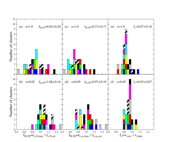
Figure 5: Distribution of $f_{H,{\rm 2D}}$ (left), $f_{H,{\rm 3D}}$ (middle), and $f_{v}$ (right) for all the simulated clusters (nine in total) at $z=0.05$ and $z=1.0$ viewed from three different line-of-sight directions. Different patterns of the histogram correspond to different clusters. The mean and 1$\sigma$ statistical errors are quoted in each panel.

Panels (a) to (d) in Figure 5 show the histograms of $f_{H,{\rm 2D}}$ and $f_{H,{\rm 3D}}$ for the nine clusters at $z=0.05$ and $z=1.0$. It is interesting to note that there is no significant systematic bias for $f_{H,{\rm 2D}}$ at $z=0$ even though the values of $r_{\rm c,X,fit}$ and $\beta_{\rm X,fit}$ are fairly different from $r_{\rm c,n_{e},fit}$ and $\beta_{\rm n_{e},fit}$. In fact, the mean values of $f_{H,{\rm 2D}}$ and $f_{H,{\rm 3D}}$ are close to unity well within the 1$\sigma$ statistical errors. As first discussed by Inagaki, Suginohara, & Suto (1995), any temperature structure could bias the value of $H_{0}$ estimated on the basis of equation (14). Although our simulated clusters do show some temperature structure, they do not seem to be strong enough to cause significant systematics. On the other hand, clusters at $z=1.0$ exhibit the systematic underestimate bias of $H_{0}$ by $\sim 20$%. This underestimate would result from the asphericity of the clusters because the values for the same clusters from three line–of–sight directions are significantly different.

4.2 Peculiar Velocity

The observed SZ flux $\Delta I_{\nu}$ is contributed from both the thermal and kinematic SZ effects (eqs.[2] and [7]). By using the different spectral dependence of these effects, we can estimate the peculiar velocity of the cluster (Sunyaev, Zel’dovich 1980; Rephaeli, Lahav 1991). Denote the total SZ flux in two bands, say $\nu=\nu_{1}$ and $\nu_{2}$, by

$$\Delta I_{j}=i_{0}[y~{}g(x_{j})-\tau(v_{r}/c)h(x_{j})],~{}(j=1~{}\mbox{and}~{}2),$$ (17)

where $x_{j}=h_{p}\nu_{j}/k_{\rm B}T_{\rm CMB}$. While the $y$-parameter is observable, $\tau$ is not unless the three-dimensional temperature profile is known independently. So one may estimate the peculiar velocity using the X-ray emission weighted temperature along the line–of–sight:

$$\langle T_{X}\rangle\equiv\frac{\displaystyle\int_{-\infty}^{\infty}T_{\rm e}(r)\alpha[T_{e}]n_{e}^{2}(r)dl}{\displaystyle\int_{-\infty}^{\infty}\alpha[T_{e}]n_{e}^{2}(r)dl},$$ (18)

as follows:

$$\frac{v_{r{\rm,est}}}{c}=\frac{k_{\rm B}\langle T_{X}\rangle}{m_{\rm e}c^{2}}\frac{g(x_{1})\Delta I_{2}-g(x_{2})\Delta I_{1}}{h(x_{1})\Delta I_{2}-h(x_{2})\Delta I_{1}}.$$ (19)

If clusters are isothermal, then $y=\tau(k_{\rm B}\langle T_{X}\rangle)/(m_{e}c^{2})$ and $v_{\rm r,est}$ is identical to $v_{r}$ in equation (17). For real clusters, however, the temperature profile is not strictly isothermal and estimates from equation (19) should be different from $v_{r}$ depending on the degree of non–isothermality. If we introduce a quantify the degree of non–isothermality of our simulated clusters:

$$f_{v}\equiv\frac{\tau}{y}\frac{k_{\rm B}\langle T_{X}\rangle}{m_{e}c^{2}},$$ (20)

then

$$v_{r,{\rm est}}=v_{r}\,f_{v}.$$ (21)

So $f_{v}$ can be regarded as a correction factor which relates $v_{r,{\rm est}}$ to the correct peculiar velocity:

We compute $f_{v}$ for all simulated clusters at $z=0.05$ and $z=1$ from three orthogonal line–of–sight directions (Figs. 5e and f). Compared with the histograms of $f_{H,{\rm 2D}}$ and $f_{H,{\rm 3D}}$, that of $f_{v}$ is more centrally concentrated. This is because $f_{v}$ is sensitive only to the non–isothermal structure along the line-of-sight while largely free from either the existence of local clumpiness or asphericity unlike $f_{H,{\rm 2D}}$ and $f_{H,{\rm 3D}}$. Since $\langle T_{X}\rangle$ has more weights on the high-density central regions, $f_{v}$ should be less than unity for clusters with central temperature drop as in our simulated ones. Panels (e) and (f) in Figure 5 indicates that this is the case. In summary, the estimates of $v_{r}$ are fairly reliable with overall fractional uncertainties $\sim 10$% at $z\approx 0$ and $\sim 20$% at $z=1$

5 Conclusions and Discussion

We have performed a series of numerical simulations with particular attention to the feasibility of estimating the Hubble constant $H_{0}$ and the cluster peculiar velocity $v_{r}$ via multi-band observations. Let us briefly summarize our conclusions here.

(i) A conventional isothermal $\beta$-model describes well our simulated clusters both in projected X-ray surface brightness and the SZ flux (Fig.1) as well as the three-dimensional gas density profile (Fig. 3). This is consistent with the analytical (Makino, Sasaki, Suto 1998) and numerical work (Eke, Navarro, Frenk 1998) on the basis of the universal density profile of dark matter halo (Navarro, Frenk, White 1997).

(ii) The best-fit values for the core radius and $\beta$-parameter change significantly depending on whether one attempts to fit the X-ray surface brightness, the SZ flux or the gas density (Fig.2). This reflects the non-isothermal temperature profile, local clumpiness and aspherical gas structure.

(iii) Provided that our simulated clusters constitute a representative sample of the observed clusters, the systematic and statistical errors in the estimates of $H_{0}$ and $v_{r}$ are relatively small (Fig.5); fractional uncertainties of the estimates of $H_{0}$ amount to $\sim 20$% mainly due to the departure from the isothermal and spherical gas density distribution. Those of $v_{r}$ range $\sim 10$% at $z\approx 0$ and $\sim 20$% at $z=1$. Since the three-dimensional temperature structure is very difficult to reconstruct from the projected temperature map (compare Figs. 3 and 4), the correction for the non-isothermality is not easy.

The similar temperature drop in the clusters discussed here was found earlier in simulations by Evrard (1990) and also reported in some observed clusters (e.g., Ikebe et al. 1997). Evrard (1990) ascribed this to the fact that earlier collapsed gas is only mildly shocked relative to the subsequent infalling gas. Although this is one reasonable interpretation, it could result simply from the shape of gravitational potential (Navarro, Frenk, White 1997; Makino, Sasaki, Suto 1998) or even from the lack of spatial resolution of simulations to represent the shock in the core regions. Therefore results from improved simulations are clearly needed; a larger number of gas and dark matter particles, $N=128^{3}$ and even $N=256^{3}$, is necessary to resolve the cluster core reliably. Then it makes sense to incorporate effects of cooling and heating which have been neglected here mainly because they are not so important with the mass resolutions of our present simulations. We have considered only one fairly specific cosmological model, and it is interesting to examine the cosmological model dependence of the results. Nevertheless we hope that our current results have highlighted several potentially important implications for the future cluster observations in the X–ray, mm, and submm bands.

We thank Tetsu Kitayama and Yi-Peng Jing for useful discussions and an anonymous referee for several constructive comments. We gratefully acknowledge the use of two publicly available numerical packages, Hydra by H.M.P.Couchman, P.A.Thomas and F.R.Pearce, and COSMICS by E.Bertschinger, for the present simulations. Numerical computations were carried out on VPP300/16R and VX/4R at the Astronomical Data Analysis Center of the National Astronomical Observatory, Japan, as well as at RESCEU (Research Center for the Early Universe, University of Tokyo) and KEK (National Laboratory for High Energy Physics, Japan). This research was supported in part by the Grants-in-Aid by the Ministry of Education, Science, Sports and Culture of Japan (07CE2002) to RESCEU, and by the Supercomputer Project (No.97-22) of High Energy Accelerator Research Organization (KEK).

REFERENCES

Barbosa, D., Bartlett, J.G., Blanchard, A., & Oukbir, J. 1996, A&A, 314, 13

Bertschinger, E. 1995, astro–ph/9506070.

Birkinshaw, M., Hughes, J.P. & Arnaud, K.A. 1991, ApJ, 379, 466

Couchman, H.M.P., Thomas, P.A. & Pearce, F.R., 1995, ApJ, 452, 797

Eke, V.R, Navarro, J.F., & Frenk, C.S. 1998, ApJ, submitted (astro–ph/9708070).

Evrard, A.E. 1990, ApJ, 363, 349

Hattori, M., Ikebe, Y., Asaoka, I., Takeshima, T., Böhringer, H., Mihara, T., Neumann, D.M., Schindler, S., Tsuru, T. & Tamura, T., 1997, Nature, 388, 146

Holzapfel, W.L., Ade, P.A.R., Church, S.E., Mauskopf, P.D., Rephaeli, Y., Wilbanks, T.M., & Lange, A.E. 1997, ApJ, 481, 35

Ikebe, Y., Makishima, K., Ezawa, H., Fukazawa, Y., Hirayama, Y., Honda, H., Ishisaki, Y.,Kikuchi, K., Kubo, H., Murakami, T., Ohashi, T., Takahashi, T., Yamashita, K. 1997, ApJ, 481, 660

Inagaki, Y., Suginohara, T.,& Suto, Y. 1995, PASJ, 47, 411

Kitayama, T., Sasaki,S., & Suto, Y. 1998, PASJ, in press (astro–ph/9708088).

Kitayama, T., & Suto, Y. 1996, ApJ, 469, 480

Kitayama, T., & Suto, Y. 1997, ApJ, 490, 557

Kobayashi, S., Sasaki,S., & Suto, Y. 1996, PASJ, 48, L107

Makino, N., Sasaki, S., & Suto, Y. 1998, ApJ, 497, April 20 issue, in press (astro-ph/9710344)

Masai, K. 1984, Ap&SS, 98, 367

Navarro, J.F., Frenk, C.S., & White, S.D.M. 1997, ApJ, 490, 493

Press, W. H., & Schechter, P. 1974, ApJ, 187, 425

Rephaeli, Y. & Lahav, O. 1991, ApJ, 372, 21

Rephaeli Y. 1995, ARA&A, 33, 541

Roettiger, K., Stone, J.M., & Mushotzky, R.F. 1997, ApJ, 482, 588

Rybicki, G.B., Lightman, A.P. 1979, Radiative Processes in Astrophysics ( Wiley: New York)

Schindler, S., Hattori, M., Neumann, D.M. & Böhringer, H., 1997, A& A, 317, 645

Silk, J. & White, S.D.M. 1978, ApJ, 226, L103

Silverberg, R.F., Cheng, E.S., Cottingham, D.A., Fixsen, D.J., Inman, C.A., Kowitt, M.S., Meyer, S.S., Page, L.A., Puchalla, J.L., & Rephaeli, Y. 1997, ApJ, 485, 22

Sunyaev R.A. & Zel’dovich Ya.B. 1972, Comments on Astrophys.& Space Phys., 4, 173

Sunyaev R.A. & Zel’dovich Ya.B. 1980, MNRAS, 190, 413

White, S. D. M., Efstathiou, G., & Frenk, C. S. 1993, MNRAS, 262, 1023

Figure 1: Projected profiles of X–ray surface brightness (top), the thermal SZ temperature decrement (middle), and the thermal SZ submm surface brightness (bottom) of clusters A and B at $z=0.05$ (left) and $z=1.0$ (right). The quoted error bars at each angular radius indicate the 1-$\sigma$ statistical dispersion computed from the 16 points on the projected circle with the radius.

Figure 2: The core radius (in physical lengths) and $\beta$-parameter for clusters A (triangles) and B (circles) at $z=0$ (open symbols) and $z=1$ (filled symbols). Different sizes of different symbols refer to the values from separate fits to $n_{e}(r)$, $S_{X}$ and $y$-parameter (from three orthogonal line-of-sight directions for the latter two).

Figure 3: Spherically averaged profiles of gas temperature (upper) and gas density (lower) of clusters A and B at $z=0.05$ (left) and $z=1.0$ (right). The radius $r$ is in physical lengths.

figure4a.jpg

figure4b.jpg

Figure 4: Projected views of clusters A (upper panels) and B (lower panels) at $z=1$ and $z\approx 0$. A box of (4Mpc)³ (in physical lengths) located at the center of each cluster is extracted. The X-ray emission–weighted temperature ($T_{X}$), X-ray surface brightness ($S_{X}$), and the SZ surface brightness at mm and submm bands ($|\Delta I_{\rm mm}|$ and $\Delta I_{\rm submm}$) are plotted on the projected X-Y plane by integrating over the line-of-sight direction (Z). The X and Y coordinates are in the physical lengths at the corresponding redshift, and related to the angular coordinate $\theta$ from the cluster center as $\theta d_{A}(z)$. At $z\approx 0$, $d_{A}(z)$ can be replaced by the real distance to the cluster from the observer.