PREHEATING AFTER INFLATION

In inflationary cosmology, the particles constituting the Universe are created after inflation in the process of reheating due to the interaction with the oscillating inflaton field. We briefly review the basics of the slow reheating, and the stage of fast preheating, when the particles are created explosively in the regime of parametric resonance. The non-perturbative, out-of-equilibrium character of the parametric resonance changes many features of reheating. For these proceedings, we will highlight a few aspects of preheating: the structural dependence of the parametric resonance on the inflationary model, including $V(\phi)={m^{2}\over 2}\phi^{2}$, ${\lambda\over 4}\phi^{4}$, $1-\cos{\phi\over f}$; “rescattering” of created particles; and phase transitions after inflation.

1 Reheating after Inflation

In modern versions of inflationary cosmology there is no pre-inflationary hot stage, the Universe initially expands quasi-exponentially in a vacuum-like state without temperature. During inflation, all energy is contained in the inflaton field $\phi$ which is slowly rolling down to the minimum of its effective potential $V(\phi)$. When chaotic inflation ends at $\phi\sim M_{p}$, the inflaton field begins to oscillate near the minimum of $V(\phi)$ with a very large amplitude $\phi\simeq{1\over 10}M_{p}$. In this scenario all the particles constituting the Universe are created due to the interaction with the oscillating inflaton field. Gradually, the energy of inflaton oscillations is transferred into energy of the ultra-relativistic particles. Eventually created particles come to a state of thermal equilibrium at some temperature $T_{r}$, which is called the reheating temperature. The transitional stage between inflation and the standard Big Bang is called the period of reheating after inflation.

To describe creation of elementary particles from the inflaton oscillations, we shall consider the interaction terms in the fundamental Lagrangian. The inflaton field $\phi$ may decay into bosons $\chi$ and fermions $\psi$ due to the interaction terms $-{1\over 2}g^{2}\phi^{2}\chi^{2}$ and $-h\bar{\psi}\psi\phi$, or into its own Bose quanta $\delta\phi$ due to the self-interaction $\lambda\phi^{2}\delta\phi^{2}$, or due to the gravitational interaction; $\lambda$, $g$ and $h$ are small coupling constants. In the case of spontaneous symmetry breaking at a scale $\sigma$, the term $-{1\over 2}g^{2}\phi^{2}\chi^{2}$ gives rise to the three-legs term $-g^{2}\sigma\phi\chi^{2}$. We will assume for simplicity that the bare masses of the fields $\chi$ and $\psi$ are very small. The elementary theory of reheating is based on the perturbative theory with respect to the coupling constants $\!{}^{{\bf?}}$. Inflaton oscillations are interpreted as a superposition of a number of $\phi$-particles, inflatons, at rest. Each inflaton has an energy equal to the frequency of the background oscillations. The decay rate of inflatons (or the particle production rate) is given by perturbation theory. For simplicity, consider the interaction $-{1\over 2}g^{2}F(\phi)\chi^{2}$ between the classical inflaton field $\phi$ and the quantum Bose field $\chi$ with the eigenfunctions $\chi_{k}(t)\,e^{-i{{\bf k}}{{\bf x}}}$ with comoving momenta ${\bf k}$. The temporal part of the eigenfunction obeys the equation

$$\ddot{\chi}_{k}+3{{\dot{a}}\over a}\dot{\chi}_{k}+{\left({{k^{2}}\over a^{2}}+g^{2}F(\phi)\right)}\chi_{k}=0\ ,$$ (1)

with the vacuum-like initial condition $\chi_{k}\simeq{e^{-ikt}\over\sqrt{2k}}$ in the far past. The WKB solution of Eq. (1) is

$$a^{3/2}\chi_{k}(t)\equiv X_{k}(t)={\alpha_{k}(t)\over\sqrt{2\omega}}\ e^{-i\int^{t}\omega dt}+{\beta_{k}(t)\over\sqrt{2\omega}}\ e^{+i\int^{t}\omega dt}\ ,$$ (2)

where the time-dependent frequency is $\omega_{k}^{2}(t)={{k^{2}}\over a^{2}}+g^{2}\phi^{2}$ plus a small correction $\sim H^{2},\dot{H}$; initially $\beta_{k}(t)=0$. For $|\beta_{k}|\ll 1$, an iterative solution
$\beta_{k}\simeq{\textstyle{1\over 2}}\int\limits_{-\infty}^{t}dt^{\prime}\,{\dot{\omega}\over\omega^{2}}\,\exp{\bigl{(}-2i\int\limits_{-\infty}^{t^{\prime}}dt^{\prime\prime}\omega(t^{\prime\prime})\bigr{)}}\sim g^{2}$ gives the standard result of perturbation theory for the particle occupation number $n_{k}=|\beta_{k}|^{2}$. The integral can be evaluated by the stationary phase method. For the three-legs interaction $g^{2}\sigma\phi\chi^{2}$, the perturbative result can be interpreted as separate inflatons decaying independently of each other into pairs of $\chi$-particles. The resulting rates of the three-legs processes $\phi\to\chi\chi$ and $\phi\to\psi\psi$ plus gravitational decay are given by

$$\Gamma_{\phi\to\chi\chi}={g^{4}\sigma^{2}\over 8\pi m_{\phi}}\ ,\ \ \Gamma_{\phi\to\psi\psi}={h^{2}m_{\phi}\over 8\pi}\ ,\ \ \Gamma_{g}={m_{\phi}^{3}\over 8\pi M_{p}^{2}}\ .$$ (3)

For the four-legs interaction a pair of inflatons is decaying independently into a pair of $\chi$-particles, $(\phi\phi\to\chi\chi)$. However, the decay of massive inflatons in this case is different. The transfer of energy from inflatons to the created particles rapidly decreases with the expansion of the Universe as ${1\over a^{4}}{d\over dt}(a^{4}\epsilon_{\chi})\propto a^{-6}.$ Therefore, the complete decay of the massive inflaton field in the theory with no spontaneous symmetry breaking or with no interactions with fermions is impossible.

Reheating completes at the moment $t_{r}$ when the Hubble parameter $H={1\over 2t}$ becomes equal to $\Gamma_{tot}$. Assuming thermodynamic equilibrium sets in quickly at the temperature $T_{r}$, one can equalize the energy density of the universe and thermal energy of created ultrarelativistic particles at the moment $t_{r}$. This gives the reheating temperature

$$T_{r}\simeq 0.1\sqrt{\Gamma M_{p}}\ ,$$ (4)

which is ultimately determined by the total decay rate $\Gamma_{total}$. In order to get numerical estimates for $t_{r}$, $\Gamma_{tot}$ and $T_{r}$, one should know the frequency of the inflaton oscillations and the coupling constants. The coupling constants of interaction of the inflaton field with matter cannot be too large, otherwise the radiative corrections alter the shape of the inflaton potential (unless SUSY eliminates radiative corrections). The necessary condition for the decay of inflaton oscillations is that their frequency is greater than the effective masses of created particles. Parameters of the inflaton potential are restricted from the constraints on amplitude of the cosmological fluctuations. All together it allows us to put constraints on the perturbative reheating. The largest total decay rate is $\Gamma<10^{-20}M_{p}$. It takes at least $10^{14}$ oscillations to transfer the energy of inflaton oscillations into the created particles, i.e. this reheating is very slow. The bound on the slow reheating temperature is $T_{r}<10^{9}\,\mbox{GeV}\ .$ This is a very small temperature, at which neither the standard mechanisms of baryogenesis in the GUTs work, nor cosmologically interesting heavy strings, monopoles and textures can be produced. In the slow reheating scenario with the potential ${m^{2}\phi^{2}\over 2}$, the post-inflationary stage of inflaton oscillations with a scalar factor $a(t)\sim t^{2/3}$ lasts sufficiently long. It can enhance the gravitational instability of density fluctuations, which leads to the formation of the primordial black holes for some specific spectra of the initial density fluctuations.

2 The Stage of Preheating

In the elementary theory outlined above, we made significant oversimplifications, assuming that each inflaton decays independently. However, interacting with quantum particles, inflatons act not separately, but as the coherently oscillating homogeneous field $\phi(t)$, as follows from Eq. (1). The oscillating effective frequency $\omega(t)$ and very large amplitude of the background oscillations $\phi(t)$ can result in a broad parametric resonance of the “oscillator” amplitude $\chi_{k}$. The smallness of $g^{2}$ alone does not necessarily correspond to small occupation number $|\beta_{k}|$, which can grow exponentially. Then the energy is very rapidly transferred from the inflaton field to other bose fields. This process occurs far away from thermal equilibrium, and therefore it is called preheating $\!{}^{{\bf?},{\bf?},{\bf?}}$. Reheating never completes at the first stage of parametric resonance; eventually the resonance becomes narrow and inefficient. The inflaton field decay is completed and created particles are settled in thermal equilibrium during the subsequent, final stages of reheating. However, the elementary theory should be applied not to the original inflaton oscillations, but to the products of its decay, or to its residual oscillations. The short stage of explosive preheating in the broad resonance out-of-equilibrium regime may have long-lasting effects on the subsequent evolution of the universe (compare to other cosmological epochs where particles temporarily can be out-of-equilibrium). It may lead to specific nonthermal phase transitions in the early universe and to the production of topological defects $\!{}^{{\bf?}}$, it may make possible novel mechanisms of baryogenesis $\!{}^{{\bf?},{\bf?}}$, and it may change the final value of the reheating temperature $T_{r}$.

The non-perturbative character of the parametric resonance changes many features of the particle creation from inflatons. For these proceedings, I will highlight only several interesting aspects of preheating, which we have learned recently: the structural dependence of the parametric resonance on the theory of inflation $V(\phi)$; “rescattering” (mode mixing) effect for created particles; and phase transitions after inflation.

3 Structure of Resonance and Inflaton Potential $V(\phi)$.

The resonance depends on the form of the background oscillations, which are defined by $V(\phi)$. We consider several popular models of $V(\phi)$.

3.1 Resonance in ${m^{2}\over 2}\phi^{2}$ Inflation

For the quadratic inflaton potential we have the background inflaton oscillations $\phi(t)\approx\phi_{0}(t)\cdot\sin{\left(m_{\phi}t\right)}$, $\phi_{0}(t)={M_{p}\over\sqrt{3\pi}}\cdot{1\over m_{\phi}t}$. The scalar factor is $a(t)\approx a_{0}t^{2/3}$. The amplitude of oscillations is decreasing as the universe expands, $\phi_{0}(t)\sim{0.1M_{p}}{a^{-3/2}}$ Let us consider ${g^{2}\over 2}\phi^{2}\chi^{2}$ interaction. The equation for the fluctuations (1) with $F(\phi)=\phi^{2}$ in a new time variable $z=mt$ takes the form reminiscent of the Mathieu equation. The dimensionless coupling parameter $q={{g^{2}\Phi^{2}}\over{4m^{2}}}$ depends on time via $\Phi^{2}\propto a^{-3}$. Without the expansion of the universe, that equation is exactly the Mathieu equation. Since ${m\over M_{p}}\simeq 10^{-6}$, we can have $q\simeq 10^{10}g^{2}\gg 1$, so the parametric resonance is broad. The regular Mathieu resonance can be described by its stability/instability chart. The Mathieu equation admits exponentially unstable solutions $\chi_{k}\propto\exp(\mu_{k}z)$ within the set of resonance bands, corresponding to the parametric resonance. For given parameter $q$, there are separated stability and instability zones. For $q\gg 1$ the parametric resonance is broad, with the width of the leading resonance band $\simeq 0.1\sqrt{gm\Phi}$ and with the characteristic exponent $\mu_{k}$ ranging from zero to its maximum $0.28$. In this case the eigenfunctions $\chi_{k}(t)$ have the form of the WKB solution (1) for all $t$ except very short time around moments $t_{j}$, $j=1,2,3,...$, where the background oscillating field crosses zero, $\phi(t_{j})=0$.

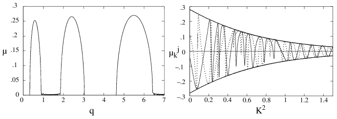
Figure 1: Left: characteristic exponent $\mu$ of the Mathieu equation as function of the parameter $q$ for the fluctuation with $k=0$. Right: the characteristic exponent $\mu^{j}_{k}$ in an expanding universe as function of $k$ for $j=5$ and $6$. $\mu^{j}_{k}$ changes dramatically with $j$ but within the theoretical envelope $\!{}^{{\bf?}}$.

Non-adiabatic changes of the amplitude $\chi_{k}(t)$ occur only in the vicinity of $t_{j}$, which can be described with the parabolic scattering. An essential parameter here is the phase $\theta_{k}=\int^{t_{j+1}}_{t_{j}}dt\sqrt{k^{2}+g^{2}\phi^{2}(t)}$ accumulating between two successive zeros of $\phi(t)$. If the parameter $q=const$, the phase $\theta_{k}$ as function of $k$ is not varying. Then we have a stable phase correlation/anticorrelation between successive scatterings at the parabolic potentials, which produces the sequence of stability/instability bands, see Fig. 1.

However, in an expanding universe the parameter $q$ is time-depended, $q={{g^{2}\Phi^{2}}\over 4m^{2}}$: $q\propto j^{-1}$. For the broad resonance case $q\gg 1$ this parameter can jump over a number of instability bands within a single oscillation, and the concept of stability/instability bands is inapplicable here. It is easy to understand that in this case the parametric resonance is a stochastic process. Indeed, for large initial values of $q$, the phase rotation between $t_{j}$ and $t_{j+1}$, $\delta\theta_{k}\simeq{{\sqrt{q}}\over 8j^{2}}$ is much larger than $\pi$ and therefore can be considered as a random number in the interval $[0,2\pi]$. As a result, there are no separate stability/instability bands, but each mode can be amplified or deamplified with every half period of the inflaton oscillation. An example of a stochastic $\mu_{k}$ is plotted in Fig. 1. Positive and negative occurrences of $\mu_{k}$ for $\kappa<\pi^{-1}$ appear in the proportion $3:1$, and the net effect is parametric amplification.

3.2 Resonance in ${1\over 4}\lambda\phi^{4}$ Inflation

For the theory with the potential $V(\phi)={1\over 4}\lambda\phi^{4}$ it is more convenient to express the background solutions via the conformal time $\tau=\int{dt\over a(t)}$ and conformal field $\varphi=a\phi$ variables: $\varphi(\tau)\approx\tilde{\varphi}~{}cn\left(\tau,{1\over\sqrt{2}}\right)$, $a(\tau)=\sqrt{2\pi\over 3}{\tilde{\varphi}\over M_{p}}\tau$, $\tilde{\varphi}$ is the amplitude of oscillations. The oscillations in this theory are not sinusoidal, but given by elliptic function. Let us consider a ${g^{2}\over 2}\phi^{2}\chi^{2}$ interaction of the inflaton. Eq. (1) for quantum fluctuations $\chi_{k}$ can be simplified in this theory. Using a conformal transformation of the mode function $X_{k}(t)=a(t)\chi_{k}(t)$, from Eq. (1) we obtain

$$X_{k}^{\prime\prime}+{\left(\kappa^{2}+{g^{2}\over\lambda}cn^{2}\Bigl{(}\tau,{1\over\sqrt{2}}\Bigr{)}\right)}X_{k}=0\ ,$$ (5)

where $\kappa^{2}={k^{2}\over\lambda\tilde{\varphi}^{2}}$, and $q={g^{2}\over\lambda}$. The equation for fluctuations does not depend on the expansion of the universe and is completely reduced to the similar problem in Minkowski space-time. This is a special feature of the conformal theory ${1\over 4}\lambda\phi^{4}+{1\over 2}g^{2}\phi^{2}\chi^{2}$. The mode equation (5) belongs to the class of Lamé equations $\!{}^{{\bf?},{\bf?},{\bf?}}$ The combination of parameters $q=g^{2}/\lambda$ ultimately defines the structure of the parametric resonance in this theory. This means that the condition of a broad parametric resonance does not require a large initial amplitude of the inflaton field, as for the quadratic potential. The strength of the resonance depends non-monotonically on this parameter. The stability/instability chart of the Lamé equation (5) in the variables $\left(\kappa^{2},{{g^{2}}\over\lambda}\right)$ was constructed in $\!{}^{{\bf?}}$ (see also P.Greene’s contribution to this volume). On the left panel of Fig. 2 we show slices of the Lamé stability/instability chart as a functions $\mu_{k}$ for several values of parameter $g^{2}/\lambda$.

To see how the general theory of the Lamé resonance works, for illustration let us consider parametric resonance in the model of the self-interacting two-component scalar field $(\phi_{1},\phi_{2})$ with the effective potential $V(\phi)={\lambda\over 4}(\phi_{1}^{2}+\phi_{2}^{2})^{2}$. For the two component inflaton scalar field, we always can align the classical background field with one of the components, say $\phi_{1}(t)$. The equations for the quantum fluctuations for two components $\delta\phi_{1}$ and $\delta\phi_{2}$ are different. The equation for the mode function of fluctuations in the direction $\phi_{1}$ is

$$\ddot{\phi_{1k}}+3{{\dot{a}}\over a}~{}{\dot{\phi}_{1k}}+{\left({k^{2}\over a^{2}}+3\lambda\phi_{1}^{2}\right)}\phi_{1k}=0\ .$$ (6)

The equation for the mode function of fluctuations in the direction $\phi_{2}$ is

$$\ddot{\phi_{2k}}+3{{\dot{a}}\over a}~{}{\dot{\phi}_{2k}}+{\left({k^{2}\over a^{2}}+\lambda\phi_{1}^{2}\right)}\phi_{2k}=0\ .$$ (7)

In some early papers on preheating the iteration series in the small parameter $\lambda$ was used. This approach is incorrect. Indeed, using the conformal transformation of the mode functions $\varphi_{1k}(t)=a(t)\phi_{1k}(t)$ and $\varphi_{2k}(t)=a(t)\phi_{2k}(t)$, we can reduce the equations (6), (7) to the general equation (5) with particular value of the parameter $q=3$ and $1$ respectively, so there is no small parameter associated with the resonance. In both cases $q=1,3$ there is only one instability band, but the strength of the resonance is different $\!{}^{{\bf?},{\bf?},{\bf?}}$. The resonance in the “inflaton” direction $\phi_{1}$ is weak, maximal value of the characteristic exponent of the fluctuations $\phi_{1k}\propto e^{\mu_{1}\tau}$ is $\mu_{1}\approx 0.036$; the resonance in the other direction $\phi_{2}$ is much stronger and broader, $\mu_{2}\approx 0.147$, see Fig. 2.

3.3 Resonance in Sine-Gordon theory

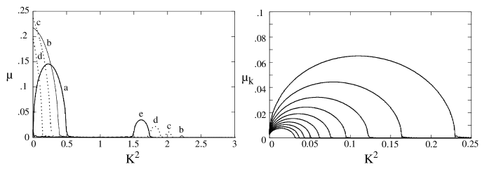
Figure 2: Left: The characteristic exponent $\mu_{k}$ for the Lamé equation (5) as a function of $k^{2}$ (in units of $\lambda\tilde{\varphi}^{2}$ ) for ${g^{2}\over\lambda}=1.0,1.5,2.0,2.5$ and $3.0$, labeled $a$ through $e$ respectively. Right: $\mu_{k}$ as a function of $k^{2}$ (in units of $m^{2}$) in the Sine-Gordon theory. Different curves correspond to different values of the background misalignment angle, $\theta_{0}$, from the outer curve inwards $\theta_{0}=1.67,1.25,1.0,0.83,0.71,$ $0.625,0.56,0.5,0.45,0.42,0.38,0.36.$

The Sine-Gordon potential $V(\phi)=m^{2}f^{2}\left(1-\cos{\phi\over f}\right)$ is the prototype of the natural inflation scenario, as well as the cosmic axions. Let us consider small quantum fluctuations $\delta\phi$ around oscillating homogeneous background field $\phi(t)$, which can be excited due to the self-interaction. At the moment we neglect the expansion of the universe. The equation for the temporal part of the eigenfunctions of fluctuations $\phi_{k}(t)$ is

$$\ddot{\phi_{k}}+{\left(k^{2}+m_{a}^{2}\,\cos{\phi\over f}\right)}\phi_{k}=0\ .$$ (8)

Since the background oscillations are periodic, there is parametric amplification of the fluctuations $\phi_{k}(t)$. We $\!{}^{{\bf?}}$ have derived the general analytic solution of this equation for an arbitrary initial amplitude $\phi_{0}$, or for an arbitrary misalignment angle $\theta={\phi_{0}\over f}$. The characteristic exponent $\mu_{k}$ as function of $k$ is plotted in Fig (2). There is always only a single resonance band. The value of $\mu_{k}$ strongly depends on the phase $\theta_{0}$. In the important case of small misalignment angle ${\theta_{0}}\ll 1$, the general formula for $\mu_{k}$ is reduced to the simple expression $\mu_{k}={k\over 4m_{a}}\sqrt{{\theta_{0}^{2}}-{4k^{2}\over m_{a}^{2}}}$. In this case the maximum value $\mu_{k}={\theta_{0}^{2}\over 16}$ at ${k^{2}\over m_{a}^{2}}={\theta_{0}^{2}\over 8}$. The resonance band in this limit is $0\leq{k^{2}\over m_{a}^{2}}\leq{\theta_{0}^{2}\over 4}$. It is instructive to return to the equation for fluctuations (8), and perform there a small $\theta$ approximation to the $\cos\theta$ term. This gives us the Mathieu equation with the parameter $q={\theta_{0}^{2}\over 8}$. We would predict a set of resonant bands, the first resonance band being located at ${\theta_{0}^{2}\over 8}\leq{k^{2}\over m_{a}^{2}}\leq{3\theta_{0}^{2}\over 8}$, which is shifted from the actual instability zone. The difference between the actual Sine-Gordon resonance and its Mathieu approximation is even more noticeable if we include the expansion of the universe. The parametric resonance due to the self-interaction is not effective both for the natural inflation and for axions, because the amplitude is quickly $\theta_{0}\sim a^{-3/2}$ decreasing with the expansion, but not because of the redshift from the resonance as was thought previously. Certainly, if we allow coupling to other bosons, say a $g^{2}\phi^{2}\chi^{2}$-interaction, then preheating in natural inflation can be very efficient.

4 “Rescattering” of created particles

So far we have treated the fluctuations $\chi$ of $\delta\phi$ as test fields in a given background $\phi(t)$ and $a(t)$. Due to the exponential instability of fluctuations, one expects their backreaction on the background dynamics is gradually accumulating until it changes the resonance itself. There are two especially important effects of backreaction. First, fluctuations may change the frequency of background oscillations, which can be taken into account in the Hartree approximation $\!{}^{{\bf?},{\bf?}}$. The second effect is the production of the inflaton fluctuations, which occurs due to the interaction of created particles $\chi$ (or $\delta\phi$) with the inflatons at rest. One can visualize this process as scattering of $\chi$ particles on the oscillating field $\phi(t)$, taking inflatons away from the homogeneous oscillating condensate. Fluctuations of Bose fields generated with large occupation number can be considered as classical waves with gaussian statistics. Therefore, all the field $\phi(t)$, $\chi$, $\delta\phi$ can be treated as interacting classical waves. This opens an avenue to study preheating through lattice numerical simulations $\!{}^{{\bf?},{\bf?}}$.

The theory of “rescattering” can be illustrated with the two-component self-interacting model $V(\phi)={\lambda\over 4}(\phi_{1}^{2}+\phi_{2}^{2})^{2}$, where the inflaton field is identified with the first component $\phi_{1}$. In this model we have the cross-interaction term $\lambda\phi_{1}^{2}\phi_{2}^{2}$. The rescattering of the $\phi_{2}$ particles on the classical field $\phi_{1}$ leads to the production of $\phi_{1}$ particles in the process $\phi_{2,\vec{k}}~{}\phi_{1}\to\phi_{2,\vec{k}^{\prime}}~{}\phi_{1,\vec{k}-\vec{k}^{\prime}}$. The generation of fluctuations $\phi_{1}$ due to this process can be incorporated in the mode equation (7) with the scattering term $\lambda\phi_{1}(\tau)\int d^{3}k^{\prime}\phi_{2,\vec{k}-\vec{k}^{\prime}}\phi_{2,\vec{k}^{\prime}}$. In conformal variables, the fluctuations $\varphi_{1k}$ due to the rescattering are given by the formula (cf. $\!{}^{{\bf?},{\bf?}}$):

$$\varphi_{1,k}(\tau)=-{1\over{(2\pi)^{2}\omega_{k}}}\int_{0}^{\tau}d\tau^{\prime}\sin\omega_{k}(\tau-\tau^{\prime})\phi_{1}(\tau^{\prime})d^{3}k^{\prime}\varphi_{2,\vec{k}-\vec{k}^{\prime}}(\tau^{\prime})\varphi_{2,\vec{k}^{\prime}}(\tau^{\prime})\ ,$$ (9)

where $\omega_{k}$ is the effective frequency of Eq. (5). From this it follows that the amplitude $\varphi_{1,k}(\tau)$ grows with time as $e^{2\mu_{2}\tau}$, where $\mu_{2}=0.147$. Therefore ${\langle\varphi_{1}^{2}\rangle}$ evolves in time even faster than ${\langle\varphi_{2}^{2}\rangle}$. Analysis of Eq. (9) shows that the process $\delta\phi_{2,\vec{k}}~{}\phi_{1}\to\delta\phi_{2,\vec{k}^{\prime}}~{}\delta\phi_{1,\vec{k}-\vec{k}^{\prime}}$, strictly speaking, does not correspond to the “particle-like” rescattering, but rather to the interaction of waves, mode mixing.

5 Phase Transitions from Preheating

The theory of cosmological phase transitions is one of the main topics in modern cosmology. Cosmological phase transitions in GUTs, which may happen at $T_{c}\sim 10^{15}-10^{16}$ GeV, could give rise to primordial monopoles and other topological defects, which could either kill popular cosmological models, or help them. The possibility of the phase transitions from preheating is based on the following idea $\!{}^{{\bf?}}$. The number of particles created during preheating can be very large. These particles initially are far away from thermal equilibrium. They may change the shape of the effective potential, which may lead to specific nonthermal phase transitions soon after inflation. Nonthermal phase transitions induced by preheating are similar to the usual high-temperature phase transitions, but they may occur even in the models where the high temperature effects cannot lead to symmetry restoration. This is because fluctuation amplitudes $\langle\phi^{2}\rangle$ from resonant amplification can be very large.

As an example, let us consider a two-component scalar field $(\phi_{1},\phi_{2})$ with the effective potential

$$V(\phi)={\lambda\over 4}(\phi_{1}^{2}+\phi_{2}^{2}-{\rm v}^{2})^{2}\ .$$ (10)

If we identify the $\phi_{1}$ component with the “inflaton” direction (as in section 3.2), the effective mass of the background field is $m_{eff}^{2}=-{\rm v}^{2}+3\lambda\phi_{1}^{2}+3\lambda\langle\delta\phi_{1}^{2}\rangle+\lambda\langle\delta\phi_{2}^{2}\rangle$. We shall consider the growth of fluctuations in this model. At the beginning one can neglect the tachyonic term. Then we can use the results of Sec. 3.2, $\langle\delta\phi_{1}^{2}\rangle\propto e^{2\mu_{1}\tau}$, $\langle\delta\phi_{2}^{2}\rangle\propto e^{2\mu_{2}\tau}$, $\mu_{2}\gg\mu_{1}$. However, the mode mixing due to the cross-interaction leads to the faster growth of fluctuations $\langle\delta\phi_{1}^{2}\rangle\propto e^{4\mu_{2}\tau}$. If ${\rm v}^{2}>10^{-4}\tilde{\varphi}^{2}$, the generation of fluctuations will be completed before the bifurcation in the evolution of the the background field occurs at $\phi_{1}\simeq{\rm v}$. By that moment, we will have the amplitude of fluctuations comparable to that of the background field, $\langle\delta\phi_{1}^{2}\rangle\sim\langle\delta\phi_{2}^{2}\rangle\sim\phi_{1}^{2}$. In this model we have symmetry restoration alongside with the residua oscillation of the background component $\phi_{1}(t)$, and what is most important, the formation of strings. Notice that the string formation mechanism is somewhat different from the Kibble mechanism. Lattice simulations of the self-consistent non-linear dynamics clearly demonstrate the formation of topological defects in the model $\!{}^{{\bf?}}$.

References

References

- [1] P.Greene, L. Kofman, A. Linde & A. Starobinsky, Phys. Rev. D 56, 6175 (1997).
- [2] P.Greene, L. Kofman, & A. Starobinsky, in preparation
- [3] D. Boyanovsky, H.J. de Vega, R. Holman, D.S. Lee, & A. Singh, Phys. Rev. D 51, 4419 (1995).
- [4] D. Boyanovsky, H.J. de Vega, R. Holman, & J.F.J. Salgado, Phys. Rev. D 54, 7570 (1996).
- [5] D. Kaiser Phys. Rev. D 56, 706 (1997).
- [6] S. Khlebnikov & I. Tkachev, Phys. Rev. Lett. 77, 219 (1996); Phys. Lett. B 390, 80 (1997); Phys. Rev. Lett. 79, 1607 (1997)
- [7] L. Kofman, A. Linde, & A. Starobinsky, Phys. Rev. Lett. 73, 3195 (1994).
- [8] L. Kofman, A. Linde, & A. Starobinsky, Phys. Rev. Lett. 76, 1011 (1996); I. Tkachev, Phys. Rev. Lett. 76, 35 (1996).
- [9] L. Kofman, A. Linde, & A. Starobinsky, Phys. Rev. D 56, 3258 (1997).
- [10] E. Kolb, A. Linde, & A. Riotto, Phys. Rev. Lett. 77, 4960 (1996).
- [11] A. Linde, Particle Physics and Inflationary Cosmology (Harwood 1990).
- [12] I. Tkachev, L. Kofman, A. Linde, A. Starobinsky & S. Khlebnikov, in preparation.
- [13] T. Prokopec & T.G. Roos, Phys. Rev. D 55, 3768 (1997).
- [14] Y. Shtanov, J. Traschen, & R. Brandenberger, Phys. Rev. D 51, 5438 (1995).